Panel Attrition

Abstract

Attrition is the process of dropout from a panel study. Earlier studies into the determinants of attrition study respondents still in the survey and those who attrited at any given wave of data collection. In many panel surveys, the process of attrition is more subtle than being either in or out of the study. Respondents often miss out on one or more waves, but might return after that. They start off responding infrequently, but more often later in the course of the study. Using current analytical models, it is difficult to incorporate such response patterns in analyses of attrition. This article shows how to study attrition in a latent class framework. This allows the separation of different groups of respondents, that each follow a different and distinct process of attrition. Classifying attriting respondents enables us to formally test substantive theories of attrition and its effects on data accuracy more effectively.

Keywords

panel surveys attrition latent class analysis nonresponse error LISS

Attrition or permanent dropout from a panel study is one of the most important sources of nonsampling error in panel surveys. Even modest attrition rates can greatly reduce the number of respondents over the course of the panel, reducing statistical power. More importantly, when attrition is selective, attrition can lead to biased survey estimates. Although the process of attrition is in many ways similar to nonresponse in a cross-sectional survey, there is one important difference. All respondents who drop out in a panel survey did at least participate in one wave of the study. Although panel survey managers aim to interview everyone at every wave, many respondents participate infrequently, or drop out altogether. This article aims to show how different theoretical causes for attrition in a panel survey can be tested empirically and lead to a typology of attrition processes.

The process of attrition will differ across respondents. While some respondents always loyally participate, others participate infrequently, or drop out all of a sudden. At every request to participate in a wave of the survey, respondents have a certain propensity to participate that ranges from 0 (certain not to participate) to 1 (certain to participate). The size of the propensities will depend on the history of response behavior in the panel survey. Respondents who always participate have a higher propensity to participate when a request for participation is sent than those who have not responded in earlier waves.

The survey methodology literature has described a number of general causes for the fact that response propensities vary across both individuals and time. Commitment to the survey, habit, and incentives can positively affect response propensities and lead to continued participation, while panel fatigue and shocks affect the propensities negatively (Laurie, Smith, and Scott 1999; Lemay 2010). We can distinguish four distinct mechanisms that can lead to declining response propensities and attrition.

The first reason for attrition is “absence of commitment” (Laurie, Smith, and Scott 1999). Some respondents really never wanted to participate at all in the panel study but were convinced to participate in the first wave. If participation itself does not change their commitment to the panel survey quickly, these respondents are very likely to drop out in wave 2 or wave 3. Conversely, when commitment is high, respondents attach value to their participation in the panel. This will result in a group of respondents who are very loyal and lead to continued participation in (almost) all waves.

Repeated participation in a panel survey may lead to “habit,” even in the absence of high commitment. When survey participation becomes a habit, respondents do no longer consciously think about responding, but participate, because they have done so all along. Once this habit is broken, the respondent is subsequently at a higher risk of missing more waves, or attriting altogether (Davidov et al. 2007). Seeing panel participation as a habit explains why wave nonresponse in panel surveys is generally seen as an indicator for possible attrition at a later moment.

The third reason for attrition is panel fatigue. After a prolonged period of participation, many respondents may feel like they have done their duty. The subjective burden that panel participation causes weighs heavier with every wave. This leads to slowly declining response propensities until respondents drop out. The point where the burden becomes too heavy is likely to be different for every respondent (Lemay 2010; Lipps 2009).

The fourth reason for panel attrition is “shock” (Lemay 2010). A shock may lead to sudden dropout from a panel. Shocks can be caused by life-changing events like a serious illness (or death), moving, or changes in the composition of the household. A shock may also be caused by one particular unpleasant experience as a panel member, like a badly designed questionnaire, the wrong use of personal data, or disturbing survey topics.

We never have direct information on the factors that affect response propensities for both respondents and nonrespondents. Instead, attrition studies use data collected for all respondents at earlier waves, and classify respondents based on covariates that are closely related to the propensity to participate.

While analyzing the determinants or consequences of attrition, some authors pool all wave-on-wave attrition patterns (Nicoletti and Peracchi 2005; Watson and Wooden 2009), and simply discern two groups: the attriters and stayers. This approach ignores the possibility that attrition for waves 2 to 3 is different than attrition for waves 7 to 8; it does not allow response propensities to change with time. Another approach is to study nonresponse separately for every wave-on-wave transition (Uhrig 2008). Apart from the fact that this yields many analyses, it is hard to deal with respondents returning to the survey, which implies that respondents can attrite multiple times. Other authors have only focused on the final state of attrition and have limited themselves to predict whether attrition occurs or not (Tortora 2009), or use duration models controlling for wave effects (Lipps 2009). Durrant and Goldstein (2010) take a more integrative approach and look at all possible monotone attrition patterns in a four-wave panel study. With nonmonotone attrition, and longer panel spans, this approach is also challenging. Finally, Voorpostel (2009) and Behr, Bellgardt, and Rendtel (2005) follow the example of Fitzgerald, Gottschalk, and Moffitt (1998) and separate a group of attriting (“lost”) from returning (“ever out”) respondents, thereby also allowing for nonmonotone attrition. As the panel study matures, one should however distinguish between more and more differing groups of “ever-out” respondents.

In the data that we use in this study, respondents complete questionnaires monthly. The high frequency of data collection implies that wave nonresponse is even more likely to occur at any given wave than in other panel surveys and that nonmonotone attrition occurs often. The approach that we take to model attrition is different from earlier attrition studies as we model attrition in a latent class framework. The underlying factors that affect survey participation can be summarized in a response propensity that allows us to distinguish several classes of respondents who each follow a different attrition process. This approach allows the response propensities to vary across individuals and across time for different groups of attriters, enabling us to study who attrites, when they attrite, and how the attrition process takes place. The classification involves modeling the response process with mixture models that combine categorical and continuous latent variables. The use of latent class models to study attrition has earlier been attempted by Lemay (2010), but was unsuccessful; probably due the combination of high computational demands, and the fact that ineligibility, noncontact, and refusals were separately modeled.

After we discern different classes of attriters, we conclude this article by showing how attrition classes affect attrition bias, and discuss how latent variable models can be successfully used to study and prevent attrition.

Who Attrites?

Most of our knowledge about the correlates of attrition stems from panel studies in which respondents are interviewed by trained interviewers. In such situations, it is useful to make a distinction in attrition due to failure to locate the sample members, noncontacts, and refusals (Lepkowski and Couper 2002). In this study, we use data from an Internet panel that contacts respondents by e-mail. Respondents whose invitations to the survey bounced were called to update their e-mail address. Therefore, it is hard to distinguish between attrition due to nonlocation, noncontacts, and refusals. We therefore only discuss how the respondents’ background characteristics lead to different attrition processes within our sample. Often, there is no clear link between sociodemographic variables and attrition theories. They can however be important for bias assessment and correction.

Women have been shown to attrite less often than males (Behr, Bellgardt, and Rendtel 2005; Lepkowski and Couper 2002). Women are thought to be more conscientious and more committed and thus miss fewer waves, although evidence for this is mixed (Uhrig 2008). People with a higher socioeconomic status—higher education and income—attrite less, although effects are usually small (Watson and Wooden 2009). People from ethnic minorities attrite more often (Lipps 2009). The reasons for this might be panel-specific, but we can speculate that they might perceive a higher burden due to language or cultural differences.

Other determinants of attrition are marital status (being not married), whether someone moved (or is planning to move) (Lillard and Panis 1998) and the size of the household (Lipps 2009). The fact that household size is important is probably due to higher contact propensities and/or persuasion of other household members to either stay involved in the panel survey or also dropout. Age has been found not to be related to attrition, although the oldest old and children around the age of 18 are more at risk (Lipps 2009). Most of the effects of sociodemographic variables are either related to contactability (and thus do only weakly apply to an Internet panel) or seem to disappear when controlling for a change in household situation (the young), or health (the oldest old; Jones, Koolman, and Rice 2006).

Sociopsychological variables are deemed to have more explanatory power than demographic variables in explaining attrition and can be closely linked with attrition theories. Respondents with specific personality traits are more likely to drop out because of panel fatigue or become committed to a survey. People with high levels of agreeableness-part of the Big Five personality scale (Costa, Paul, and McCrae 1992) are more cooperative, while conscientious people are said to be reliable, determined, and have a strong need for achievement (Costa, Paul, and McCrae 1992), which should all lead to higher commitment. On the other hand, people who score high on the scale extraversion are reported to become easily bored or distracted, possibly leading to panel fatigue, dropout, or infrequent response behavior (Costa, Paul, and McCrae 1992). It is not clear how neuroticism and openness to experience, the other Big Five personality factors, affect survey participation.

Other personality characteristics that have been linked to increased survey participation are whether people like to do cognitive tasks and evaluate. High levels of “need for cognition” (Tuten and Bosnjak 2001), and “need to evaluate” (Bizer et al. 2004), should also lead to commitment to the panel survey, and prolonged survey participation.

Panel commitment and fatigue can also be measured more directly by asking respondents’ attitude toward the panel survey (Rogelberg et al. 2001; Stocké 2006). Whether a respondent attributes “value” to his or her own answers or “enjoys” it indicate that commitment is present. Asking respondent directly about the burden they perceive while completing the survey can serve as an indicator of panel fatigue (Hill and Willis 2001), although social desirability can be a potential problem in asking the respondent directly about his survey experience.

Even when panel respondents are committed and have a habit of participating, a “shock” due to death, moving, or a negative survey experience may lead to sudden attrition. In order to predict panel shocks, one would need detailed information on covariates in every wave; so-called time-variant covariates. Practical considerations often lead panel managers to only ask about a small set of characteristics in every wave. Most often, these are related to the household composition and a few other “core” variables, as change in address and employment situation (Uhrig 2008). One variable that is often linked to attrition, especially for older respondents, is health status at every wave (Watson and Wooden 2009), which might fluctuate with every wave. Survey methodologists have in recent years been exploring the use of paradata for explaining attrition. Similar to the respondents’ attitude toward surveys, paradata can signal commitment or panel fatigue. Loosveldt, Pickery, and Billiet (2002) showed, for example, that the number of item missings is indicative of attrition in later waves. Hill and Willis (2001) furthermore hypothesize that in self-administered surveys, long interviewing time is negatively associated with future participation. Although we have recorded data on all these aspects, we focus in this article on structural or time-invariant determinants of attrition, as the inclusion of time-variant covariates further increases the high computational demands of the models we present. We will show how we can still evaluate the shock hypothesis indirectly, by studying whether response propensities in the different classes show dramatic shifts at any given time.

Method

Data

The data for our study stem from the Longitudinal Internet Studies for the Social Sciences (LISS).¹ This panel was started in autumn of 2007, and interviews respondents monthly on a wide range of topics. The original sample for the panel was a simple random sample of Dutch households, who were contacted and recruited using a mixed-mode design. After initial contact, all household members were asked to participate in the panel survey. The participation rate in wave 1 amounted to 49 percent (American Association for Public Opinion Research 2009). Those households that did not have a computer with broadband Internet connection prior to participation were provided with one (from here on called SimPC) by LISS. People who received a SimPC were likely to be over 65, be living with a partner, and have lower incomes than the average sample member. Inclusion of people without Internet into the LISS sample members however successfully reduced nonresponse bias (Leenheer and Scherpenzeel 2011).

For now, we only use data from the first 48 full waves of the LISS panel, spanning the period of January 2008 to December 2011. About 20 percent of respondents started some months before January 2008, as the panel was built gradually. We discarded those interviews, but chose to keep the data from those respondents after January 2008. Likewise, we chose to not include the data recorded in the recruitment interview because of missing data and potential mode effects. January 2008 was therefore set as the first wave of Internet interviewing for all respondents.² This resulted in binary response data for 48 waves and 8,148 cases. Survey break offs were included as a wave response (1), and amounted to 2 percent of all responses. Interviewing time is about half an hour per month, and respondents receive a reward of about €15 for every hour of completing questionnaires. They are reminded in case of initial nonresponse in a specific wave, and occasionally receive information about research findings. Despite this, most panel respondents in the LISS panel fail to complete one or more of the monthly surveys, before reentering the survey at a later time. This amounts to a total of 4,973 different missing data patterns.

Instruments

We use a variety of covariates from the LISS that were mostly measured in one of the initial waves of the study. Over the course of the panel, respondents in the LISS panel were sometimes allowed to “catch up” on questionnaires they missed at a later wave of the survey. We coded such behavior as a wave nonresponse for the wave in which the questionnaire was originally fielded, but did include data on any of the covariates.

First, we use a set of sociodemographic characteristics that we treat as time-invariant: gender, age, net income (13 categories), highest education (7 categories), urbanicity, living with a partner, and having a SimPC. As psychological factors, we used the Big Five questionnaire (Goldberg et al. 2006) to construct five-factor scores (Openness, Conscientiousness, Extraversion, Agreeableness, and Neuroticism). Another factor score “need to evaluate” was computed using a questionnaire by Jarvis and Patty (1996), while a factor score for “need for cognition” was computed using the same procedure (Cacioppo and Petty 1983). All factor scores were computed using maximum likelihood extraction, and oblique rotation in the case of personality. Bartlett factor scores were saved (Tabachnick and Fidell 2007) and further used in our analyses. Other important determinants of panel attrition are the respondents’ attitude toward the survey. The LISS panel contained nine questions about one’s general attitude toward surveys. They ask the respondents whether they enjoy (1) Internet surveys and (2) being interviewed, whether surveys are (3) interesting and (4) important for society, whether (5) things can be learned, whether (6) completing surveys is a waste of time, (7) the perceived burden of survey requests (8) whether surveys invade privacy, and (9) whether answering questions is exhaustive. A study by de Leeuw et al. (2010) has suggested that the nine items load on three factors: survey enjoyment, survey value, and survey burden, but we have included all nine questions separately to assess in detail how these evaluation criteria determine panel participation.

Model

We modeled the response data using a latent class framework. The advantage of using latent classes is that respondents are categorized based on the similarity of their response patterns. We treat a wave response in a particular wave as 1 and nonresponse as 0. There are three general approaches to specify the latent classes, that all differ in the way they treat the longitudinal nature of the data and handle unobserved heterogeneity: (1) latent class analysis (LCA), (2) latent class growth analysis (LCGA), and (3) growth mixture models (GMM). In LCA, all wave responses are being treated as independent from each other; that is, the longitudinal nature of the data is ignored. Classes are formed on similar response patterns, but the response patterns in any class can take any form. LCGA explains the response patterns parametrically. Here, all wave responses are explained by a latent intercept (i), linear slope (s), and/or quadratic slope parameter (q). This means that response patterns within every class follow a distinct pattern of growth (or here decline) in response propensities over the course of the panel study and that this pattern is the same for everyone in this group.

The LCGA model is less flexible than the LCA model, but this is offset by the fact that fewer estimated parameters can lead to a better relative model fit (Kreuter and Muthén 2008). An extension of the LCGA model forms the GMM. The GMM incorporates intraclass variability in the variances of the intercepts, slopes, and/or the quadratic terms.³ This allows for unobserved heterogeneity within every class (Feldman, Masyn, and Conger 2009), which means that respondents are allowed to have a higher or lower intercept, slope, and/or quadratic slope than other respondents in their class. To increase the quality of the classifications into classes, the different latent classes in all models are regressed on the set of covariates. The covariates were not regressed on the variance components of the intercept and slopes of the GMM, as it is not our goal to explain the variance terms of the growth parameters in the GMMs.

As it was unclear which of the three families of latent class models would explain attrition best, and how many attrition classes are necessary, we ran a set of models, each with a different number of classes, and select the model that performs best. We used five evaluation criteria for this. The Bayesian Information Criterion (BIC) serves as our primary heuristic for model comparison. This statistic is similar to absolute fit indices (e.g., Akaike’s Information Criterion and Consistent Akaike’s Information Criterion), but it assigns a greater penalty to model complexity, and hence has a greater tendency to prefer the more parsimonious model (Nylund, Asparouhov, and Muthén 2007). Lower values for BIC indicate a better relative fit of the model to our data. As absolute differences for BIC between competing models can be small, it is desirable to use Lo–Mendell–Rubin Test (LMRT) or bootstrapped likelihood ratio test (BLRT) to specifically test whether one model fits significantly worse than the same model with one latent class less (Nylund, Asparouhov, and Muthén 2007). Apart from the values of BIC and the LMRT and BLRT, we chose to also rely on values of the entropy (Celeux and Soromenho 1996) as a criterion for the classification quality, and the substantive results of the best-performing models. For this, we primarily looked at observed attrition patterns of every class after estimating the model and the size of the smallest class (Muthén 2006).

All models were estimated using MPLUS 7.11 (Muthén and Muthén 2013). Because of the fact that individuals are clustered within households, we correct the standard errors using the robust maximum likelihood estimator (Muthén and Muthén 2010). Any missing data that we have on the covariates in our model were multiply imputed using the saturated model within the Bayesian module of Mplus (Muthén 2010).⁴ We initially ran all models using five imputed data sets, and repeated our analyses with 20 imputed data sets for the final model, to make sure our results were robust.⁵

Results

Table 1 shows the fit of a range of tested models, each with 1 to 15 classes. In every model, we see that the BIC values generally decrease when we add more classes, indicating that there are indeed several subgroups in the LISS panel with a distinctive attrition pattern. When consecutively estimating the models with more classes, the BIC values reach a minimum, after which they either start increasing again. At this point, the estimation often fails to converge. Nonconvergence is typical for overspecified mixture models, indicating that a more parsimonious model should be preferred (Nylund, Asparouhov, and Muthén 2007). The best models in terms of their BIC values are shown in boldface. The latent class models perform best of the three families of models. This implies that attrition in the LISS panel does not take a parametric linear form, as the LCGA and GMMs assume, but follows a nonparametric trend.

Table 1.

BIC Values for Different Sets of Latent Variable Mixture Models Explaining Attrition Patterns.

BIC Values for Model/Classes			GMM
Variance for Growth Parameters	LCA	LCGA	I Free	S Free	Q Free	Is Free	Sq Free	Isq Free
1	537,135	537,135	No con	496,999	441,633	213,464	254,226	403,506
2	276,873	280,634	220,567	248,923	250,533	190,359	199,939	213,328
3	224,927	235,734	200,022	208,718	218,646	182,366	185,673	187,736
4	198,964	214,297	188,213	193,514	204,317	179,370	180,636	180,040
5	181,960	198,142	183,310	186,978	190,992	176,041	175,419	177,892
6	170,892	190,374	183,346	181,112	185,574	174,621	173,024	180,112
7	161,463	198,214	180,012	177,594	182,185	176,113	173,060	178,235
8	154,881	181,356	180,048	174,775	178,283	176,149	170,874	178,000
9	149,735	198,287	180,590	172,863	174,455	176,185	178,307	178,307
10	145,443	198,323	180,626	170,777	185,718	174,963	170,946	178,072
11	141,541	190,554	177,499	169,580	185,754	174,801	173,621	175,483
12	139,045	190,590	177,648	168,302	185,790	173,622	173,240	172,240
13	138,481	190,626	177,571	167,154	187,293	171,151	173,693	172,277
14	137,256	186,397	180,770	166,348	187,329	172,857	172,312	169,534
15	133,042	186,443	177,756	165,944	185,898	172,842	172,348	169,383

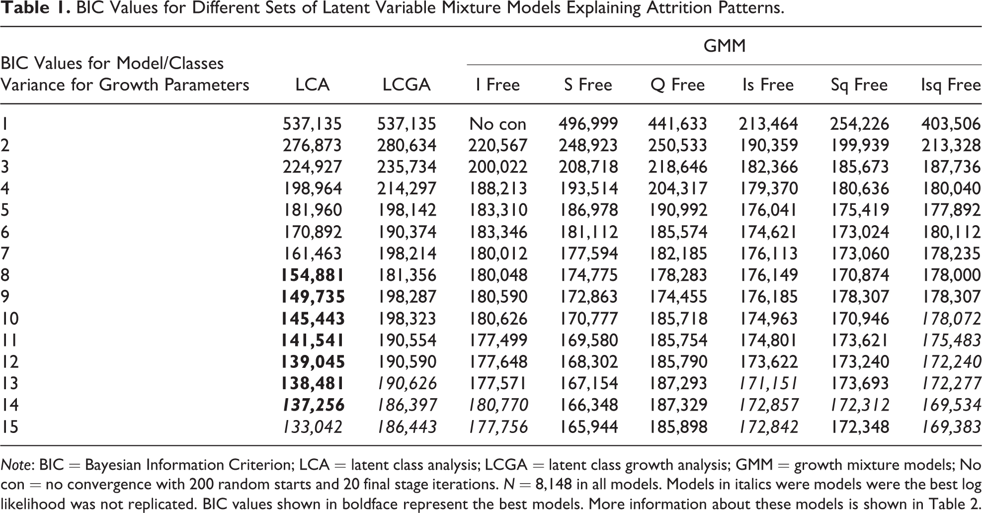
Note: BIC = Bayesian Information Criterion; LCA = latent class analysis; LCGA = latent class growth analysis; GMM = growth mixture models; No con = no convergence with 200 random starts and 20 final stage iterations. N = 8,148 in all models. Models in italics were models were the best log likelihood was not replicated. BIC values shown in boldface represent the best models. More information about these models is shown in Table 2.

For the seven models with the lowest BIC values that converged (in boldface), we report more model evaluation criteria in Table 2. We report the absolute fit of the model summarized in the deviance statistic (Singer and Willett 2003), the number of free parameters (indicating model parsimony), the entropy, and do specific paired comparison tests on the model fit of the models. The LMRT and BLRT (Nylund, Asparouhov, and Muthén 2007) both test whether the model with k − 1 classes does not fit significantly worse than the model with k classes.

Table 2.

Fit Statistics and Model Fit Information of Six of the Best-Fitting Models.

Model	Number of Classes	Deviance	BIC	Number of Free Parameters	Entropy	Size of Smallest Class	Lo–Mendell–Rubin p Value	Bootstrapped Likelihood Ratio Test p Value
LCA	8	150,846	154,881	448	.980	329	.754	.000
LCA	9	145,250	149,735	498	.982	248	.106	.000
LCA	10	140,508	145,443	548	.983	260	.415	.000
LCA	11	136,144	141,541	598	.984	199	.264	.000
LCA	12	133,130	139,045	648	.982	201	.143	.000
LCA	13	132,194	138,481	698	.980	151	.322	.000
LCA	14	130,520	137,256	748	.980	0	.239	.000

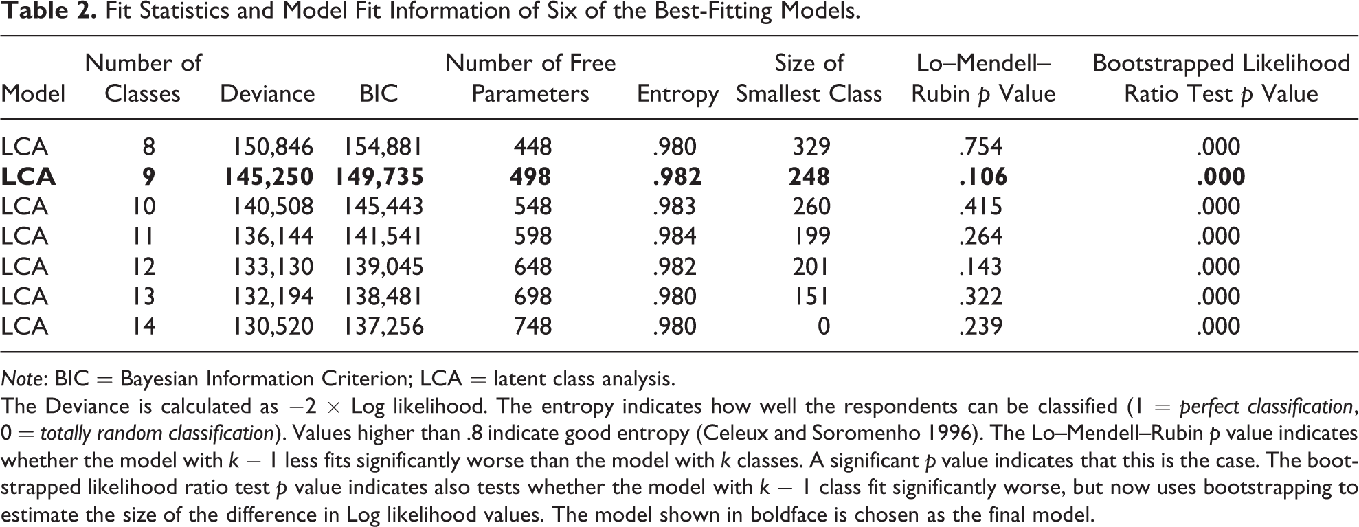
Note: BIC = Bayesian Information Criterion; LCA = latent class analysis.

The Deviance is calculated as −2 × Log likelihood. The entropy indicates how well the respondents can be classified (1 = perfect classification, 0 = totally random classification). Values higher than .8 indicate good entropy (Celeux and Soromenho 1996). The Lo–Mendell–Rubin p value indicates whether the model with k − 1 less fits significantly worse than the model with k classes. A significant p value indicates that this is the case. The bootstrapped likelihood ratio test p value indicates also tests whether the model with k − 1 class fit significantly worse, but now uses bootstrapping to estimate the size of the difference in Log likelihood values. The model shown in boldface is chosen as the final model.

It remains unclear in the literature which of these tests performs best under what circumstances (see Nylund, Asparouhov, and Muthén 2007). In Table 2, the results from both tests are rather conflicting: the LMRT test suggests that a model with seven classes does not fit worse than any of the models with more classes while the BLRT indicates we need 14 classes.

Although several models describe our data well, we chose the latent class model with nine classes as our final model. Although this model does not have the best model fit in terms of BIC, the substantive solution of this model was best interpretable. The models with 10, 11, or 12 classes introduced extra attrition classes that resembled the attrition patterns of the nine-class solution. The extra classes differed only in the exact timing of attrition. The entropy value of .98 for the nine-class solution indicates that almost all respondents can be accurately classified into one class. From now, we will discuss the results for this model only.

One of the primary advantages of latent variable models is that they allow uncertainty about model parameters. Therefore, respondents are not only assigned to one class, but class probabilities reflect the propensity to be a member of a particular attrition class. In order to show how the attrition process in the different classes takes place, we therefore discuss the posterior observed response patterns given by the model weighted for the class probabilities of every respondent.

Attrition—When and How?

Figure 1 shows the observed posterior response probabilities for each class. The first class of respondents in the panel is comprised of a group we call “loyal stayers.” This group is the largest in the panel and consists of about 37 percent of all respondents. Together with a smaller group of “slow starters” (class 2–3 percent of sample) who respond infrequently at first, but from wave 12 start to resemble the loyal stayers, these respondents participate in almost all waves of the panel. The response probabilities for the loyal stayers are between 0.90 and 1.0 in every wave of the panel, which means that at any given wave more than 90 percent of respondents participate in the survey. The group of slow starters has somewhat lower probabilities, reaching .85 around wave 14.

Figure 1.

Posterior wave response probabilities and sizes for the most likely class membership for the latent class model with nine classes.

Classes 3 to 7 all consist of respondents who follow a classic pattern of attrition. All groups start off responding very frequently, but at some point in the panel, their response probabilities decline until they all drop out of the survey. The attrition in these classes results in response probabilities that reach 0, implying that no one in these classes participates anymore. The classes differ in the timing of dropout. The third class (5 percent of sample) drops out around wave 40. Class 4 (5 percent of sample) drops out around wave 30, class 5 (9 percent of sample) drops out around wave 18, while class 6 (9 percent of sample) drops out around 12 of the panel. Finally, class 7 (19 percent of sample) consists of respondents who drop out right from the start of the panel. By wave 8 of the study, all respondents in this class have left the study.

The two remaining classes of respondents consist of respondents who do not follow a typical pattern of attrition. Rather, these respondents respond infrequently from the start of the panel and continue this response behavior over the course of the panel. Class 8 represents respondents who have slow declining response probabilities at the start of the panel, and then stabilize around .70. Because of their infrequent response behavior, we label this class “high lurkers.” This separates them from the class of “low lurkers”, who have response probabilities between .40 and .60.

Figure 1 also shows why the parametric attrition models did not fit the data as well as the latent class models for which we show the results here. The response patterns in several classes do not follow a linear trend. For example, response probabilities are in all classes lower in wave 1 and wave 6 than at other waves. In wave 1, we attribute that to the fact that some respondents were still in the process of setting up their panel membership. We believe response probabilities in wave 6 are lower because of the fact that the invitation announced that a complicated questionnaire on income and assets was to be filled out. We hypothesize that many respondents did not feel like giving details on this topic. From Figure 1, we can also see that after wave 6, the response propensities really start to vary: Loyal stayers all respond again in the next waves, but in several attriting classes this is not the case. We come back to this observation in the discussion.

The Characteristics of Attriters

We will now describe how each of the nine latent classes differ on the covariates which were used to predict respondent classification into latent classes. The coefficients shown in Table 3 represent the logit values of being in classes 2 to 9 versus being in class 1 (loyal stayers). We favor the use of logit parameters over odds ratios to be able to compare the predictive power of every covariate.⁶

Table 3.

Unstandardized Growth Parameters and Multinomial Regression Coefficients (Logit) of the Covariates (X) on Class Membership (c).

	Class 1	Class 2	Class 3	Class 4	Class 5	Class 6	Class 7	Class 8	Class 9
	Loyal Stayers	Slow Start	40 Months	30 Months	18 Months	12 Months	Fast	High Lurkers	Lurkers
Logit coefficients/covariates
Sociodemographic
Gender (1 = f)	—	−.15 (.17)	−.05 (.15)	.15 (.13)	.12 (.11)	.22 (.11)*	−.05 (.07)	.22 (.13)	.00 (.15)
Age	—	−.05 (.01)**	−.02 (.01)**	−.01 (.01)**	−.03 (.00)**	−.02 (.00)**	−.03 (.00)**	−.04 (.00)**	−.05 (.01)**
Income (13 cat)	—	.03 (.06)	−.07 (.04)	−.05 (.04)	.07 (.03)*	.07 (.03)**	.09 (.02)**	.07 (.03)*	.09 (.05)*
Education (7 cat)	—	−.31 (.07)**	−.08 (.05)	−.04 (.05)	−.11 (.04)**	−.07 (.03)*	−.09 (.03)**	.06 (.05)	−.06 (.05)
Urbanicity	—	−.02 (.05)	.04 (.06)	−.01 (.05)	−.02 (.04)	−.05 (.04)	−.06 (.04)	−.06 (.04)	−.09 (.06)
Partner(1 = yes)	—	.03 (.17)	.06 (.16)	−.18 (.15)	−.04 (.12)	.15 (.12)	.32 (.10)**	.21 (.13)	.32 (.18)
SimPC (1 = yes)	—	.32 (.28)	.02 (.33)	−1.11 (.44)*	−1.16 (.38)**	−.72 (.30)*	−.71 (.24)**	.01 (.29)	.18 (.49)
Psychological
Openness	—	−.10 (.09)	−.08 (.09)	−.02 (.08)	.01 (.07)	.19 (.07)**	−.01 (.04)	.04 (.08)	−.01 (.11)
Conscientiousness	—	.02 (.08)	−.04 (.08)	−.09 (.07)	−.07 (.05)	−.06 (.05)	−.11 (.03)**	−.21 (.06)**	−.23 (.07)**
Extraversion	—	.05 (.08)	.27 (.08)**	.10 (.07)	.12 (.07)	.17 (.06)**	.28 (.04)**	.16 (.07)*	.26 (.07)**
Agreeableness	—	.01 (.07)	−.04 (.09)	−.15 (.07)*	.09 (.06)	.02 (.06)	.12 (.04)**	.19 (.08)*	.10 (.08)
Neuroticism	—	.14 (.08)	−.04 (.08)	−.05 (.07)	−.01 (.05)	−.06 (.06)	.06 (.04)	.07 (.06)	.01 (.07)
Need to evaluate	—	.00 (.08)	−.07 (.08)	−.07 (.08)	−.11 (.06)	−.13 (.06)*	−.22 (.04)**	−.19 (.06)**	−.14 (.08)
Need for cognition	—	.11 (.10)	.14 (.09)	.08 (.08)	.06 (.07)	−.17 (.07)**	.07 (.04)	.11 (.08)	.19 (.11)
Survey attitude
1. Enjoy Internet	—	−.14 (.07)	−.21 (.05)**	−.19 (.05)**	−.21 (.04)**	−.26 (.04)**	−.23 (.04)**	−.08 (.04)*	−.09 (.06)
2. Enjoy—interviewed	—	.11 (.06)	.01 (.04)	.08(.04)	−.05 (.03)	−.09 (.03)**	−.01 (.03)	−.03 (.04)	.03 (.05)
3. Interesting	—	−.09 (.08)	−.09 (.05)	−.09 (.05)	−.10 (.04)*	−.13 (.04)**	−.09 (.04)*	−.05 (.05)	.07 (.07)
4. Important	—	−.03 (.09)	−.03 (.06)	.11 (.06)	.01 (.05)	−.04 (.05)	.07 (.05)	−.03 (.05)	−.21 (.07)**
5. A lot can be learned	—	.07 (.09)	.01 (.06)	−.09 (.06)	.01 (.05)	.02 (.05)	−.02 (.05)	.04 (.06)	.04 (.07)
6. Waste of time	—	.03 (.07)	−.04 (.06)	−.06 (.05)	−.01 (.04)	.04 (.04)	.08 (.03)**	.10 (.04)	.00 (.05)
7. Too many requests	—	.02 (.05)	.01 (.04)	−.02 (.04)	.01 (.03)	−.00 (.03)	−.01 (.02)	−.02 (.03)	.01 (.04)
8. Privacy concerns	—	.08 (.05)	−.04 (.04)	−.00 (.04)	.05 (.03)	.08 (.03)**	.01 (.03)	−.00 (.04)	−.02 (.05)
9. Exhaustive	—	.11 (.05)*	.06 (.04)	.06 (.04)	.10 (.03)**	.12 (.03)**	.09 (.02)**	.09 (.04)*	.03 (.04)

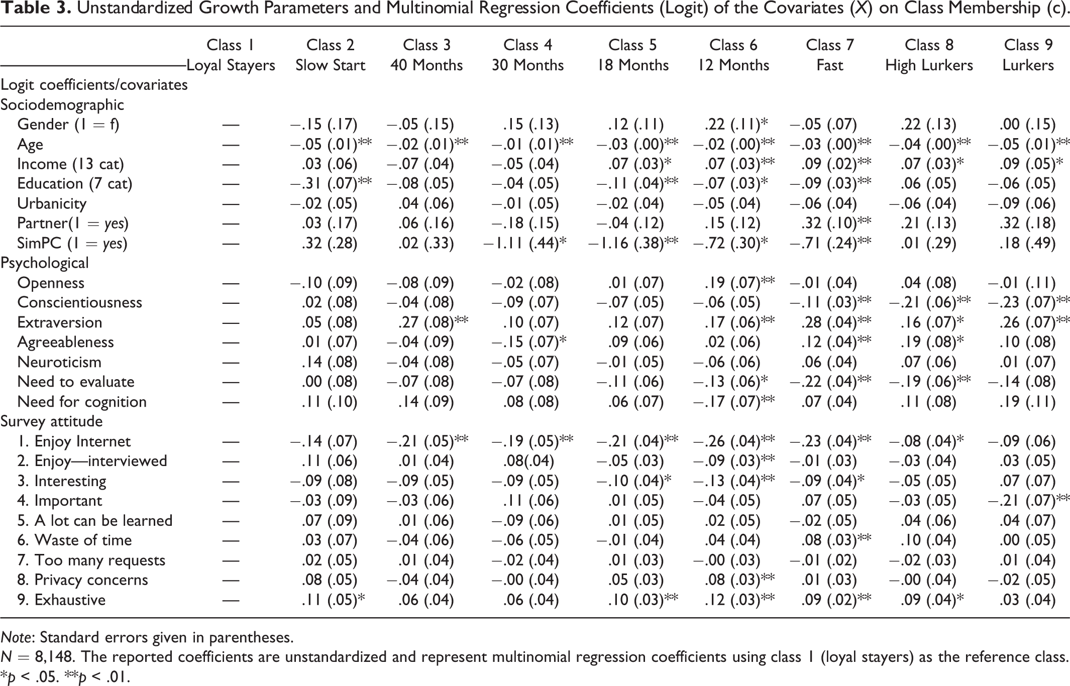
Note: Standard errors given in parentheses.

N = 8,148. The reported coefficients are unstandardized and represent multinomial regression coefficients using class 1 (loyal stayers) as the reference class.

*p < .05. **p < .01.

First, we look at the sociodemographic predictors. Surprisingly, we do not find that males attrite more often than women. The logit parameter of −.15, for example, means that compared to the class of loyal stayers, we find the proportion of females to be .15 log odds lower in the class of slow starters. This translates into an odds ratio of 0.87, holding all other variables constant. Compared to the class of stayers, we only find more males in the class who attrites after 12 months.

In all attriting classes, we find younger people compared to the loyal stayers, and we find the largest difference for the slow starters and both classes of lurkers. People in all classes (2 to 9) have a lower education than people in the class of loyal stayers, while urbanicity and having a partner are not predictive of class membership. Finally, having a SimPC strongly predicts not dropping out in the survey, as can be seen in the relatively large coefficients in all attriting classes, apart from the class who drops out around 40 months into the study. For the slow starters and lurkers, we find no effect of having a SimPC on attrition.

With the psychological variables, we can more directly evaluate whether we find the attrition processes to correspond with theories on the causes of attrition. We find the stayers to differ very little from the slow starters, and those groups who dropout late in the panel study (at 40, 30, and 18 months). We do find the groups who attrite early (at 12 months and the fast drop-out class), to score higher on extraversion, and lower on the need to evaluate. The group of fast attriters in particular has a very different psychological profile: They are more agreeable and less conscientious. Lurkers resemble the group of fast attriters quite closely. Lurkers are less conscientious and more extravert than loyal stayers.

The psychological variables have the largest logit parameters, thus explaining the differences between the attrition classes best. The survey attitude questions also predict latent class membership, but we find only one of the survey questions to be highly predictive. Loyal stayers enjoy completing Internet surveys far more than respondents in all other classes. We find the stayers also to be more positive on other questions, but the differences between the classes are often not significant.

In summary, the loyal stayers are more conscientious, less extraverted, less agreeable, older, more educated, and enjoy Internet surveys survey more than the classes of lurkers and those respondents who drop out in the first year of the panel study. Also, having been given a SimPC is predictive of not attriting before wave 40, although we find people with a SimPC in the groups of lurkers. The two classes of lurkers stand out as being a lot younger than respondents in other classes, but lurkers report that they do enjoy completing surveys. All people who drop out at some point report not enjoying Internet surveys as much as the loyal stayers.

Almost all these findings are in line with the commitment hypothesis. Fast attriters are less conscientious and have a lower need to evaluate than the stayers, which implies that attriters are less committed to being a good panel respondent. Also, respondents who drop out in the first two years enjoy completing surveys less.

Attrition—Does It Matter?

Apart from looking at the characteristics of those who attrite, it is also interesting to see how attrition matters for substantive statistics. Here we focus on how the different attrition classes are correlated with the estimate of the Dutch parliamentary election results in 2006. We chose the variable voting behavior on purpose, as we can validate the survey estimates using all respondents in the panel, the respondents in the various attrition classes and those who remain in the panel at wave 48. Voting behavior was recorded twice in the first waves of the panel, so we have information for most of the panel members.⁷

Table 4 shows the actual election results (in percentages) for the general election in the second column. The third and fourth columns show the results for the respondents in the LISS panel at waves 1 and 48 of the panel. We see that bias already exists at the start of the panel, most likely due to nonresponse in the panel recruitment phase, although some measurement errors should not be excluded as a potential cause. At the start of the panel, the absolute bias adds up to 9.3 percentage points when compared to the official result. Forty-seven months later, using only the people who are still active at the end of our study, attrition bias has decreased to 6.7 percentage points.

Table 4.

Estimates of the Election Result and the Contribution to Nonresponse Bias of Every Attrition Class.

Party/Voting Percentages	Election Results	Wave1	Wave 48	1	2	3	4	5	6	7	8	9
Chr. Dem. (CDA)	26.5	25.3	26.5	26.3	12.9	21.3	25.8	28.9	25.6	20.5	26.1	24.9
Labor (PvdA)	21.2	19.3	20.6	20.4	19.4	16.3	17.8	17.8	19.4	21.3	18.8	20.3
Socialists (SP)	16.6	17.2	17.7	17.8	19.4	19.8	16.7	17.2	15.6	18.1	16.3	15.3
Liberals (VVD)	14.7	15.7	15.7	15.0	19.4	18.6	14.4	14.1	17.1	17.2	18.4	13.0
Freedom (PVV)	5.9	4.4	3.4	3.5	6.5	6.5	6.1	4.8	4.8	4.9	2.9	5.6
Green Left (GL)	4.6	6.4	4.4	4.6	6.5	4.9	7.2	8.1	8.3	8.1	6.6	6.8
Chr. Union (CU)	4.0	5.0	5.1	5.3	3.2	3.4	7.2	3.5	3.5	5.2	4.1	6.2
Others	6.5	6.8	6.7	7.0	12.9	9.1	4.9	5.5	5.6	7.1	6.8	7.9
Absolute bias	—	9.3	6.7	6.7	—	21.3	12.1	13.1	12.3	16.4	12.2	11.6
Percentage contribution	—	—		26.2	—	10.2	5.8	10.9	10.8	22.5	9.8	3.8

Note: N = 4,998. This includes all panel members who responded in January 2008 (wave 1). The names of the political parties are translated and abbreviated. For the original names, see www.lissdata.nl. Column 2 denotes the true parliamentary results. Column 3 represents the election result estimated with the data as provided by respondents in wave 1, thus only including initial nonresponse bias. The fourth column denotes the same estimate, but only using the respondents who responded to wave 48. The fifth to fourteenth columns denote the estimate of the election results, using only respondents in those specific classes. Because of a small sample size, the bias contributions for class 2 are not shown. All results are unweighted for initial sample selection probabilities and nonresponse in the panel recruitment phase. The absolute bias indicates the bias in each class or wave as compared to the official election result, unweighted for class size (sum of all party biases). The percentage contribution shows the contribution of each class in the total absolute Nonresponse bias, weighted for the size of each class.

The 5th to 14th column show estimates for the election results in every class, as well as the absolute difference (summed) with the official election result. We see that the difference between the election results and the class-based estimate of the election results is large in the class of respondents who drops out after 40 months (absolute difference of 21 percent) and the fast attriters (16 percent). This means that attrition is selective with regard to voting behavior. However, this selectivity in voting behavior estimates for the attrition classes leads to an overall reduction in bias, meaning that the selectivity in voting behavior for attriting classes corrects for some of the bias that was introduced during the panel recruitment process.

Conclusion and Discussion

This article showed how attrition can be described as a process that varies over individuals and time. Almost all of the respondents in our study miss one or more waves of the study. Sometimes, wave nonresponse leads to permanent dropout, but more often, respondents return to the panel survey.

At every wave, respondents have an unobserved response propensity that allows us to distinguish several classes of respondents who follow a different attrition process. The analysis model that we propose corresponds to substantive theories about attrition and overcomes analytical problems in previous attrition studies. The group of “ever out” respondents is diverse and consists of stayers, late and fast attriters and lurkers. These groups differ from each other not only in their response patterns but also substantively. Attriters have a different type of personality and value survey participation differently from loyal stayers. Our results suggest that attriters have less commitment and higher levels of panel fatigue.

Apart from commitment and panel fatigue, habit and shock are the other hypothetical causes of attrition. Although we cannot evaluate these causes directly, the response propensities shown in Figure 1 can be used to evaluate these causes indirectly. The response propensities in the classes of gradual and fast attriters show a sudden decline at wave 6 of the panel survey. Wave 6 was fielded in June 2008, before the summer holidays, so we have no reason to believe that many respondents were on holidays and did not read the survey invitation. We believe the shock in wave 6 to have occurred because of the topic of that month’s survey. Respondents had to report in detail about their household’s sources of income, details of their income, as well as their expenses, and could read about this in the survey invitation. The interviewing time for this topic amounted to about half an hour, which probably caused many respondents not to start that wave. Response probabilities for the class of loyal stayers drop by about 0.05 in wave 6, but for the early attrition classes, the probabilities drop by about 0.3. In the class of late attriters and loyal stayers, respondents return to the panel after wave 6, so that their response probabilities are back at around 0.9 at wave 11. For the classes who attrite after wave 12, however, this sudden drop in response probabilities is followed by total attrition over the next waves.

To evaluate the shock hypothesis more formally, we would need time-varying covariates on, for example, household situation, moving, and health status, which are beyond the scope of this article. The inclusion of time-variant covariates should not fundamentally alter the latent class model we used. Estimation of latent class models with time-variant covariates is however time consuming. Future increases in computing power should solve this problem. One would expect the time-variant covariates to have no effect on responses in the classes of loyal stayers, nor in the group of fast attriters or lurkers, as response probabilities in these classes are rather stable over time. However, they should strongly predict the timing of attrition for the classes who drop out. For them, a shock, whether it is in the form of a life event or an unpleasant panel experience, can make the balance of positive and negative survey participation factors tip firmly to the negative and lead to attrition. The response probabilities in Figure 1 do show however that complicated and boring questionnaires can either lead to direct attrition (shock) or break the habit of responding to survey requests, starting or accelerating a downward trend in response probabilities leading to attrition. This finding shows how questionnaire design and the survey process itself are very important in the attrition process.

Further analyses into attrition processes should not only focus on attrition errors, but take all survey errors into account. In this article, we explicitly chose not to study any survey errors that were introduced prior to the start of the panel. Although we want to stress the importance of the panel composition stage for limiting the size of total survey error, we here focused on the determinants of nonresponse conditional on enrolment in the survey. Ideally, any study of attrition should not only study errors because of initial nonresponse and attrition but also measurement errors. Panel managers could try to prevent or limit attrition and initial nonresponse, but if this comes at the price of lower data quality, pursuing tailoring strategies may come at a price of decreasing data quality. Research in cross-sectional surveys has suggested that more reluctant respondents also have the lowest data quality (Tourangeau, Groves, and Redline 2010). One way forward to incorporate measurement errors in attrition models is to include indicators of the response quality per class.

We only tested attrition bias for voting behavior, and the possibility remains that nonresponse bias is different for other variables. For the LISS panel, it seems that the bias that was introduced at the start of the panel actually decreases with time. However, attrition bias does exist in the class of loyal stayers, who with time will comprise an increasingly large proportion of the panel, possibly leading to more bias with time. It is therefore important to try and prevent those at risk from dropping out of the panel survey.

The final question that remains unanswered is whether attrited respondents in the LISS panel have really dropped out forever. Many respondents miss out on one or more waves toward the end of our study. This study focuses only on original sample members, but in 2010, new top-up samples were added to the panel. At the same time, attrited panel members were attempted to be reactivated. A different study (Lugtig, Das, and Scherpenzeel, 2014) showed that many reactivated respondents only stayed in the panel for a short period, after which they dropped out again. Another suggestion for future research that follows from this study is that incentives could be tailored to specific respondents. Loyal Stayers may not need extra feedback or information about the panel to keep them active, but lurkers and attriters may be activated by providing incentives in the form of extra information about the panel, thank-you cards, or even monetary incentives.

Footnotes

Acknowledgment

I would like to thank Joop Hox and Edith de Leeuw, Thomas Klausch, and Anja Boevé and participants to the panel survey methods and nonresponse workshops for their comments on earlier versions of this article. I would also like to thank Annette Scherpenzeel and CentERdata for providing me with data and being supportive of my work. Finally, I thank two anonymous reviewers for their comments on an earlier version of this article.

Declaration of Conflicting Interests

The author(s) declared no potential conflicts of interest with respect to the research, authorship, and/or publication of this article.

Funding

The author(s) disclosed receipt of the following financial support for the research, authorship, and/or publication of this article: UK Economic and Social Research Council (grant number ES/K001027/1).

Notes

References

AAPOR (American Association for Public Opinion Research). 2009. Standard Definitions: Final dispositions of case codes and outcome rates for surveys. 6th ed. Kansas: AAPOR.

Behr

Bellgardt

Rendtel

. 2005. “Extent and Determinants of Panel Attrition in the European Community Household Panel.” European Sociological Review 21:489–512.

Bizer

G. Y.

Krosnick

J. A.

Holbrook

A. L.

Wheeler

S. C.

Rucker

D. D.

Petty

R. E.

. 2004. “The Impact of Personality on Cognitive, Behavioral, and Affective Political Processes: The Effects of Need to Evaluate.” Journal of Personality 72:995–1028.

Cacioppo

J. T.

Petty

R. E.

. 1983. “Effects of Need for Cognition on Message Evaluation Recall and Persuasion.” Journal of Personality and Social Psychology 45:805–18.

Celeux

Soromenho

. 1996. “An Entropy Criterion for Assessing the Number of Clusters in a Mixture Model.” Journal of Classification 13:195–212.

Costa

Paul

McCrae

R. R.

. 1992. “Normal Personality Assessment in Clinical Practice: The NEO Personality Inventory.” Psychological Assessment 4:5–13.

Davidov

Yang-Hansen

Gustafsson

Schmidt

Bamberg

. 2007. “Does Money Matter? A Theory-driven Growth Mixture Model to Explain Travel-mode Choice with Experimental Data.” Methodology 2:124–34.

Durrant

G. B.

Goldstein

. 2010. “Analysing the Probability of Attrition in a Longitudinal Survey.” Working Paper, (M10/08), University of Southampton, Southampton, England.

Feldman

B. J.

Masyn

K. E.

Conger

R. D.

. 2009. “New Approaches to Studying Problem Behaviors: A Comparison of Methods for Modeling Longitudinal, Categorical Adolescent Drinking Data.” Developmental Psychology 45:652–76.

10.

Fitzgerald

Gottschalk

Moffitt

. 1998. “An Analysis of Sample Attrition in Panel Data: The Michigan Panel Study of Income Dynamics.” Journal of Human Resources 33:251–99.

11.

Goldberg

L. R.

Johnson

J. A.

Eber

H. W.

Hogan

Ashton

M. C.

Cloninger

C. R.

Gough

H. C.

. 2006. “The International Personality Item Pool and the Future of Public Domain Personality Measures.” Journal of Research in Personality 40:84–96.

12.

Hill

D. H.

Willis

R. J.

. 2001. “Reducing Panel Attrition: A Search for Effective Policy Instruments.” The Journal of Human Resources 36:416–38.

13.

Jarvis

W. B. G.

Petty

R. E.

. 1996. “The Need to Evaluate.” Journal of Personality and Social Psychology 70:172–94.

14.

Jones

A. M.

Koolman

Rice

. 2006. “Health-related Non-response in the British Household Panel Survey and European Community Household Panel: Using Inverse-probability-weighted Estimators in Non-linear Models.” Journal of the Royal Statistical Society Series A 169:543–69.

15.

Kreuter

Muthén

. 2008. “Longitudinal Modeling of Population Heterogeneity: Methodological Challenges to the Analysis of Empirically Derived Criminal Trajectory Profiles.” Pp. 53–75 in Advances in Latent Variable Mixture Models, edited by Hancock

C. R.

Samuelson

K. M.

. Charlotte, NC: Information Age Publishing.

16.

Laurie

Smith

Scott

. 1999. “Strategies for Reducing Nonresponse in a Longitudinal Panel Survey.” Journal of Official Statistics 15:269–82.

17.

Leenheer

Scherpenzeel

. 2011. “Does It Pay Off to Include Non-internet Household in an Internet Panel?” International Journal of Internet Science 8. Retrieved July 2, 2013 (http://www.ijis.net/ijis8_1/ijis8_1_leenheer_and_scherpenzeel_pre.html).

18.

Leeuw

E. D.

Hox

J. J.

Lugtig

Vis

Göritz

Bartsch

Engel

. 2010. “Does Familiarity Breed Contempt? Measuring and Comparing Survey Attitude among New and Repeat Respondents Cross-culturally.” Paper presented at the 63rd WAPOR Conference, May 13, Chicago, IL.

19.

Lemay

2010. “Understanding the Mechanism of Panel Attrition.” Unpublished Doctoral thesis, Doctor of Philosophy, University of Maryland, College Park, MD.

20.

Lepkowski

J. M.

Couper

M. P.

. 2002. “Nonresponse in the Second Wave of Longitudinal Household Surveys.” Pp. 257–72 in Survey Nonresponse, edited by Groves

Robert M.

. New York: John Wiley.

21.

Lillard

L. A.

Panis

C. W. A.

. 1998. “Panel Attrition from the Panel Study of Income Dynamics—Household Income, Marital Status and Mortality.” The Journal of Human Resources 33:437–57.

22.

Lipps

2009. “Attrition of Households and Individuals in Panel Surveys.” SOEPpapers 164. Berlin: DIW. Retrieved January 8, 2014 (http://www.diw.de/documents/publikationen/73/diw_01.c.96125.de/diw_sp0164.pdf).

23.

Loosveldt

Pickery

Billiet

. 2002. “Item Nonresponse as a Predictor of Unit Nonresponse in a Panel Survey.” Journal of Official Statistics 18:545–57.

24.

Lugtig

Das

Scherpenzeel

A. C.

. 2014. Nonresponse and attrition in a probability-based Online panel for the general population. In Callegaro

Lavrakas

P. J.

Krosnick

J. Baker

Reginald

Bethlehem

Göritz

A. S.

(Eds). Online panel research: A data quality perspective. Wiley series in survey methodology, New York: Wiley.

25.

Muthén

. 2006. “The Potential of Growth Mixture Modeling.” Infant and Child Development 15:623–25.

26.

Muthén

. 2010. Bayesian Analysis in Mplus: A Brief Introduction. Version 3. Los Angeles, CA: Muthen & Muthen.

27.

Muthén

L. K.

Muthén

. 2010. MPLUS User’s Guide. Los Angeles, CA: Muthén & Muthén.

28.

Muthén

L. K.

Muthén

. 2013. MPLUS 7.11. Los Angeles, CA: Muthén & Muthén.

29.

Nicoletti

Peracchi

. 2005. “Survey Response and Survey Characteristics: Microlevel Evidence from the European Community Household Panel.” Journal of the Royal Statistical Society Series A 168:763–81.

30.

Nylund

K. L.

Asparouhov

Muthén

. 2007. “Deciding on the Number of Classes in Latent Class Analysis and Growth Mixture Modeling: A Monte Carlo Simulation Study.” Structural Equation Modeling 14:535–69.

31.

Rogelberg

S. G.

Fisher

G. G.

Maynard

D. C.

Hakel

M. D.

Horvath

. 2001. “Attitudes toward Surveys: Development of a Measure and Its Relationship to Respondent Behavior.” Organizational Research Methods 4:3–25.

32.

Singer

J. D.

Willett

J. B.

. 2003. Applied Longitudinal Data Analysis—Modeling Change and Event Occurrence. New York: Oxford University Press.

33.

Stocké

. 2006. “Attitudes Toward Surveys, Attitude Accessibility and the Effect on Respondents’ Susceptibility to Nonresponse.” Quality and Quantity 40:259–88.

34.

Tabachnick

B. G.

Fidell

L. S.

. 2007. Using Multivariate Statistics. 5th ed. New York: Pearson Education.

35.

Tortora

R. D

. 2009. “Attrition in Consumer Panels.” Pp. 235–48 in Methodology of Longitudinal Surveys, edited by Lynn

. Chichester, England: John Wiley.

36.

Tourangeau

Groves

R. M.

Redline

C. D.

. 2010. “Sensitive Topics and Reluctant Respondents. Demonstrating a Link between Nonresponse Bias and Measurement Error.” Public Opinion Quarterly 74:413–32.

37.

Tuten

T. L.

Bosnjak

. 2001. “Understanding Differences in Web Usage: The Role of Need for Cognition and the Five Factor Model of Personality.” Social Behavior and Personality 29:391–98.

38.

Uhrig

S. N

. 2008. “The Nature and Causes of Attrition in the British Household Panel Survey.” ISER Working Paper, 5. Colchester, England: Institute for Social and Economic Research.

39.

Voorpostel

2009. “Attrition in the Swiss Household Panel by Demographic Characteristics and Levels of Social Involvement.” FORS Working Paper, 1_09. Lausanne, Switzerland: Swiss Foundation for Research in Social Sciences. Retrieved January 8, 2014 (http://aresoas.unil.ch/workingpapers/WP1_09.pdf).

40.

Watson

Wooden

. 2009. “Identifying Factors Affecting Longitudinal Survey Response.” Pp. 157–82 in Methodology of Longitudinal Surveys, edited by Lynn

. Chichester, England: John Wiley.