Increasing Inferential Leverage in the Comparative Method

Introduction

The use of comparison to determine whether an explanatory factor X affects some outcome Y in a pair or small number of cases features prominently in the social sciences (Collier 1993). These studies generally select cases to be as similar as possible on the important control variables and have different values of the key explanatory variable. They then examine whether the outcome differs across the cases, appealing to Mill’s (1872) method of difference, the most similar or most similar systems design (Przeworski and Teune 1970), the comparable-cases strategy or the comparative method (Lijphart 1971, 1975). But these methods are problematic in several ways. As Lieberson (1991, 1994) and Sekhon (2004) point out, Mill’s methods for small-n comparisons require determinism, absence of measurement error, preclusion of other possible causes of the effect of interest, and lack of interaction effects for valid inferences. Because most social and political processes are unlikely to meet these stringent conditions, Sekhon suggests moving to a probabilistic framework and to a large-n study in which statistical methods can be applied. This is similar to King, Keohane, and Verba’s (1994) prescription for adapting a small-n analysis into a large-n analysis at the subunit level.

But this solution may not be desirable or possible. For a variety of reasons, one may be interested in particular cases or even a specific case, as for case-oriented comparative research (Ragin 1987), but a move to large-n typically changes the study’s goal from a causal effect for a particular unit to an average causal effect for many units. Similarly, the move to a subunit analysis typically changes the study’s goal from a causal effect for that unit to an average causal effect for many subunits. The move to large-n may also not be feasible, since the cases available for a large-n study with differing values of the explanatory variable may not be very similar on the control variables (Brady 2004:53; Brady and Collier 2004; Munck 2004:113). After reducing the analysis to those matching cases that are sufficiently similar, we may only have enough cases for a small-n study. When can the comparative method provide leverage for inferring the causal effect of X on Y for these cases in small-n studies, and how should we select our cases for comparison in order to exploit this method?

Confidence in conclusions drawn using any method depends upon the validity of the assumptions underlying the method. We therefore make explicit the homogeneity assumption required for the comparative method, distinguish the comparative method from Mill’s method of difference, and delineate its three procedural variants. In other words, we lay out the methodology of the comparative method (Lijphart 1975). With this framework, we demonstrate that even if our goal is inference only for the two units being compared and not a larger population, additional units can provide what is sometimes known as a “placebo test” (Abadie, Diamond, and Hainmueller 2010, 2011). In the most general usage of the term, a placebo test is a secondary test that uses the same logic and preconditions as the primary test, but where it is known that there is no effect. Hence, the placebo test should not detect an effect. If the placebo test detects a nonexistent effect, then we should be skeptical of the evidence from the primary test. The use of the homogeneity assumption in the comparative method means that these placebo tests may be available even when the two units being compared are the most similar pair of units on the control variables with differing values of the explanatory variable. Furthermore, these additional units beyond the scope of inference may have the same value of the explanatory variable X. To our knowledge, this point has never been stated explicitly, although it is implicit in the placebo tests of Abadie, Diamond, and Hainmueller (2010) and the placebo tests and p-values suggested in Abadie, Diamond, and Hainmueller (2011) and implied by analogous large-n placebo tests. ¹ We elaborate on the exact methods for using these additional units through examples and a formal discussion in the following sections.

This surprising source of inferential leverage suggests several changes to current practice for small-n studies using the comparative method. First, studies that employ the comparative method should consider using additional units beyond those being compared, since comparing one selectively chosen unit to a primary case of interest does very little to strengthen inference. If it is too difficult or costly to assess additional cases beyond the comparison case, then the most appropriate form of analysis may be careful process tracing (Gerring 2007:chap. 7), or other methods for establishing the effect of X on Y in that main case. ² Researchers should not include a second case that adds little to the study, unless it can be used to justify the homogeneity assumption.

At a minimum, researchers using the comparative method should provide the details necessary for future studies on additional units to provide this supplementary leverage, since the comparisons add little to our confidence in the analysis without these details. Researchers need not conduct numerous additional case studies themselves. But they should provide a road map, so that other scholars may assess the validity of these comparisons—a new way in which scholars who have deep expertise in cases and regions of the world beyond a study’s scope of inference can build on and contribute to that analysis in a cumulative, scientific manner. This means that small-n analyses using the comparative method must first clearly define the dependent, independent, and control variables such that they may be measured for additional units and also specify how the control variables are weighted in defining similarity between units. To this end, we propose a “list, measure, scale, and weight” standard.

Second, the strong assumptions necessary for simultaneously generating and testing theory are unlikely to be satisfied for most social science problems. This means that without specifying the theory prior to the analysis, a contrast with a second case using the comparative method cannot add confidence to our inference for the main case. Therefore, theory testing should be more clearly separated from theory generation than is the usual practice for studies employing the comparative method. The theory may be generated from the intensive study of the primary case of interest, but without inspection of other cases that may be used for testing.

Not all small-n comparisons use the comparative method for causal inference, and other small-n methods that may be employed for other goals like theory generation are beyond the scope of this article (Collier 1993; Ragin 1987). Other types of small-n comparative studies include the “parallel demonstration of history,” in which a set of case studies substantiates the applicability of a general theory in different contexts, and the “contrast of contexts,” in which the case studies focus on how unique features of each case affect the way in which general social processes transpire (Skocpol and Somers 1980). Our discussion also does not apply to comparisons of causal effects that have been established by other means; it applies only to comparisons that are intended to establish or help establish causal effects. ³

The article proceeds as follows. The second section describes two methods for small-n comparisons—the method of difference (Mill 1872) and the comparative method (Lijphart 1975)—and shows that there are three variants of the comparative method: most similar pair, most similar contrasting case, and sufficiently similar contrasting case. The third section elaborates our main points in a stylized example using the most similar pair design. The fourth section then presents a formal discussion of the comparative method as described by Lijphart (1975), including its assumptions, the implications of these assumptions for inferential leverage, and the relationship between this presentation and previous methodological discussions of Mill’s method of difference (Lieberson 1991, 1994; Sekhon 2004). The fifth section demonstrates the inferential leverage gained from additional units when the comparative method is used to find a “most similar” contrasting case to a specific case of interest by revisiting the Canada–U.S. comparison in Epstein (1964). The sixth section applies our proposed standards and these methods when there is a “sufficiently similar” contrasting case to a specific case of interest by reexamining the comparison of China with Japan in Moore’s Social Origins of Dictatorship and Democracy (1966).

Method of Difference and Comparative Method

One of the most important uses of comparison in both large-n and small-n studies is to establish causal effects. While having a large number of units may alleviate some of the difficulties of causal inference (King et al. 1994), particularly if a treatment is randomly assigned, there may be circumstances in which comparing a small number of units is necessary or even advantageous (Collier 1993; Lijphart 1975; Skocpol and Somers 1980). A number of methods have been proposed for such small-n comparisons, and a large portion of these methods involve the comparison of two units with different values of an independent variable. These methods are variously known as the method of difference (Mill 1872), most similar design (Przeworski and Teune 1970), the comparable-cases strategy (Lijphart 1975), and the comparative method (Lijphart 1971), among others.

Although these methods are often discussed as equivalent (Gerring 2007; Lijphart 1975; Przeworski and Teune 1970; Sekhon 2004), there is some ambiguity regarding the exact procedures for each method. This is problematic because different procedures require different assumptions. Take John Stuart Mill’s canonical statement of the method of difference (Mill 1872:452) to start:

If an instance in which the phenomenon under investigation occurs, and an instance in which it does not occur, have every circumstance in common save one, that one occurring only in the former; the circumstance in which alone the two instances differ is the effect, or the cause, or an indispensable part of the cause, of the phenomenon.

Contrast this with the comparative method, most directly stated by Lijphart (1975:164):

… the amount of variance of the dependent variables should not be a consideration in the choice of cases because this would prejudge the empirical question. The comparative method can now be defined as the method of testing hypothesized empirical relationships among variables on the basis of the same logic that guides the statistical method, but in which the cases are selected in such a way as to maximize the variance of the independent variables and to minimize the variance of the control variables. [emphasis in original]

Furthermore, Lijphart’s statement is an ideal and does not capture the full range of practice with the comparative method. In some applications, one of the cases is preselected because that case is of particular interest, and the comparative method is used to select the most similar contrasting case (Nielsen 2011). The two cases may not be the pair that “minimizes the variance of the control variables” for such applications. In other applications, the control variables may be difficult to measure for all possible contrasting cases. A contrasting case then cannot be known to be “most similar,” and consequently, the implicit claim is that the contrasting case is sufficiently similar for a meaningful comparison. Therefore, Lijphart’s comparative method in fact encompasses three different case selection methods: most similar pair, most similar contrasting case, and sufficiently similar contrasting case.

A Stylized Example

We now illustrate placebo tests for the comparative method through a hypothetical study of landlocked African countries on the effect of British versus French colonial history on economic growth. In our example, we measure growth as the change in gross domestic product per capita (purchasing power parity [PPP]) for the first and last year of data availability in the Bates Africa data set and dichotomize this to positive or negative growth. ⁵ We denote the identity of the colonial power with X (X = 1 for British and X = 0 for French) and economic growth with Y (Y = 1 for positive growth and Y = 0 for negative growth). For this example, we use only two hypothetical control/matching variables: the percentage of the population that is Muslim (M ₁) and the log of average rainfall (M ₂). These are presented in a scatterplot in Figure 1a, so we can visually inspect our data for countries with different values of X that are similar on the control/matching variables. Countries with British colonial history (X = 1) are represented by circles, while countries with French colonial history (X = 0) are represented by triangles.

OPEN IN VIEWER

Figure 1.

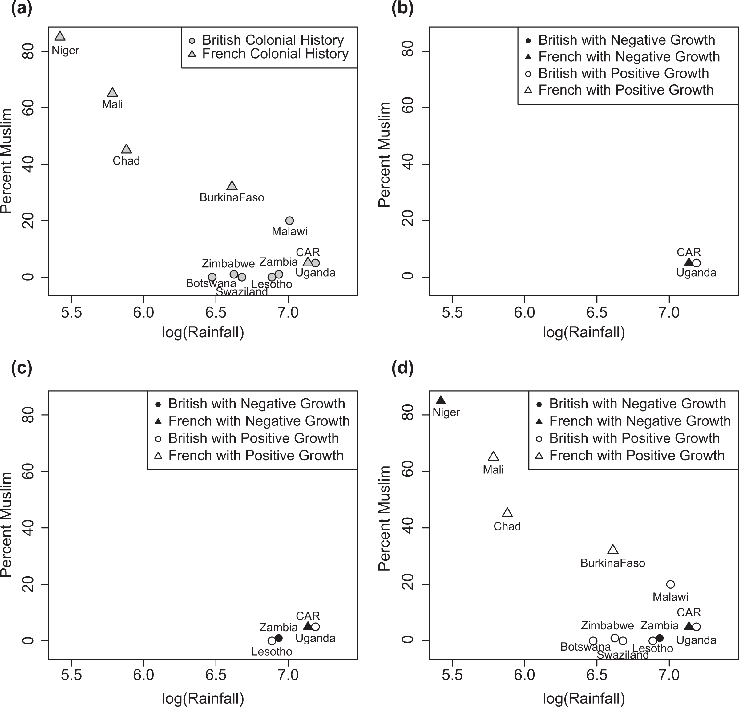
A stylized example for the effect of British or French colonial history on economic growth.

A number of elements in this example are quite stylized. First, we would certainly want to control for additional variables. This example is simple for illustrative purposes, but as with any matching analysis, we must assume that we have measured and controlled for the appropriate variables. Unmeasured confounding or controlling for the wrong set of measured variables can lead to incorrect inferences.

Second, with the exception of logging rainfall, the variables have not been recoded to accurately reflect similarity between the cases. For example, a 20 percentage point increase in the share of the population that is Muslim may have different effects for countries with Muslim populations above and below 50 percent. Third, we have not adjusted the weighting of the variables, which would be reflected in distances in the figure. In this presentation, a change of .5 in the log of average rainfall (M ₂) covers approximately the same distance as a 20-point change in the percentage of the population that is Muslim (M ₁). They indicate approximately equivalent differences in similarity, which may not accurately depict the relative importance of rainfall for economic growth. ⁶ We have also assumed that the definition of similarity is constant across the space in Figure 1a. For example, although Uganda and the Central African Republic (CAR) have more rainfall, we have implicitly assumed that Lesotho and Zambia are as similar as Uganda and the CAR. These decisions were made to simplify the presentation and discussion. Analogous decisions must be made and explained in any application, although these decisions are likely to be more nuanced in a proper study. If similarity should be judged differently for different levels of rainfall or any other variable, then this must be stated explicitly.

Let us stipulate to the accuracy of Figure 1a in representing similarity/dissimilarity between cases. First note that there are almost no cases of former British colonies that are similar to former French colonies in the values of the control/matching variables. The only former British and former French colonies that are near one another are Uganda (British, X = 1) and the CAR (French, X = 0), so that the only comparison that might reasonably be made “controlling” for the share of the population that is Muslim and average rainfall is between these two countries. In the terminology of matching, there is almost no overlap between the former British colonies and the former French colonies. Hence, this example presents the prototypical scenario for an n = 2 study with the comparative method. Proceeding with this approach, in Figure 1b, we have removed all the other countries and indicated values of the outcome variable on the plot, with open symbols representing positive growth and solid symbols representing negative growth. We see that economic growth is positive for Uganda (Y = 1) and negative for the CAR (Y = 0). Therefore, due to the similarity of these countries on the control variables, we might conclude that the effect of British colonial history was (or would have been) positive for these two countries (Y _Uganda − Y _CAR = 1).

However, a closer look at Figure 1a reveals that Lesotho and Zambia, which have been added to Figure 1c, can provide inferential leverage. Although both have British colonial history (X = 1, represented with circles) and neither is very close to any country with French colonial history (X = 0), these cases should not have been discarded since they are almost exactly as close together as are Uganda and the CAR. Lesotho and Zambia, which are similar on the control variables, have the same value of X but different outcomes (Y _Lesotho = 1, Y _Zambia = 0). Therefore, we become more hesitant to claim that X caused the difference in outcome between Uganda and the CAR, which was also based on a claim of similarity on the control/matching variables. ⁷ In this sense, Lesotho and Zambia provide what is sometimes known as a placebo test—a test for which our theory predicts no effect or differences in outcome—for the comparison of Uganda and the CAR (Abadie, Diamond, and Hainmueller 2010). ⁸

This example has important implications for n = 2 comparisons: It demonstrates the existence of an additional source of inferential leverage that can be used to assess a comparison of two units, even if we are satisfied with the measurement of the control/matching variables, the coding and scaling of these variables, and how each of these variables are weighted in determining similarity. This is true even when there is only one reasonable matched pair with differing values of the explanatory variable and even when we confine the scope of inference to that matched pair. In other words, information from cases outside of our scope of inference can inform our inference from the comparison of our cases of interest. This implies that, even if we only care about the two particular cases under comparison and the two cases are the most similar pair with X = 0 and X = 1, we should also examine other cases. This point is discussed formally in the next section, before revisiting Epstein (1964) and Moore (1966) to demonstrate how additional units add inferential leverage to studies that use the other variants of the comparative method.

The Comparative Method

Although the method of difference and the comparative method are usually thought to be equivalent, there are three key differences. First, as discussed in the second section, the Lijphart (1975) procedure is much more clearly about theory testing, with its prohibition on the consideration of variance in the dependent variable and the designation of variables as independent and control prior to case selection. By contrast, Mill’s statement of the method of difference appears to define a procedure for simultaneous theory generation and testing. Second, while Mill’s statement requires the consideration of “every circumstance,” the Lijphart statement implicitly relaxes this requirement by not asserting that “every” possible control variable must be considered. Third, Mill states that the two cases should have their circumstances “in common,” while the Lijphart statement again relaxes this requirement by asserting only that the variance of the control variables be minimized.

The relaxation of Mill’s standards is of course necessary for the comparative method to be used in practice. With the exception of precisely controlled laboratory experiments, one would never expect two cases to have “every circumstance in common.” However, the relaxation of these standards requires a restatement of the assumptions required for the comparative method. We formalize this within the context of the example from the previous section.

The Homogeneity Assumption

Suppose as in the previous section that we are willing to confine inference to the two cases under comparison, CAR and Uganda in our stylized example. We typically want accurate estimates of the case-level causal effects—that is, the causal effect for each of these particular cases. This requires an assumption of unit homogeneity between the two cases (Holland 1986; King et al. 1994). ⁹ Intuitively, we must assume that the most similar matched pair has unit i and unit j that are similar enough on the control/matching variables such that if they had the same value of X (i.e., if both had X = 0 or if both had X = 1), then they would both have had the same value of Y. The set of control/matching variables sufficient for unit homogeneity is a superset of the control/matching variables that would be sufficient for a large-sample matching analysis. For a large-sample matching analysis, it is sufficient to match on the common causes of X and Y, but for unit homogeneity, we would generally need to match on all variables that affect Y, including those that do not affect X.

Formally, if X_i = 0 and X_j = 1, then the observed outcomes can be written as Y_i = Y_i (0) and Y_j  = Y_j (1), and the counterfactual outcomes can be written as Y_i (1) and Y_j (0). Unit homogeneity between the pair implies that the observed Y_i  serves as a proxy for the counterfactual for case j (Y_i  = Y_j  (0)) and the observed Y_j  serves as a proxy for the counterfactual for case i (Y_j  = Y_i  (1)). Note that King et al. (1994) uses probabilistic counterfactuals and an assumption of mean homogeneity. The assumptions of the comparative method can be weakened in this manner, but the conclusions will also be weakened. The placebo tests discussed in the next section will still help assess the validity of a comparison based upon probabilistic counterfactuals, but a formal presentation of such a framework is outside the scope of this article. We assume deterministic counterfactuals throughout the rest of the article.

Using our stylized example, consider Table 1, which presents the observed variables, potential outcomes under both observed and counterfactual colonial histories, and the case-level causal effects. Without assuming homogeneity, the observed outcome for Uganda is also the potential outcome for Uganda with a treatment of British colonial history (Y _Uganda = Y _Uganda(1)), but we do not know the potential outcome for if Uganda had instead been a French colony (X = 0, Y _Uganda (0) = ?). Therefore, we do not know the effect of X on Y for Uganda (Y _Uganda(1) − Y _Uganda (0) = ?). Similarly, while the observed outcome for the CAR is also the potential outcome for the CAR with a treatment of French colonial history (Y _CAR = Y _CAR(0)), we do not know the potential outcome for if the CAR had instead been a British colony (X = 1, Y _CAR (1) = ?).

OPEN IN VIEWER

Table 1.

Observed Variables (X and Y), Potential Outcomes (Y(1) and Y(0)), and Causal Effects (Y (1) − Y (0)) for Uganda and the Central African Republic, With and Without an Assumption of Homogeneity.

	Observed		Potential Outcomes		Causal Effect
(a) Without homogeneity assumption
Case	X	Y	Y(1)	Y(0)	Y(1) − Y(0)
Uganda	1	1	1	?	1 − ?
CAR	0	0	?	0	? − 0
(b) With homogeneity assumption
Case	X	Y	Y(1)	Y(0)	Y(1) − Y(0)
Uganda	1	1	1	0	1 − 0
CAR	0	0	1	0	1 − 0

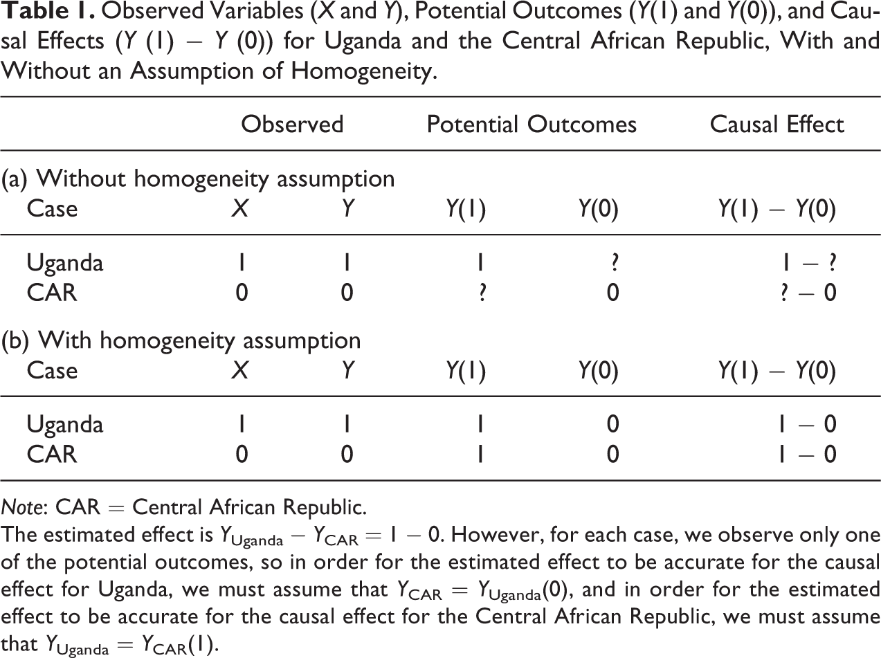
Note: CAR = Central African Republic.

The estimated effect is Y _Uganda − Y _CAR = 1 − 0. However, for each case, we observe only one of the potential outcomes, so in order for the estimated effect to be accurate for the causal effect for Uganda, we must assume that Y _CAR = Y _Uganda(0), and in order for the estimated effect to be accurate for the causal effect for the Central African Republic, we must assume that Y _Uganda = Y _CAR(1).

However, if we assume that Uganda and the CAR are similar enough on values of the control/matching variables (M ₁ and M ₂) to be homogenous, then the observed Y value for Uganda serves as a proxy for the counterfactual Y value for if the CAR had X = 1 (Y _Uganda = Y _CAR(1)). Similarly, the observed Y value for the CAR serves as a proxy for the counterfactual Y value for if Uganda had X = 0 (Y _CAR = Y _Uganda(0)). This homogeneity assumption implies that the estimate of Y _Uganda − Y _CAR = 1 − 0 equals the effect of British colonial history for both Uganda (Y _Uganda(1) − Y _Uganda(0)) and the CAR (Y _CAR(1) − Y _CAR(0)).

“Most Similar” Contrasting Case

Many applications of the comparative method do not begin with the selection of the most similar pair of cases with differing values of the explanatory variable. Researchers often start with a case of interest and generate a theory about that case with an intensive within-case study. The theory is tested using within-case information that was not used for theory generation and is then further tested by selecting a contrasting case. What additional leverage does a contrasting case bring to this type of analysis?

In order for the comparative method with a most similar contrasting case to be valid and for the contrasting case to provide leverage, we must assume homogeneity of the potential outcomes, like for the comparative method with the most similar pair. ¹² Even though these studies are often labeled “most similar” design, a most similar contrasting case may not be the most similar or perhaps not even very similar to the case of interest, and there are likely to be other cases that are more similar to one another on the control variables and have the same value of the independent variable. If such additional cases are available, placebo tests as in the stylized example in the previous sections can help assess this homogeneity assumption and extent of the leverage provided by the contrasting case.

We demonstrate this with Epstein (1964), which assesses the argument that the “uncohesive and nonresponsible character of American parties” (Y _US = 0) is due to the separation-of-powers system of government (X _US = 0). This argument has been made with a comparison to Britain with its parliamentary system (X _Br = 1) and cohesive parties (Y _Br = 1), but Epstein uses Canada as a contrasting case to the United States. Using Epstein’s control/matching variables, we show that while Canada is likely the most similar case to the United States, Britain and perhaps Australia are more similar to Canada than Canada is to the United States. We further show how our confidence in Epstein’s argument is strengthened by the inferential leverage provided by these additional units.

Epstein (1964) begins by discussing the similarity between the United States and Canada: Both are socially and culturally diverse; cover large land areas; are federal systems in which the states or provinces have substantial powers; have similar social and economic class structures; and have single-member, simple plurality election systems (Epstein 1964:46-48). By comparing the United States to Canada, which has a British-style parliamentary system with an executive responsible to a popularly elected legislature (X _Can = 1) (p. 48) and cohesive legislative parties (Y _Can = 1) (p. 52), Epstein concludes that the system of government has an effect on the cohesiveness of political parties (Y _Can (1) − Y _US (0) = 1 − 0 = 1). These variables are summarized in Table 2.

OPEN IN VIEWER

Table 2.

Variables in Epstein (1964) Study.

	United States		Canada		Britain
Y: Cohesiveness of political parties	Low		High		High
T: System of government	Separation of powers		Parliamentary		Parliamentary
M 1: Social and cultural diversity	African Americans and slavery legacy	∼∼	Francophones in Quebec	∼	Scots, Welsh in home regions
M 2: Land area	Large	∼	Large	∼∼	Small
M 3: Federal	Federal	∼	Federal	∼∼	Unitary
M 4: Class structure	Democracy before industrialization	∼	Democracy before industrialization	∼∼	Past feudalism, industrialization first
M 5: Electoral system	SMD, plurality	∼	SMD, plurality	∼	SMD, plurality

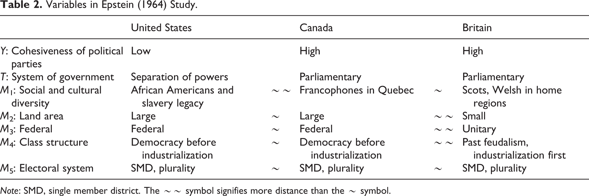
Note: SMD, single member district. The ∼∼ symbol signifies more distance than the ∼ symbol.

Although Epstein is commendably explicit in listing his control/matching variables, he does not comment on the weight that should be assigned to each control/matching variable. Such weights are unnecessary for his argument that Canada represents a better match for the United States than Britain does for the United States if the United States is more similar to Canada than to Britain on all of the control/matching variables. But they are necessary for checking the homogeneity assumption. Even if Canada is closer to the United States than is Britain, the Canada/Britain comparison would provide a placebo test for the Canada/U.S. comparison if, as depicted in Figure 2, Canada is as close or closer to Britain than it is to the United States. ¹³ Canada may be closer to Britain overall even if it is more similar only on one of the control/matching variables, if this variable is weighted sufficiently highly.

OPEN IN VIEWER

Figure 2.

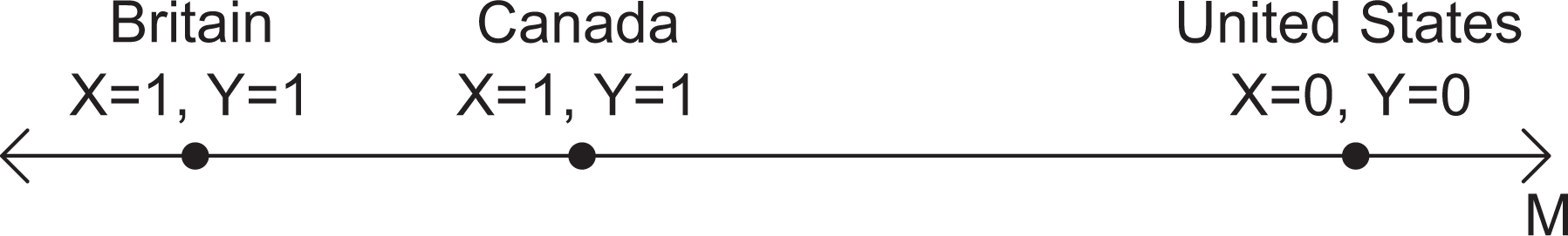
Example of “Most Similar” Contrasting Case Design, Epstein (1964). Epstein’s matching variables are weighted such that Canada is more similar than Britain to the United States and is more similar to Britain than to the United States.

Social and cultural diversity (M ₁ in Table 2) is one variable on which Canada is arguably more similar to Britain than to the United States. Epstein (1964) likens the presence of the Francophone minority population in Canada to the African American population in the United States and describes it a “divisive force” (p. 47), but the Francophones’ position in Canadian politics and society appears closer to that of the Scottish and Welsh populations in Britain. In both Britain and Canada, these minority populations are linguistically and culturally distinct from the majority population and still dominate today in areas they occupied prior to the arrival of the majority population. Moreover, these minority populations in Britain and Canada do not have the legacy of being enslaved by the majority population.

If this control/matching variable were weighted sufficiently heavily, Canada would still be more similar to the United States than is Britain, but more similar to Britain than to the United States. With this weighting, the comparison of Britain and Canada provides a placebo test, since they must be causally homogeneous if the United States and Britain, which are less similar to each other, are assumed to be causally homogeneous. Because Britain and Canada have the same value of the explanatory variable (parliamentary system, X = 1) and the same value of the outcome variable (cohesive legislative parties, Y = 1), causal homogeneity between Britain and Canada is not invalidated. Consequently, Epstein (1964)’s implicit assumption that Canada and the United States are causally homogeneous is also not invalidated, bolstering our confidence in his argument.

This example highlights the importance of making explicit the list, measurement, scaling, and weighting of the control/matching variables. Even though Canada appears to be the case that is most similar to the United States on each of these variables, it may be that Canada is more similar to Britain or another country depending on how those control/matching variables are weighted for an overall assessment of similarity. Indeed, Canada may also be more similar to Australia than to the United States, so that the Australia/Canada comparison may also be a placebo test for Epstein’s argument for the United States. ¹⁴ But to make such a claim and conduct a placebo test, as we did using Britain, it is necessary for the list, measurement, scaling, and weighting of the control/matching variables to be clearly specified. It is not possible to gain inferential leverage from additional units without this information. ¹⁵

The existence of these placebo tests implies that a rigorous approach to the comparative method must consider the similarity between many more pairs of units than are implied by Lijphart (1975). The most direct way to accomplish this is to provide a method for assessing similarity that can be replicated by other researchers, and the “list, measure, scale, and weight” standard we discuss here and is implied by large-n matching procedures is one option. ¹⁶ In the next section, we demonstrate that when this standard is not satisfied, it is impossible to assess the inferential leverage provided by the contrasting case.

“Sufficiently Similar” Contrasting Case

While the Epstein (1964) study is a straightforward example of the comparative method for theory testing, it is often difficult to tell whether small-n comparative studies use comparisons for theory generation, theory testing, or both. For example, Moore (1966) uses numerous comparisons in Social Origins of Dictatorship and Democracy in presenting his argument for how the landed upper classes and the peasantry affected the development of modern democratic, communist, and fascist regimes by the mid-twentieth century. He justifies his use of comparisons by writing that “a comparative perspective can lead to asking very useful and sometimes new questions. There are further advantages. Comparisons can serve as a rough negative check on accepted historical explanations” (p. xix). Moreover, Skocpol and Somers (1980) characterize Moore’s use of comparative history as “primarily for the purpose of making causal inferences about macro-level structures and processes” (p. 181) and present his use of “negative cases” as an application of Mill’s method of difference (p. 183).

As discussed in the fourth section, Mill’s method of difference requires a number of assumptions beyond homogeneity for simultaneous theory generation and theory testing. If homogeneity does not hold, then neither the comparative method nor Mill’s method of difference will produce a meaningful conclusion.

We consider Moore’s use of Japan as a contrasting case to China and, for illustrative purposes, proceed as if the comparative method were being used for theory testing. But, as we will elaborate, Japan may not be the most similar contrasting case for China. Since Moore makes no explicit claims to this effect, his implicit argument is that Japan is a “sufficiently similar” contrasting case for China. It is rare in practice to be able to make the case that a contrasting case is “most similar” as in Epstein (1964), since evaluating the control/matching variables for all possible contrasting cases is usually prohibitively costly and requires expertise in many areas. Researchers are often only able to examine a subset of cases and/or variables, so that implicit arguments that the cases being compared are “sufficiently similar” are quite common.

In Moore’s use of Japan as a contrasting case to China, the fundamental question is: To what extent should the comparison with Japan increase our confidence in Moore’s argument about China? Unfortunately, we are unable to definitively answer this question, because Moore does not provide the road map that would be necessary to determine (1) whether there are any more similar contrasting cases that would produce a different conclusion or (2) whether there are any more similar pairs with the same value of the independent variable that could function as placebo tests.

The major difficulty is that Moore (1966) does not clearly list all of his explanatory variables or distinguish between his independent variables and his control/matching variables. Nor are guidelines provided for how the variables should be measured or how the control/matching variables should be scaled or weighted for an overall assessment of similarity between these cases. For this analysis, we rely and build upon Skocpol (1973)’s distillation of three “explanatory variable clusters” from Social Origins. We also infer how the variables should be measured for other possible cases and incorporate our own ideas on how the variables might be scaled and weighted in establishing overall similarity from our reading of Moore.

With the variables from Skocpol (1973) and our delineation of independent and control/matching variables, we argue subsequently that Korea (then Choson) is more similar to China than is Japan to China and show that Korea provides inferential leverage by casting doubt on the validity of Moore’s China/Japan comparison. We further demonstrate that Korea need not be more similar to China than is Japan to invalidate this comparison, by considering foreign threats in the nineteenth century as an additional control/matching variable. The overall conclusion is that Moore’s contrast with Japan adds little confidence to his argument for China beyond his case study of China.

Similarity With Moore’s Variables

Following several case studies, Moore describes his complex argument for the emergence of democratic, fascist, and communist regimes in three thematic chapters in Part III of Social Origins. In a critical review of this work, Skocpol (1973) organizes Moore’s overall argument into three explanatory variable clusters—bourgeois impulse, mode of commercial agriculture, and peasant revolutionary potential. Her summary of Moore’s coding of the cases on these variables is partially reproduced in Table 3. These three factors shape which classes ally with each other as the economy begins to modernize, whether there is a peasant revolution, and ultimately what type of modern regime emerges.

OPEN IN VIEWER

Table 3.

Summary of Moore (1966), Based Upon Skocpol (1973), Including Our Own Coding of Choson/Korea.

	Japan	Korea/Choson	China
Y: Communist regime	No (0)	Partial (0/1)	Yes (1)
T: Peasant revolutionary potential	Low (0)	Low (0)	High (1)
M 1: Bourgeois impulse	Medium	Moderately weak	Weak
M 2: Mode of commercial agriculture	Labor repressive	Labor repressive	Labor repressive

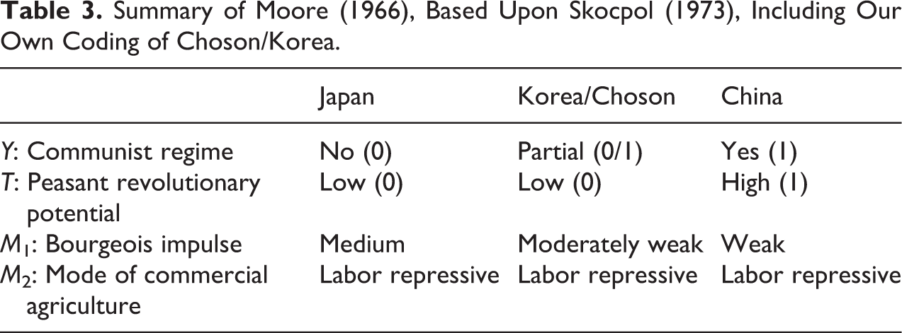
To apply the comparative method to Moore’s China case study and its contrast with Japan, we must first define and separate the three explanatory variable clusters into independent variables and control/matching variables. As coded by Skocpol (1973), mode of commercial agriculture is certainly one of the control/matching variables, because both China and Japan are coded as labor repressive. Peasant revolutionary potential is certainly one of the independent variables because China is coded as high while Japan is coded as low. It is less clear whether bourgeois impulse, for which China is coded as weak while Japan is coded as medium strength, is a secondary independent variable or a control/matching variable on which the two cases are not perfectly matched.

We treat bourgeois impulse as a control/matching variable for two reasons. First, it is difficult to distinguish between bourgeois impulse and mode of commercial agriculture or determine how to measure them. The mode of commercial agriculture generally refers to whether the upper classes rely on the market or use “political” and more traditional social means to supply labor to work its land holdings (Moore 1966:433). Skocpol (1973:13) relies on “scattered remarks” to figure out how to measure the strength of bourgeois impulse and “wonder[s] if these implicit criteria were applied independently of results, or consistently.” We were similarly uncertain of Moore’s definition of bourgeois impulse, although we determine that the strength of bourgeois impulse is associated with the growth of cities, the rise of an urban commercial and manufacturing class, and demand from commodity markets. We are also uncertain about when to measure these variables, which is problematic because these features of a country’s political economy and society can be very different over the long run.

Both bourgeois impulse and mode of commercial agriculture are rooted in the relationship between the state, the landed upper class, and the overall socioeconomic and political system, and consequently, these variables are hard to disentangle. In China, for example, upper-class families would invest in a son’s Confucian education for him to sit for exams to join the imperial bureaucracy, with the understanding that this investment would be “recouped” through the land and wealth to be acquired through his appointment (Moore 1966:165). When growing commerce threatened the economic and social status of this scholar–landlord class, the imperial bureaucracy generally tried to “absorb and control commercial elements” (p. 175) through taxation and the establishment of monopolies. The availability of this route to wealth through the state “deflected ambitious individuals away from commerce” (p. 174), contributing to the weakness of bourgeois impulse. Moreover, the “labor-repressive” mode of commercial agriculture, or “political methods…[that kept] the peasants at work” (p. 180) were a crucial part of “making property pay” (p. 181), ¹⁷ both attracting and supporting the landed upper class.

Second, Moore emphasizes peasant revolutionary potential when accounting for why no peasant revolution took place and consequently no communist regime emerged in Japan (pp. 254-55). This peasant revolutionary potential is theoretically more distinct from bourgeois impulse and mode of commercial agriculture. While the latter two clusters mostly concern the relationship between the landed upper classes and the state, peasant revolutionary potential focuses on the relationship between the landed upper classes and the peasants, whose roles in the peasant revolution leading to communism Moore seeks to understand (p. xxiii). Moore (1966:478) defines peasant revolutionary potential as “the weakness of the institutional links binding peasant society to the upper classes, together with the exploitative character of this relationship,” but provides few guidelines for its measurement.

Having designated the independent and control/matching variables in this way, we can consider the Japan/China comparison. We denote peasant revolutionary potential as X and whether there is a communist regime as Y using notation from the previous sections. With Skocpol (1973)’s coding of peasant revolutionary potential as either high (X = 1) or low (X = 0), China can be characterized as X _C = 1, while Japan can be characterized as X _J = 0. The logic of the comparison here is that, despite not being perfectly matched on the control/matching variables, Japan is “sufficiently similar” to stand in for China with low peasant revolutionary potential. Korea (then Choson) may provide evidence against the sufficiency of this similarity. As in China, the monarchy and the landed upper class (yangban) in Korea relied heavily on tenant farmers for income and tax revenues (Shin 1998). The landed upper class acquired and maintained its land holdings through having family members qualify for state administrative positions through examinations on Confucian scholarship as in China. Moreover, the “Yi Dynasty (1392–1910) consciously tried to form its administration according to a neo-Confucian interpretation of ancient Chinese works and had more continual and stronger Chinese influence on the shape of the state than did Japan” (Sorensen 1984:306). ¹⁸ The overall relationship of the landed upper classes to the state in Korea was more like that of the scholar–landlords in China than that of the nonlanded warrior aristocracy to the centralized feudal state in Japan. Therefore, although we do not have a good understanding of the coding of bourgeois impulse, we assign Korea a value of moderately weak in contrast to Japan’s value of medium. This assessment of the similarity of the cases is depicted in Figure 3. ¹⁹

OPEN IN VIEWER

Figure 3.

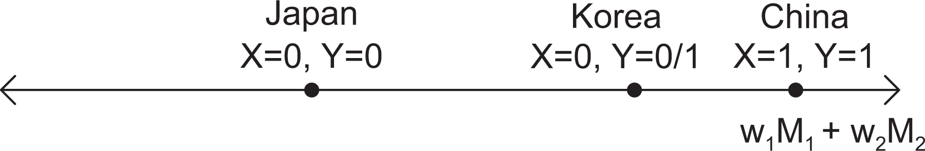
Example of “Sufficiently Similar” Contrasting Case Design, Moore (1966). Skocpol’s summary of Moore’s control/matching variables is weighted such that Korea is more similar to China than is Japan. The case of interest for this study is China.

However, despite the similarities between China and Korea on the control/matching variables, Korea appears to be more similar to Japan on the independent variable, peasant revolutionary potential. In China, peasant revolutionary potential is high (X _C = 1) because “[t]he government and the upper classes performed no function that the peasants regarded as essential for their way of life” (Moore 1966: 205). Institutional links between peasant society and the landed upper classes were too weak to absorb the pressures from its exploitative nature (p. 478). At the same time, “solidary arrangements…constitute[d] focal points for the creation of a distinct peasant society in opposition to the dominant class and [served] as the basis for popular conceptions of justice and injustice that clash[ed] with those of the rulers” (p. 479).

In Japan, peasant revolutionary potential is low (X _J = 0) because there was a “close link between the peasant community and the feudal overlord, and his historical successor the landlord” (p. 254). Moore reports that the gentry provided some relief in times of poor harvests and that “the Japanese peasant community provided a strong system of social control that incorporated those with actual and potential grievances into the status quo” (p. 254). Moreover, irrigation and rice planting required cooperation among villagers (pp. 263-64), and the tax system created the “tightly knit character of the Japanese village…[which] tied the peasants closely to their rulers” (pp. 258-59).

In Korea, peasant revolutionary potential is also low (X_K  = 0) because village organization connected landlords and tenants and funneled tenant grievances through established channels. Rural Korean society had various institutions led by the rural elite such as village compacts (tongyak), credit rotating systems (kye), labor reciprocating systems (pumashi), and lineage associations (munjung). The rural elite also “maintained close ties with [the cultivators] because they…[lived] in the countryside with other economically less fortunate residents” (Kim 2007:997). The Yi dynasty had a system of village organization like the Chinese pao-chia, but they emphasized the subvillage neighborhood unit rather than the larger village unit. Their responsibilities were more limited, so that they “counterbalance[d] whatever strength the villages might have developed” (Eikemeier 1976:108).

Since Korea is more similar on the control/matching variables to China and has the same value of the independent variable as Japan, it appears to be a more similar contrasting case to China than is Japan. We code the outcome variable for Korea as Y _K = 0/. But without clear guidance from Moore on when this variable should be measured, it is difficult to code the outcome variable since Korea becomes communist only in its northern half in the second half of the twentieth century. Even though Moore’s discussion of China’s peasant revolution only extends to the 1930s, this coding for Korea for after the Korean War (1950–1953) is compatible with the time period used by Moore to code China as communist (Y _C = 1), since the Chinese Communists did not consolidate their control over the country until the Nationalists were driven from the mainland in 1949. This is also consistent with a coding of the outcome in Japan as not communist (Y _J = 0), although it is inconsistent with Moore’s coding of the outcome in Japan as fascism, since by 1949 the fascist regime in Japan had been defeated and replaced by American military occupation. Japan’s industrialization and modernization through a “revolution from above” also began decades earlier. However, it is clear that when restricting the analysis to the variable clusters presented in Skocpol (1973), comparing China (Y _C = 1) with Korea (Y _K = 0/1) leads to a less certain conclusion about the effect of peasant revolutionary potential than does comparing China with Japan (Y _J = 0).

Similarity Including Foreign Threat

Our assessment of similarity between the cases and hence the inferences drawn on the basis of similarity may change if we consider additional control/matching variables. This section considers one such additional factor: the extent of foreign threat in the nineteenth century (labeled M ₃). ²⁰ China, Japan, and Korea all faced threats from foreign powers that triggered major social and political changes. The First Opium War (1839–1842) made clear to the Qing dynasty the backwardness of the Chinese military, and Chinese losses led to the recognition of extraterritoriality and the transfer of Hong Kong to the British Empire. The arrival of American ships on Japanese shores in 1853 forcefully ended Japan’s isolationist foreign policy and was the start of unwanted engagement with several western powers demanding the opening up of trade. Similarly, Korea had cut off almost all international relations as the “hermit kingdom” until the 1860s when the Russians, French, British, Americans, and Japanese opened up trade and established extraterritoriality through military invasions and gunboat diplomacy. On this control/matching variable, Korea is more like Japan than China in that these foreign threats were sudden, major disruptions to centuries of isolation. By contrast, China had been the predominant power in East Asia with active military campaigns to extend its empire and tributary state system. If we rank the three countries on this variable, we would find China with the lowest foreign threat, Japan with moderately high foreign threat, and Korea with high foreign threat.

Figure 4 presents the matching space, with Moore’s control/matching variables (w ₁ M ₁ + w ₂ M ₂) on the x-axis, as in Figure 3. We have not explicitly chosen the weights w ₁ and w ₂, because all three countries are coded the same on M ₂ (labor-repressive mode of commercial agriculture) and consequently the weights do not affect the scaling on the x-axis. ²¹ Japan, Korea, and China keep the same location on the x-axis in Figures 4 from Figure 3, but differ in the extent of nineteenth-century foreign threat (M ₃) which is represented on the y-axis. With just our ordinal rankings of the countries on w ₁ M ₁ + w ₂ M ₂ and M ₃, we can only speculate as to the exact locations of the three countries in Figure 4. Our guesses place Japan closer to China than Korea is to China in the matching space, so that Japan is a better match for China than is Korea. This can be seen in Figure 4, with Japan lying on the dotted arc centered at China while Korea lies beyond it. It also places Korea closer to Japan than Japan is to China, as shown by Korea’s positioning inside the dashed arc centered at Japan and passing through China.

OPEN IN VIEWER

Figure 4.

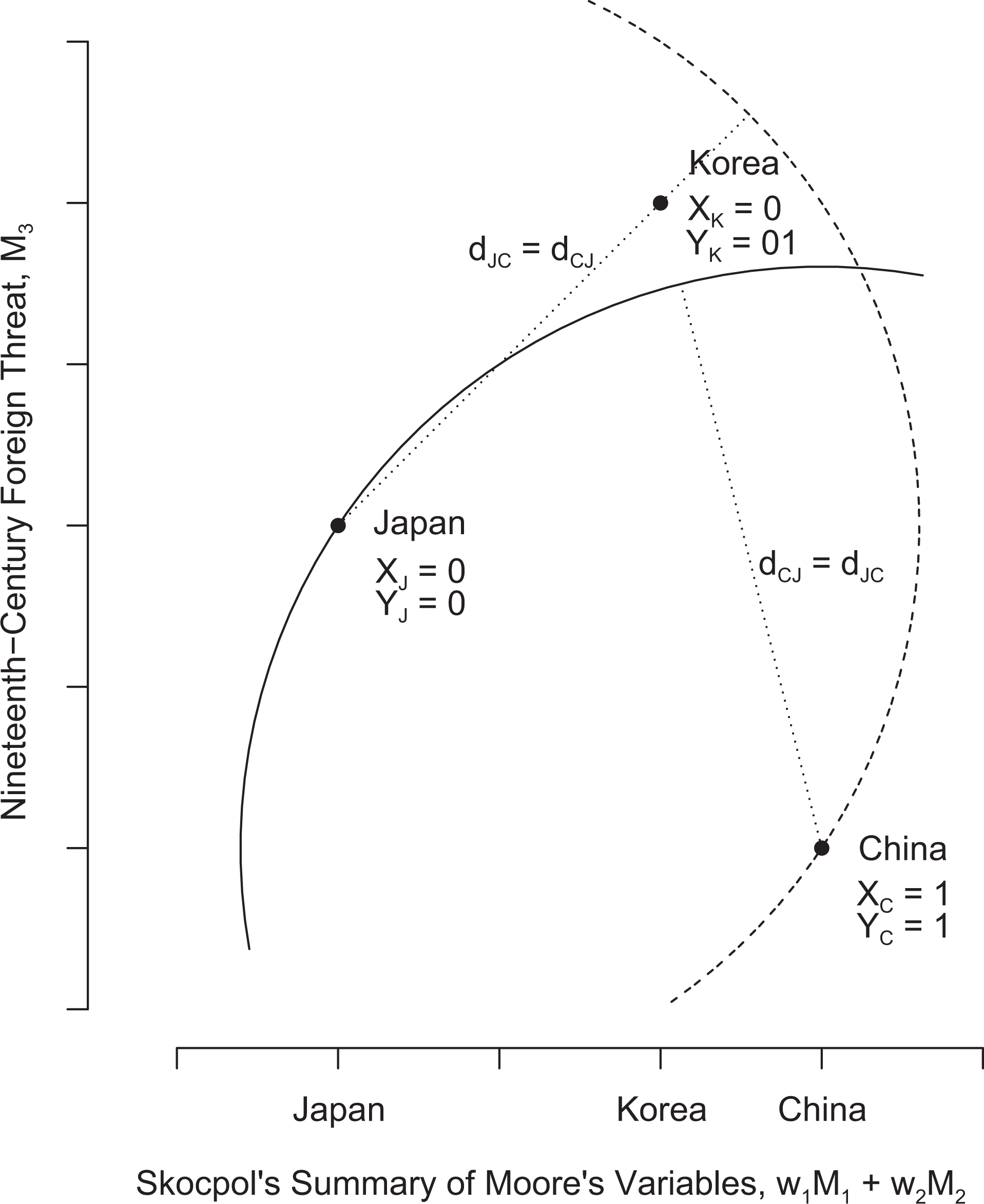
Moore (1966), with nineteenth-century foreign threat on the y-axis. The arcs and radii allow the comparison of distances between the points. These show that Korea is further away from China than is Japan, and it is closer to Japan than is China. Therefore, the Japan/Korea comparison can be used as a placebo test for the China/Japan comparison.

Even though Japan is more similar to China than is Korea in this arrangement, the Korea/Japan comparison still provides inferential leverage and casts doubt on the homogeneity assumption required for the China/Japan comparison. Korea and Japan, which are more similar than are China and Japan and have the same value of the independent variable X, do not have the same outcome Y. From this failed placebo test, we would conclude that Japan is likely not sufficiently similar to China for a meaningful comparison and that the contrast with Japan adds little to our confidence in Moore’s argument for China.

This example highlights that without a clear road map from Moore, we cannot determine what placebo tests are possible or the extent to which the comparison with Japan should increase our confidence in Moore’s argument about China. The analysis required us to make a number of assumptions about how to measure the dependent variable, what was the independent variable, what control variables should be included, how they should be measured and scaled, and what relative weights should be accorded them. The locations of the cases in Figure 4 reflect our assumptions, which allowed us to use Korea to evaluate whether Japan/China is a meaningful comparison.

Conclusion

Increasing the number of observations is often recommended to address limitations to small-n studies that use the comparative method for causal inference (King et al. 1994:208; Lijphart 1975:163). However, this is an impracticable or undesirable solution in some circumstances. One such circumstance is when there is only one pair of cases with X = 1 and X = 0 that are similar on the control/matching variables, as in the stylized example of landlocked African countries. Increasing the number of pairs with differing values of the independent variable would only have reduced the validity of this analysis. Another is when we seek causal effects for individual cases, as for the United States in Epstein (1964) or for China in Moore (1966). Without additional assumptions, increasing the number of pairs with differing values of the independent variable would provide more leverage only for average causal effects and not for case-specific causal effects.

By clarifying the assumptions necessary for the comparative method, we showed that even in these situations, placebo tests may be available such that units beyond those under comparison can add inferential leverage to the analysis. Lesotho and Zambia, a pair of former British colonies, cast doubt on inference from the Uganda/CAR comparison in our stylized example. The explicit comparison of Britain with Canada conferred greater confidence in the conclusions drawn from the comparison of the United States and Canada by Epstein (1964). Finally, the comparison of countries with low peasant revolutionary potential, Korea and Japan, made us reconsider Moore’s use of Japan as a contrast to China.

As noted previously, these placebo tests point to a previously unrecognized way in which scholars of comparative politics with regional or area expertise can contribute to the broader discipline. Such experts frequently offer proximity to causal mechanisms, better measurement, and sensitivity to the question of whether a general theory applies in particular contexts. But such scholars may also utilize their expertise in evaluating the validity of small-n comparisons that do not include a case from their own region, if similarity should be judged the same way in their own region as in a given study. That is, an Africanist might point out that the similarity argument being made to justify the comparison of two Latin American countries would imply that two sub-Saharan African countries that are at least as similar should have the same outcome—but perhaps do not. Such observations by a specialist on sub-Saharan Africa that falsify homogeneity would be useful even if the scope of inference of a given study is limited to these two Latin American countries. The Latin America specialist might argue that similarity should be judged differently in sub-Saharan Africa, but this argument would need to be made explicitly.

The possibility of these tests also enjoins researchers to take two steps beyond the current practice for small-n studies of specifying the control/matching variables that justify the selection of the cases to be compared. First, they require that the dependent, independent, and control variables be clearly defined and delineated before the analysis and that researchers provide enough information such that these variables can be measured on additional units. Second, they require that researchers explicitly state how the control/matching variables are weighted in making a claim of similarity. If these steps are too onerous, then the comparison case adds little inferential value and should not be included in the study. In other words, the study should focus on establishing the causal effect for the main case through other techniques and not include a second case just to be comparative. But wherever possible, researchers using the comparative method should follow these steps to allow others to conduct placebo tests to build on their analyses. These steps will ultimately improve the credibility of conclusions drawn from small-n comparative studies.