A Careful Look at Modern Case Selection Methods

Abstract

Case studies appear prominently in political science, sociology, and other social science fields. A scholar employing a case study research design in an effort to estimate causal effects must confront the question, how should cases be selected for analysis? This question is important because the results derived from a case study research program ultimately and unavoidably rely on the criteria used to select the cases. While the matter of case selection is at the forefront of research on case study design, an analytical framework that can address it in a comprehensive way has yet to be produced. We develop such a framework and use it to evaluate nine common case selection methods. Our simulation-based results show that the methods of simple random sampling, influential case selection, and diverse case selection generally outperform other common methods. And, when a research design mandates that only a very small number of cases, say one or two, be selected in the course of a research program, the very simple method of sampling from the largest cell of a 2 × 2 table is competitive with other, more complicated, case selection methods. We show as well that a number of common case selection strategies work well only in idiosyncratic situations, and we argue that these methods should be abandoned in favor of the more powerful and robust case selection methods that our analytical framework identifies.

Keywords

case study research design causal inference random sampling small-n studies

Introduction

Case study analysis is one of the more prominent research methods in empirical social science. One can readily find case studies in areas dominated by qualitative modes of inquiry, and within political science case studies are relatively common in the fields of comparative politics and international relations. A simple JSTOR¹ search (on December 6, 2012) for the terms “case study,” “case-study,” “case studies,” or “case-studies” in the full text of articles in the American Political Science Review (APSR) from 1998 to 2007 returns 108 results. Similar JSTOR searches for other methodological terms yield the following: “regression,” 210 hits; “probit,” 84 hits; “instrumental variables” or “instrumental variable,” 33 hits; “field experiment,” eight hits. Nearly 11 APSR articles per year make some mention of case studies, and this is a larger number than that for all the other terms above save “regression.”

Performing a similar analysis on the holdings of a journal that specializes in comparative and international politics suggests an even greater role for the case study method. A JSTOR search (on December 6, 2012) for the terms “case study,” “case-study,” “case studies,” or “case-studies” in the full text of articles in World Politics from 1997 to 2006 returns 64 results. Similar JSTOR searches for other methodological terms yield the following: “regression,” 70 hits; “probit,” 17 hits; “instrumental variables” or “instrumental variable,” nine hits; “field experiment,” three hits. The point to take from this is that case study methods are commonly used in political science, particular among scholars of comparative and international politics.

A key question—arguably the key question—faced by scholars pursuing case studies is that pertaining to case selection criteria. Namely, a scholar carrying out a case study must confront the question, what criteria should he or she use to choose his or her case or a set of cases for analysis? Should, for example, a case for analysis be picked on the basis of being representative of a large set of possible cases? Or, should a case be chosen because it is distinctly nonrepresentative? Relatedly, should a case study researcher use deterministic rules to select cases—by, say, choosing cases that are guaranteed to be different along some notable dimensions—or should case selection include a stochastic element?

Decisions regarding case selection rules must be made early on in a research program, and these decisions can have a profound effect on the ultimate quality of said program. Indeed, the conclusions of a case study analysis are, by construction, valid only to the extent that the case or cases used to support them are chosen in a compelling way, compelling suitably defined.

How might one know if the criteria for case selection employed in a case study research program are adequate or effective and what precisely might such a characterization mean? Different researchers employ case study analysis to achieve different goals,² and as such, the efficacy of any particular rule for case selection must be evaluated in terms of its ability to achieve a particular research objective. The specific research goal that we consider in this article is inference about the effects of causes. By inference, we mean the use of data from a fixed number of cases to make claims about a larger set of cases. We use the terminology effects of causes in the manner of Holland (1986). Holland makes a useful analytic distinction between questions about effects of causes and questions about causes of effects. The former questions take forms similar to, “What is the effect of enrollment in a particular test prep course (relative to no test prep) on SAT scores?” The latter questions take forms similar to “Why do some students do better on the SAT than other students?” While both types of questions can be interesting, Holland and others have argued that questions about effects of causes (“What’s the effect of test prep on test scores?”) are narrower and thus easier to answer in a credible way than are questions about causes of effects (“Why do some students do better on the test than others?”). Further, many would argue that methods for producing credible answers to questions about effects of causes are well understood and relatively uncontroversial, whereas methods for producing credible answers to questions about causes of effects are less well developed and more controversial. For these reasons, throughout this article, we focus on inference about the effects of causes.

To assess the efficacy of various case selection methods with respect to this goal, we develop an analytical framework that can be used to evaluate case selection methods, and we then apply the framework to common case selection rules that scholars have historically used to select cases for research. These rules are described by Seawright and Gerring in Chapter 5 of Gerring (2006) ³; see also Seawright and Gerring (2008). We note that methods similar to those considered by Seawright and Gerring have been discussed by other researchers as well. We comment shortly on these methods, but for the moment, it suffices to say that Seawright and Gerring’s exploration of case study methods constitutes a current and comprehensive study of this research methodology, as it appears in empirical political science.

The case selection methods that we explore here are found primarily in qualitative research designs. Such designs typically have small sample sizes, say, ten observations or fewer. Nonetheless, our framework for analysis should not be thought of as a framework that pertains only to qualitative research. Indeed, rather than focusing on “case selection criteria,” we could have chosen to focus instead on “observation selection criteria” or “unit selection criteria.” Nothing would have changed analytically had we relied on the latter terms, but we use the former exclusively because of the prevalence of case studies in small n, qualitative research designs. While at times in what follows we refer explicitly to qualitative research, we note that our findings have little (or one might even say nothing) to do with precisely how a researcher studies a case once it is chosen for analysis. As we will make clear shortly, we do assume that a researcher can formulate particular counterfactual claims about the cases chosen for detailed study, but we are agnostic as to methods by which those claims are generated. Our framework is a general one that can be used to study the effectiveness of selecting some cases (or units) for more extensive, in-depth examination when the goal is to infer the effect of a cause, and we turn to it now.

A Framework for Causal Inference and Case Selection

While much attention has been paid to case study methodology in recent years, there is at present no general mathematical framework for thinking about how case studies can help improve the quality of causal inferences. Similarly, while many practitioners of case study methodology acknowledge a fundamental role for counterfactuals in what they do (see inter alia Fearon 1991; Ferguson 1999; Hawthorn 1993; Lebow 2000; Levy 2008), these same researchers have not attempted to place their methodologies within an explicitly counterfactual causal model such as proposed by Neyman, with Iwaszkiewicz, and Kolodziejczyk (1935), Rubin (1974, 1978), Robins (1986), and Pearl (1995, 2000; but see Sekhon 2004). We attempt to bridge these gaps, and the remainder of this section details our attempt to place case study research within an explicitly counterfactual causal framework. The benefit of this approach is that—to the extent that our account of case study research is persuasive—case selection methods can be evaluated according to standard statistical criteria such as bias, root mean square error (RMSE), and variance reduction, at least with respect to our stated research goal of inferring effects of causes. Without reference to standard measures like these, it is difficult if not impossible to evaluate whether a given case election technique “works.”

The Basics

Consider the situation where a researcher observes the value of a dichotomous causal variable along with the value of a dichotomous outcome variable for each unit in a sample from some well-defined population. By “causal variable,” we mean here a variable that could plausibly be a cause of the outcome in question. Some readers may find it more convenient to think of what we are calling a causal variable as a “treatment variable.”

We let i = 1,…N index sample units, $X_{i} \in \{0, 1\}$ denote the causal variable for unit i, and $Y_{i} \in \{0, 1\}$ denote the observed outcome from unit i. Throughout the article, we will refer to units for which X_i = 1 as “treated units,” units for which X_i = 0 as “control units,” units for which Y_i = 1 as “successful units,” and units for which Y_i = 0 as “unsuccessful units.” Such experimental terminology is merely a convention that we will use here. We assume that (X_i , Y_i ) for i = 1,…N are independent replicates drawn from some joint distribution P_XY . Finally, we use the notation x_i and y_i to denote individual realizations of X_i and Y_i and x and y to denote the N vectors of these realized values.

To fix ideas and make our notation concrete, we introduce data from Licklider (1995) on method of civil war termination and war resumption (see Table 1). The causal question of interest implicit in this table is whether negotiated settlements (X = 1) decrease the likelihood of war resumption (Y = 0) relative to what occurs when military victory ends a war (X = 0).⁴

Table 1.

Relationship Between Method of Civil War Termination and War After Termination Among “Identity Civil Wars.”

	Y = 0	Y = 1
	Same war resumes after termination	No war after termination
X = 0
Termination is military victory	5	19
X = 1
Termination is negotiated settlement	6	3

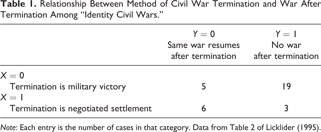
Note: Each entry is the number of cases in that category. Data from Table 2 of Licklider (1995).

Throughout this article, we assume that it is possible for a researcher to sample units from the population of interest (or to collect data from the entire population of interest) and classify the selected units on the basis of their values of the causal variable X_i and outcome variable Y_i of interest. In other words, we assume that a researcher in her research program of interest can construct a 2 × 2 table similar to Table 1.

Even with a table akin to Table 1, one cannot directly identify causal effects. Simply put, this is because of the possibility of confounding bias or what is often called omitted variable bias. For example, one might observe in a 2 × 2 table of X_i and Y_i that when X_i =1, one tends to also see that Y_i = 1. One cannot conclude from this that a unit’s treatment status, that is, X_i = 1, leads to success, that is Y_i = 1, because a third—and unobserved—variable might be a cause of both X_i and Y_i .

We adopt the notation Y_i (X_i = 0) and Y_i (X_i = 1) to denote the value of unit is outcome variable if X_i is set equal to 0 and 1, respectively, by an outside intervention that leaves all preintervention variables unchanged. Y_i (X_i = 0) and Y_i (X_i = 1) are referred to as potential outcomes, or, in some cases, counterfactual outcomes, and we write $Pr (Y (X = x) = y)$ to express the probability that the outcome variable from a randomly chosen unit will take value y when the unit in question is assigned X = x. Causal quantities such as the average treatment effect (ATE):

A T E = Pr (Y (X = 1) = 1) - Pr (Y (X = 0) = 1)

can be written in terms of the above probabilities.⁵ Note that $Pr (Y (X = x) = y)$ will typically not equal the conditional probability of Y, given X, that is, $Pr (Y = y | X = x)$ . While the latter can be consistently estimated from observed data without additional assumptions, the former cannot—this is the problem of possible confounding bias.

The assumptions typically employed to estimate $Pr (Y (X = x) = y)$ from observed data are as follows:

$Y (X = 0) ㅛ X | U$ and $Y (X = 1) ㅛ X | U$ for some (possibly high dimensional) set of variables U. Put simply, cases (or units) that have the same value of U look as if their values of X (the causal variable of interest) were randomly assigned. Thus, it is possible to remove confounding bias by adjusting for U.

Y_i (X_i = 0) and Y_i (X_i = 1) do not depend on the realized values of any variables in units other than unit i.

Y_i (X_i = x) = y_i if X_i = x. In words, the observed outcome for case i takes the same value as the potential outcome under the scenario, where the causal variable is set equal to its observed value by outside intervention. The implication is that we get to observe the value of the potential outcome Y_i (X_i = x) when the observed value of X_i is x.

The first assumption is commonly referred to as conditional ignorability of treatment assignment, no unmeasured confounding, and/or selection on observables. The latter two assumptions make up what is commonly referred to as the stable unit treatment value assumption (SUTVA). These assumptions, or close cousins thereof, are the starting point for nearly all principled attempts to infer causal effects from observed data, including analyses based on regression, matching, and inverse propensity score weighting. Our analysis in this article is no exception.

In typical applications, one attempts to define U, so that assumption (1) holds and (a) all variables in U are observable and (b) the number of variables in U is not too large. The reason for this is that the researcher in such a typical application wants to directly adjust for the variables in U by including them in his or her regression model, propensity score model, and so on. We do not pursue this course of action in this article. Instead, we think of U purely in conceptual terms as a set of variables that, if known, would perfectly predict the values of the potential outcomes, Y_i (X_i = 0) and Y_i (X_i = 1), for all cases.⁶

Conceiving of U this way allows one to partition U into four equivalence classes that preserve all the information in U relevant for causal inference about the effect of a binary X on a binary Y. Following Chickering and Pearl (1997), Quinn (2008) shows how this can be done for 2 × 2 and 2 × 2 × K tables. We perform the same trick here, using a new categorical variable Z_i to label these four equivalence classes. Table 2 describes Z_i .

Table 2.

Possible Patterns of Potential Outcomes and Coarsest General Confounding Variable.

Y_i (X_i = 0)	Y_i (X_i = 1)	Z_i
0	0	0	Never Succeed
0	1	1	Helped
1	0	2	Hurt
1	1	3	Always Succeed

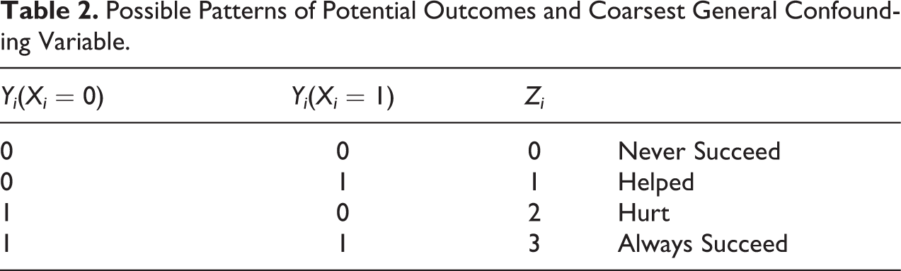
A unit i for which Z_i = 0 has a value of U_i which implies that Y_i will always be equal to 0 regardless of the (possibly counterfactual) value of X_i . We say such a unit is a “never succeeder.” If Z_i = 1, then in contrast, we say that unit i is “helped” by treatment because its potential outcome under X = 1 is equal to 1 (success), while its potential outcome under X = 0 is 0 (failure). If, though, unit i has Z_i = 2, we say that i is “hurt” by treatment because its potential outcome under X = 1 is equal to 0 (failure), while its potential outcome under X = 0 is 1 (success). Finally, if Z_i = 3, then we say that i is an “always succeeder” because its value of U_i is such that Y_i will always equal 1, regardless of the (possibly counterfactual) value of X_i .

To help with intuition, consider the example we invoked earlier regarding the effect of war termination via negotiated settlement on war continuation. Suppose that a qualitative researcher is interested in the case of Paraguay in 1947. Licklider codes this as a case with a military victory and no recurrence of the same war, that is, X_i = 0 and Y_i = 1. After evaluating and weighing the myriad factors which, within the detailed context of the particular case of Paraguay in 1947, contribute both to type of war termination and to continuation of conflict, our hypothetical researcher concludes that this conflict would not have resumed regardless of whether the conflict ended (as it did) in military victory or (as it could have) in a negotiated settlement.⁷ Making a counterfactual claim like this is something that many researchers, particularly historians and scholars of international relations, often do; see Fearon (1991); Hawthorn (1993); Ferguson (1999); Lebow (2000); and Levy (2008). The key piece of intuition that we want to convey at this point is that this counterfactual claim is exactly equivalent to the claim in our terminology that Z_i is known for Paraguay in 1947 and that in fact Z_i is equal to 3 (Paraguay in 1947 is an “always succeeder”). Indeed, any counterfactual claim about the value of the outcome variable in a world where the causal variable X took a different value than its observed value is equivalent to a claim about the value of Z_i for the case in question.

Since Z is defined in terms of the value of the potential outcome pairs, it is clear that conditional ignorability of treatment assignment (assumption 1) holds, given Z. We assume that (X_i , Y_i , Z_i ) for all i are independent replicates from some joint distribution P_XYZ . This means that each case i, which is characterized by treatment X_i , outcome Y_i , and confounder Z_i , is drawn from a common distribution. This is consistent with a scenario where x_i , y_i , and z_i take constant values for each unit i and (x_i , y_i , z_i ) triples are sampled from the population of interest. If P_XYZ were known, then one could write 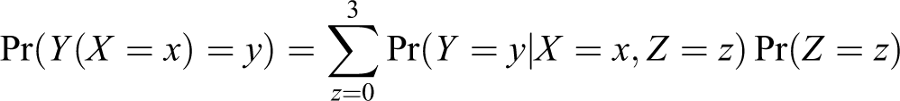$Pr (Y (X = x) = y)$ as:

Pr (Y (X = x) = y) = \sum_{z = 0}^{3} Pr (Y = y | X = x, Z = z) Pr (Z = z)

where the probabilities on the right-hand side of the equation above can be calculated directly from P_XYZ .

Thus, if either U or Z were observed for a sample of units, it would be possible to estimate a variety of causal effects. Quantitative researchers often focus on identifying, measuring, and adjusting for a large collection U of confounders that can be measured for all cases under study. Unfortunately, U (or some subset of variables that are sufficient to control confounding bias) is often difficult to identify and measure. On the other hand, many qualitative researchers often seem more interested in focusing on the particulars of specific cases in the hopes of better understanding the causal mechanisms at work within those cases and whether a particular causal factor played a determinative role in producing the outcome observed for those cases. As noted previously, these sorts of case-specific counterfactual claims are exactly equivalent to claims about the value of Z_i for the case in question. This approach is also not without problems. While some researchers may feel comfortable making claims about the values of Z_i for particular cases, it is fundamentally not possible to know the value of Z_i with certainty for any case because of its counterfactual nature.

In what follows, we let z denote the vector of realized values of Z that are observed by the researcher. Assuming the most optimistic⁸ scenario—that case analysis allows a researcher to accurately determine the realized value of Z_i for an arbitrary unit i—we examine the inferential properties of various methods of choosing cases for detailed examination. Throughout, the assumed goal is the generation of inferences about the effects of causes that extend to cases beyond those chosen for detailed examination.

Case Selection for Causal Effect Estimation

So far we have assumed that (x_i , y_i , z_i ) triples are randomly drawn from a common distribution. The researcher gets to observe (x_i , y_i ) for each i (meaning, treatment, and outcome status for each observation i) but, at least initially, is unable to observe the confounding variable z_i . This gives rise to a two-way table of X and Y that has been effectively marginalized over Z. The aforementioned Table 1 is an example of this.

Nevertheless, the true table of interest for causal inference is the 2 × 2 ×4 table of (X, Y, Z ) values, that is, the table that includes the confounder Z and is not marginalized over it. While it might seem that there is no information in the observed 2 × 2 (X, Y ) table about the unobserved (X, Y, Z ) table of interest, this is not correct. To see why this is the case, note that conditioning on X_i = x_i and Y_i = y_i reduces the set of logically possible values of z_i to two elements. For instance, all of the 19 cases in the (X = 0, Y = 1) cell of Table 1 are either Hurt (Z = 2) or Always Succeed (Z = 3) units. We know this is true because, since Y = 1 in this cell, observations i in this cell cannot be Never Succeed Units or Helped Units, as they would then not have Y_i = 1. We exploit this ability to partially identify the conditional distribution of Z, given X and Y, in what follows.

After this initial sampling of N units has taken place and the (X, Y ) table has been filled out, we allow the researcher to select Q of N initially sampled units for additional inspection. We introduce the variable S_i to indicate whether unit i was selected for additional inspection (S_i = 1) or not (S_i = 0). As noted previously, we are agnostic as to the methods used to study a particular case once it is selected for additional inspection, but we do assume that if case i is selected for additional inspection (S_i = 1), then the value of the confounder Z_i is perfectly observed. This second round of case selection and inspection gives rise to a partially observed 2 × 2 × 4 × 2 table for (X, Y, Z, S).

Let C_xyzs denote the number of cases with X = x, Y = y, Z = z, and S = s. At some points below, we will want to denote cell frequencies that have been summed over some margins of the 2 × 2 × 4 × 2 table. The notation we use here replaces an alphabetic subscript with a + to denote summation over the replaced variable. For instance, $C_{x y + 1} = \sum_{z} C_{x y z 1}$ denotes the number of cases with X_i = x and Y_i = y that were selected for additional inspection, $C_{x y + +} = \sum_{z} \sum_{s} C_{x y z s}$ denotes the number of cases for which X_i = x and Y_i = y, and $C_{+ + + +} = \sum_{x} \sum_{y} \sum_{z} \sum_{s} C_{x y z s} = N$ denotes the number of cases sampled in the first-stage sampling (the number of units in the (X, Y ) table).

We formalize case selection procedure as follows. Let Q denote the total number of cases to be selected for analysis and let t = 1,…Q index the sequence of selections. Let 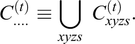$C_{x y z s}^{(t)}$ denote the value of C_xyzs after the tth case has been selected and let

C_{. . . .}^{(t)} \equiv ⋃_{x y z s} C_{x y z s}^{(t)} .

In the results that follow, we allow the probability that unit i is selected for analysis at time t $(S_{i}^{(t)} = 1)$ to depend on x_i , y_i , C ^(r), the researcher’s subjective beliefs about Z_i , and $s_{i}^{(r)}$ for r < t. We do not allow the selection probabilities to depend on the unknown value of z_i after the researcher has conditioned on the quantities in the previous sentence.

Our probability model for (X, Y, Z ) features two sets of parameters—θ and ψ. θ governs the multinomial distribution for (X, Y ) marginalized over Z, and ψ controls a series of binomial distributions for Z that are defined conditionally on X and Y. θ captures the descriptive association between X and Y, whereas ψ captures information that is purely causal (how the potential outcomes vary, given X and Y ). Table 3 provides details and interpretations of these parameters.

Table 3.

Interpretation of Parameters in the Model for (X, Y, Z ).

Parameter	Probability	Interpretation
θ _xy	$Pr (X_{i} = x, Y_{i} = y)$	Probability X_i is equal to x and Y_i is equal to y
ψ₀₀	$Pr (Z_{i} = 1 \| X_{i} = 0, Y_{i} = 0)$	Probability i would be helped by treatment, given i not treated and i failed
1 − ψ₀₀	$Pr (Z_{i} = 0 \| X_{i} = 0, Y_{i} = 0)$	Probability i would never succeed, given i not treated and i failed
ψ₀₁	$Pr (Z_{i} = 3 \| X_{i} = 0, Y_{i} = 1)$	Probability i would always succeed, given i not treated and i succeeded
1 − ψ₀₁	$Pr (Z_{i} = 2 \| X_{i} = 0, Y_{i} = 1)$	Probability i would be hurt by treatment, given i not treated and i succeeded
ψ₁₀	$Pr (Z_{i} = 2 \| X_{i} = 1, Y_{i} = 0)$	Probability i was hurt by treatment, given i treated and i failed
1 − ψ₁₀	$Pr (Z_{i} = 0 \| X_{i} = 1, Y_{i} = 0)$	Probability i would never succeed, given i treated and i failed
ψ₁₁	$Pr (Z_{i} = 3 \| X_{i} = 1, Y_{i} = 1)$	Probability i would always succeed, given i treated and i succeeded
1 − ψ₁₁	$Pr (Z_{i} = 1 \| X_{i} = 1, Y_{i} = 1)$	Probability i was helped by treatment, given i treated and i succeeded

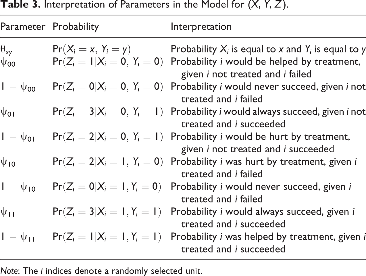
Note: The i indices denote a randomly selected unit.

Before writing out the posterior distribution for our parameters of interest, it is useful to introduce the notation 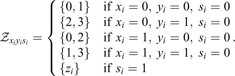$Z_{x_{i} y_{i} s_{i}}$ to represent a researcher’s knowledge of z_i , given realized values x_i , y_i , and s_i . Formally,

Z_{x_{i} y_{i} s_{i}} = \{\begin{matrix} \{0, 1\} & i f x_{i} = 0, y_{i} = 0, s_{i} = 0 \\ \{2, 3\} & i f x_{i} = 0, y_{i} = 1, s_{i} = 0 \\ \{0, 2\} & i f x_{i} = 1, y_{i} = 0, s_{i} = 0 \\ \{1, 3\} & i f x_{i} = 1, y_{i} = 1, s_{i} = 0 \\ \{z_{i}\} & i f s_{i} = 1 \end{matrix} .

Now we can write the posterior distribution of θ and ψ as: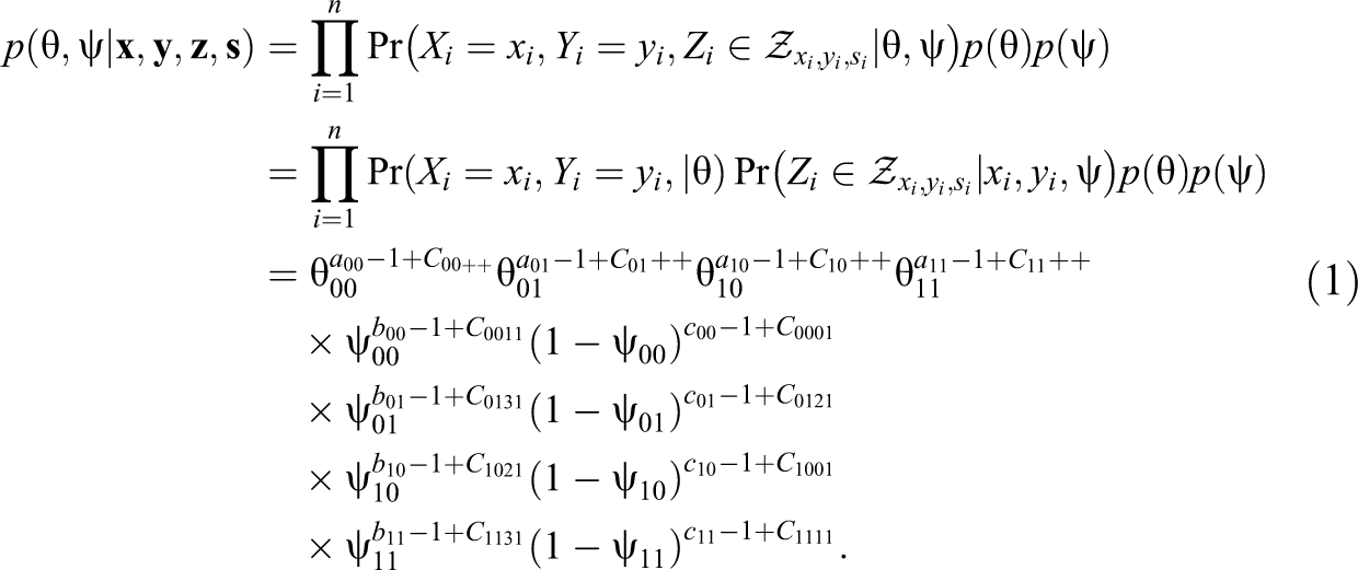

\begin{matrix} p (θ, ψ | x, y, z, s) = \prod_{i = 1}^{n} \Pr (X_{i} = x_{i}, Y_{i} = y_{i}, Z_{i} \in Z_{x_{i}, y_{i}, s_{i}} | θ, ψ) p (θ) p (ψ) \\ = \prod_{i = 1}^{n} \Pr (X_{i} = x_{i}, Y_{i} = y_{i}, | θ) \Pr (Z_{i} \in Z_{x_{i}, y_{i}, s_{i}} | x_{i}, y_{i}, ψ) p (θ) p (ψ) \\ = θ_{00}^{a_{00} - 1 + C_{00 + +}} θ_{01}^{a_{01} - 1 + C_{01} + +} θ_{10}^{a_{10} - 1 + C_{10} + +} θ_{11}^{a_{11} - 1 + C_{11} + +} \times \\ ψ_{00}^{b_{00} - 1 + C_{0011}} {(1 - ψ_{00})}^{c_{00} - 1 + C_{0001}} \times \\ ψ_{01}^{b_{01} - 1 + C_{0131}} {(1 - ψ_{01})}^{c_{01} - 1 + C_{0121}} \times \\ ψ_{10}^{b_{10} - 1 + C_{1021}} {(1 - ψ_{10})}^{c_{10} - 1 + C_{1001}} \times \\ ψ_{11}^{b_{11} - 1 + C_{1131}} {(1 - ψ_{11})}^{c_{11} - 1 + C_{1111}} . \end{matrix}

Note we assume that, a priori, $θ ~ D i r i c h l e t (a_{00}, a_{01}, a_{10}, a_{11})$ , $ψ_{x y} ~ b e t a (b_{x y}, c_{x y})$ with θ, ψ₀₀, ψ₀₁, ψ₁₀, ψ₁₁ are all mutually independent.

If ψ is known, we can write the average treatment effect as:

\begin{aligned} A T E = Pr (Y (X = 1) = 1) - Pr (Y (X = 0) = 1) \\ = (θ_{00} ψ_{00} + θ_{01} ψ_{01} + θ_{11}) - (θ_{10} ψ_{10} + θ_{11} ψ_{11} + θ_{01}) . \end{aligned}

This will be valid regardless of the pattern of confounding, but it does require knowledge of ψ (and SUTVA). In what follows, we choose to look at case selection as a way to learn about the conditional probability distribution of Z, given X and Y (i.e., ψ) and hence infer ATE. Bayesian inference for θ, ψ, and causal quantities such as ATE is straightforward but somewhat tedious. For details, see Quinn (2008).

Case Selection Methods

The analysis in Case Selection for Causal Effect Estimation subsection is predicated on knowing the realized values of Z_i for some (small) subset of units. Having noted this, we now attempt to operationalize a number of methods of case selection that have appeared in the qualitative methodology literature. The methods of case selection that we consider here are largely derived from the methods discussed in Gerring (2006) and Seawright and Gerring (2008). While it is not always unambiguously clear how, within the analytical framework of this article, to operationalize a particular case selection technique, we have tried to remain as faithful as possible to the spirit of Gerring’s suggestions. Nonetheless, it is important to be clear up front that our results and conclusions deal only with our very specific implementations of various case selection mechanisms. Thus, our conclusions about, say, influential case selection only apply to our specific implementation of this method and not to other case selection methods that might be referred to as influential case selection methods. We also emphasize that we evaluate these case selection methods in reference to their performance as part of a research strategy designed to infer effects of causes.

Although not necessarily advocated by Gerring, we include simple random sampling as a case selection technique. This is primarily for purposes of comparison. Random sampling provides a natural set of benchmarks for other case selection techniques, and in the remainder of this section, we discuss our implementation of the latter.

Typical Case Selection

Gerring (2006) writes:

In order for a focused case study to provide insight into a broader phenomenon, it must be representative of a broader set of cases. It is in this context that one may speak of a typical-case approach to case selection. The typical case exemplifies what is considered to be a typical set of values, given some general understanding of the phenomenon (p. 91).

And he goes on to state:

When a case falls close to the regression line, its typicality will be just below zero. When a case falls far from the regression line, its typicality will be far below zero. Typical cases have small residuals. (p. 94)

We operationalize Gerring’s typical case method of case selection in two ways. The first way, which we refer to as typical case selection, works as follows.

Note that the log odds ratio

ω = log (C_{00 + +}) + log (C_{11 + +}) - log (C_{01 + +}) - log (C_{10 + +}),

for a given (X, Y ) table contains information about the association between X and Y. In particular, if ω > 0, then there is a positive association between X and Y, if ω < 0, there is a negative association. If there is a positive association, that is, ω > 0, then we randomly sample cases for additional analysis from the main diagonal cells (X = 0, Y = 0) and (X = 1, Y = 1) with selection probabilities proportional to C ₀₀₊₊ and C ₁₁₊₊, respectively. If the association in the table is negative, we sample from the (X = 0, Y = 1) and (X = 1, Y = 0) cells with selection probabilities proportional to C ₀₁₊₊ and C ₁₀₊₊, respectively. This sampling protocol captures the essence of Gerring’s description of typical cases as lying close to the regression line.

A second way to define a typical case is to posit that such a case falls within the largest cell of an (X, Y ) table. For instance, if C ₀₀₊₊ > C ₁₀₊₊ > C ₀₁₊₊ > C ₁₁₊₊, then we would take a random sample of observations from the (X = 0, Y = 0) cell of the table for analysis. We refer to this method as largest cell selection.

Diverse Case Selection

Gerring (2006) writes:

A second case-selection strategy has as its primary objective the achievement of maximum variance along relevant dimensions. I refer to this as a diverse case method. For obvious reasons, this method requires the selection of a set of cases—at minimum, two—that are intended to represent the full range of values characterizing X ₁, Y, or some X ₁/Y relationship.

In the present context, we take this to mean that cases should be selected for analysis in such a way that keeps the total number of cases selected from each of the four cells of the (X, Y ) table as close to equal as possible. In our notation, this means that cases must be selected, so that C ₀₀₊₁ ≈ C ₀₁₊₁ ≈ C ₁₀₊₁ ≈ C ₁₁₊₁ with as many as possible of the equalities holding exactly.

We use the following sequential sampling method to achieve this goal. As stated previously, let Q denote the total number of cases to be selected for analysis, and let t = 1,…Q index the sequence of selections. When t = 1, 5, 9, …, pick one of the four cells of the (X, Y ) table with equal probability and randomly sample an observation from that cell. When t = 2, 6, 10, …, pick one of the three cells that was not sampled from iteration t − 1 with equal probability and randomly sample an observation from that cell. When t = 3, 7, 11, …, randomly pick one of the two cells that was not sampled from iteration t − 1or t − 2 with equal probability and sample an observation from that cell. When t = 4, 8, 12, …, randomly sample an observation from the cell that was not sampled from iteration t − 1, t − 2, or t − 3.

We call the method described previously as diverse case selection. Note that this way of operationalizing diverse case selection remains well defined for values of Q that are not evenly divisible by 4—including Q = 1. This is useful when we move on to a comparison of various case selection methods later in the article.

Extreme Case Selection

Gerring (2006) writes:

The extreme-case method selects a case because of its extreme value on an independent or dependent variable of interest…An extreme value is an observation that lies far away from the mean of a given distribution…For a dichotomous variable (present/absent), I understand extreme to mean unusual. If most cases are positive along a given dimension, then a negative case constitutes and extreme case. If most cases are negative, then a positive case constitutes an extreme case…It is the rareness of the value that makes a case valuable, in this context, not its positive or negative value (pp. 101-2).

We chose to operationalize this case selection method by randomly sampling observations from the smallest cell of the (X, Y ) table. Thus, if C ₁₀₊₊ < C ₁₁₊₊ < C ₀₁₊₊ < C ₀₀₊₊, we would randomly sample observations that have X = 1 and Y = 0. We refer to this selection method as extreme case selection.

Deviant Case Selection

Gerring (2006) writes:

The deviant-case method selects the case(s) that, by reference to some general understanding of a topic (either a specific theory or common sense), demonstrates a surprising value…The important point is that deviantness can only be assessed relative to the general (quantitative or qualitative) model employed…In statistical terms, deviant-case selection is the opposite of typical-case selection. Where a typical case lies as close as possible to the prediction of a formal, mathematical representation of the hypothesis at hand, a deviant case lies as far as possible from that prediction…Deviance ranges from 0, for cases exactly on the regression line, to a theoretical limit of infinity. Researchers will usually be interested in selecting from the cases with the highest overall estimated deviance (pp. 105-7).

Since Gerring views deviant case selection as the opposite of typical case selection, we operationalize our version of deviant case selection accordingly. As stated previously, the log odds ratio

ω = log (C_{00 + +}) + log (C_{11 + +}) - log (C_{01 + +}) - log (C_{10 + +})

is calculated for a given (X, Y ) table. As we discussed earlier, ω > 0 implies a positive association between X and Y, and ω < 0 implies a negative association. If there is a positive association, deviant case selection would have us randomly sample cases for additional analysis from the off diagonal cells (X = 0, Y = 1) and (X = 1, Y = 0) with selection probabilities proportional to C ₀₁₊₊ and C ₁₀₊₊, respectively. On the other hand, if the association in the table is negative, we sample from the (X = 0, Y = 0) and (X = 1, Y = 1) cells with selection probabilities proportional to C ₀₀₊₊ and C ₁₁₊₊, respectively.

Influential Case Selection

Gerring’s discussion of what he terms influential case selection is cast largely in terms of analogies to linear regression. While such ideas do not translate cleanly to the present context, we interpret Gerring’s discussion of this case selection method to be primarily concerned with selecting cases that minimize the sampling variability of one’s estimator—much as one would do under optimal model-based sampling designs; for example, see Glynn et al. (2008). Accordingly, we chose to define influential case selection as a case selection procedure that is part of a Bayesian decision problem whose goal is to minimize the posterior variance of the quantity of interest, here ATE.

Within the framework of this article, we operationalize influential case selection with the following adaptive sampling procedure. Once again, let t = 1,…Q index the sequence of case selection decisions. Let $C_{x y z s}^{(t)}$ denote the value of C_xyzs after the tth case has been selected. Sums over C_xyzs are similarly defined. Let

C_{. . . .}^{(t)} \equiv ⋃_{x y z s} C_{x y z s}^{(t)} .

Define:

η_{x y}^{(t)} \equiv E [V [A T E | C_{. . . .}^{(t)}] | C_{. . . .}^{(t - 1)}, C_{x y + 1}^{(t)} = C_{x y + 1}^{(t - 1)} + 1] .

In words, $η_{x y}^{(t)}$ is the expected posterior variance of the ATE, given the case selection that has occurred up to and including iteration t − 1 and the decision to take the tth sample from the (X = x, Y = y) cell of the table. Influential case selection is, for each t = 1, …, Q, choosing to randomly sample from the $(X = \tilde{x}, Y = \tilde{y})$ cell of the table, where $(\tilde{x}, \tilde{y}) = arg {min}_{x, y} η_{x y}^{(t)}$ . Note that the choice of which cell of the (X, Y ) table to select a case from at iteration t depends on what has been learned from case analysis at all previous iterations. Influential case selection is thus an adaptive sampling scheme.

Crucial (Most) Case Selection

Close reading of Gerring (2006) suggests that his crucial (most) case selection method depends on strong prior knowledge of the counterfactual outcomes of units. In our opinion, case selection methods that require accurate prior knowledge of the potential outcomes of units in order to work well are hard to rationalize—if one knows the potential outcomes of units, then one does not need to do any case selection to infer average causal effects.

Nonetheless, we have attempted to operationalize a case selection method that corresponds with a simple understanding of Gerring’s crucial case selection method, specifically what is written in table 5.1 of his book. Suppose $\tilde{y}$ and $y Ã µ$ are chosen, so that $C_{+ \tilde{y} + +} > C_{+ y Ã µ + +}$ . We define crucial (most) case selection as sampling cases from the $(X = 0, Y = \tilde{y})$ and $(X = 1, Y = \tilde{y})$ cells with probabilities proportional to $C_{0 \tilde{y} + +}$ and $C_{1 \tilde{y} + +}$ , respectively.

To be clear, we do not think that this case selection technique is what Gerring is discussing in the text of his 2006 book. Nonetheless, this does seem to loosely correspond to what is printed in table 5.1, and it is conceivable that some researchers would pursue similar case selection strategies in actual research situations. For instance, principle 1 of Goertz (2008) would have one look solely among the cases with Y = 1. While Goertz explicitly argues against random selection, his focus on examining cases with only a single Y-value is similar in spirit to our crucial (most) method (and the crucial (least) method discussed immediately below).

Crucial (Least) Case Selection

The same caveat that applies to our crucial (most) case selection method applies to what Gerring refers to as crucial (least) case selection. We operationalize crucial (least) case selection as follows. Suppose $\tilde{y}$ and $y Ã µ$ are chosen, so that $C_{+ \tilde{y} + +} > C_{+ y Ã µ + +}$ . Based on this, sample cases from the $(X = 0, Y = y Ã µ)$ and $(X = 1, Y = y Ã µ)$ cells with probabilities proportional to $C_{0 y Ã µ + +}$ and $C_{1 y Ã µ + +}$ , respectively. This selection method could be seen as another way to implement the extreme case selection method.

Case Selection via Simple Random Sampling

We also look at the properties of simple random sampling when applied to the problem at hand. This selection method can be conducted in the following way. First, randomly choose cell (X = x, Y = y) of the 2 × 2 table with probability proportional to C_xy ₊₊ for x = 0, 1 and y = 0, 1. Then randomly select a unit from this cell (with equal probability).

General Comments

All the case selection methods discussed previously are forms of (possibly stratified and possibly adaptive) random sampling. The only way that nonrandom sampling methods will perform well is if a researcher has a great deal of background knowledge about the distribution of potential outcomes of interest (the ψ parameter). However, methods that require accurate prior knowledge about potential outcomes to perform well do not require any case selection to be done at all since accurate knowledge of ψ and θ is sufficient to accurately infer ATE.

Monte Carlo Experiments

To evaluate the nine methods of case selection discussed previously across a variety of plausible scenarios, we conduct 12 Monte Carlo experiments. These 12 experiments vary the degree to which the elements of θ are of similar size, the degree of confounding (if any), and the direction of any confounding bias that does exist; and, for the cases where there is no confounding bias, the distribution of the potential outcomes that results in mean ignorability. Although the size of the elements of θ changes across experiments, we maintain $θ_{01} / (θ_{00} + θ_{01}) = 0.4$ and $θ_{11} / (θ_{10} + θ_{11}) = 0.6$ . This keeps the prima facie ATE, defined as $A T E_{p f} \equiv Pr (Y = 1 | X = 1) - Pr (Y = 1 | X = 0)$ , constant at 0.2 across Monte Carlo experiments. It is also the case that the large-sample, nonparametric bounds on ATE remain constant at [−0.4, 0.6] across experiments.

Each of the 12 Monte Carlo experiments was conducted in the following fashion.

1. Set θ₀₀, θ₀₁, θ₁₀, θ₁₁, ψ₀₀, ψ₀₁, ψ₁₀, ψ₁₁, first-stage sample size N, and second-stage sample size Q. Also, choose a case selection method.

2. For m = 1,…, M

Randomly generate C_xyz ₊ from the appropriate distribution, given the fixed values of θ and ψ from step 1 above. Do this for all x, y, and z.

Sample Q cases for analysis using the case selection method chosen in step 1. The z values for these units become observed.

Using the data generated in steps 2(a) and 2(b), calculate the posterior distribution of (θ, ψ) and then use this information to calculate and summarize the implied posterior distribution for ATE. Save the ATE posterior summaries.

3. Summarize the performance of the case selection method under study over the M data sets to which it was applied.

Our results are based on N = 10,000, M = 1,000, and $Q \in \{1, 3, 5, 7, 10, 15, 20\}$ . The values of θ and ψ used in the 12 experiments, along with the implied true value of ATE, the prima facie ATE, and the associated degree of confounding bias are all presented in Table 4. In all experiments, we assume the following priors: $θ ~ D i r i c h l e t (0.25, 0.25, 0.25, 0.25)$ and $ψ_{x y} ~ b e t a (0.5, 0.5)$ for x = 0, 1 and y = 0,1.

Table 4.

Summary of Monte Carlo Experiments.

											Confounding
Experiment #	θ₀₀	θ₀₁	θ₁₀	θ₁₁	ψ₀₀	ψ₀₁	ψ₁₀	ψ₁₁	ATE _true	ATE _pf	Bias
1	0.3	0.2	0.2	0.3	0.6	0.6	0.6	0.267	0.2	0.2	0.00
2	0.3	0.2	0.2	0.3	0.9	0.15	0.1	0.6	0.2	0.2	0.00
3	0.3	0.2	0.2	0.3	0.7	0.7	0.3	0.3	0.3	0.2	–0.10
4	0.3	0.2	0.2	0.3	0.5	0.5	0.5	0.5	0.1	0.2	+0.10
5	0.3	0.2	0.2	0.3	0.99	0.99	0.01	0.01	0.59	0.2	–0.39
6	0.3	0.2	0.2	0.3	0.01	0.01	0.99	0.99	−0.39	0.2	+0.59
7	0.546	0.364	0.036	0.054	0.6	0.6	0.6	0.267	0.2	0.2	0.0
8	0.546	0.364	0.036	0.054	0.9	0.15	0.1	0.6	0.2	0.2	0.0
9	0.546	0.364	0.036	0.054	0.7	0.7	0.3	0.3	0.3	0.2	–0.10
10	0.546	0.364	0.036	0.054	0.5	0.5	0.5	0.5	0.1	0.2	+0.10
11	0.546	0.364	0.036	0.054	0.99	0.99	0.01	0.01	0.59	0.2	–0.39
12	0.546	0.364	0.036	0.054	0.01	0.01	0.99	0.99	−0.39	0.2	+0.59

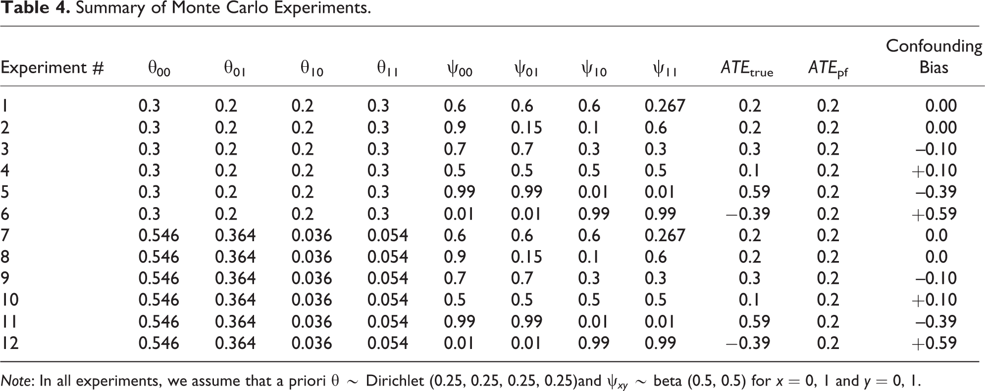
Note: In all experiments, we assume that a priori θ ∼ Dirichlet (0.25, 0.25, 0.25, 0.25)and ψ _xy ∼ beta (0.5, 0.5) for x = 0, 1 and y = 0, 1.

We look at four quantities to gauge the performance of the case selection schemes under study: bias, frequentist RMSE, posterior variance, and posterior RMSE. Let D_m denote all of the prior parameters and observed data from Monte Carlo replication m and 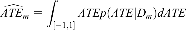$p (A T E | D_{m})$ denote the posterior distribution of ATE, given the observed data from Monte Carlo replication m and let

{\hat{A T E}}_{m} \equiv \int_{[- 1, 1]} A T E p (A T E | D_{m}) d A T E

denote the posterior mean of ATE in the mth Monte Carlo replication under a particular case selection scheme.

Traditional frequentist criteria of bias and RMSE are defined as: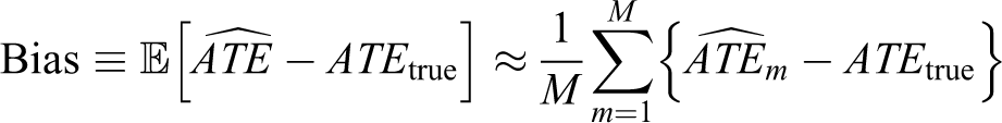

B i a s \equiv E [\hat{A T E} - A T E_{t r u e}] \approx \frac{1}{M} \sum_{m = 1}^{M} \{{\hat{A T E}}_{m} - A T E_{t r u e}\}

and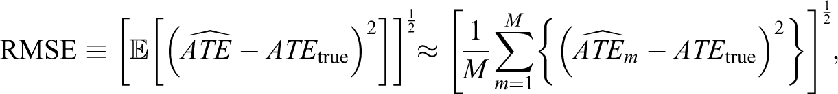

R M S E \equiv {[E [{(\hat{A T E} - A T E_{t r u e})}^{2}]]}^{\frac{1}{2}} \approx {[\frac{1}{M} \sum_{m = 1}^{M} \{{({\hat{A T E}}_{m} - A T E_{t r u e})}^{2}\}]}^{\frac{1}{2}},

where the last terms give the Monte Carlo estimates of these quantities. Criteria with more of a Bayesian flavor include the posterior variance of ATE:

{P o s t e r i o r V a r i a n c e}_{m} \equiv \int_{[- 1, 1]} {(A T E - {\hat{A T E}}_{m})}^{2} p (A T E | D_{m}) d A T E

and the posterior RMSE: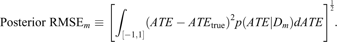

P o s t e r i o r {R M S E}_{m} \equiv {[\int_{[- 1, 1]} {(A T E - A T E_{t r u e})}^{2} p (A T E | D_{m}) d A T E]}^{\frac{1}{2}} .

Note that these quantities are defined for an individual Monte Carlo replication m. In what follows, we will look at the distribution of these quantities over all M Monte Carlo replications

In a perfect world, a case selection technique will have bias close to 0 and low RMSE, posterior variance, and posterior RMSE. This statement provides absolute standards for a case selection method. Selection methods can also be compared to each other, as we show subsequently.

Bias

Figures 1 and 2 display the biases of the various case selection methods across the different data-generating processes and sample sizes. When confounding is absent and the (X, Y ) cells are of similar size (experiments 1 and 2), then all methods perform similarly with a slight edge going to typical case selection, diverse case selection, influential case selection, and simple random sampling. However, when the (X, Y ) cells are not of similar size and the prior for ψ is not close to the true value of ψ (experiment 8), then methods other than typical case selection, influential case selection, or simple random sampling do poorly—in some cases increasingly poorly as the sample size gets large. With moderate or severe confounding, methods other than typical case selection, influential case selection, or simple random sampling also do poorly. Again the disparity in performance between these methods and the others grows as the sample size gets larger.

Figure 1.

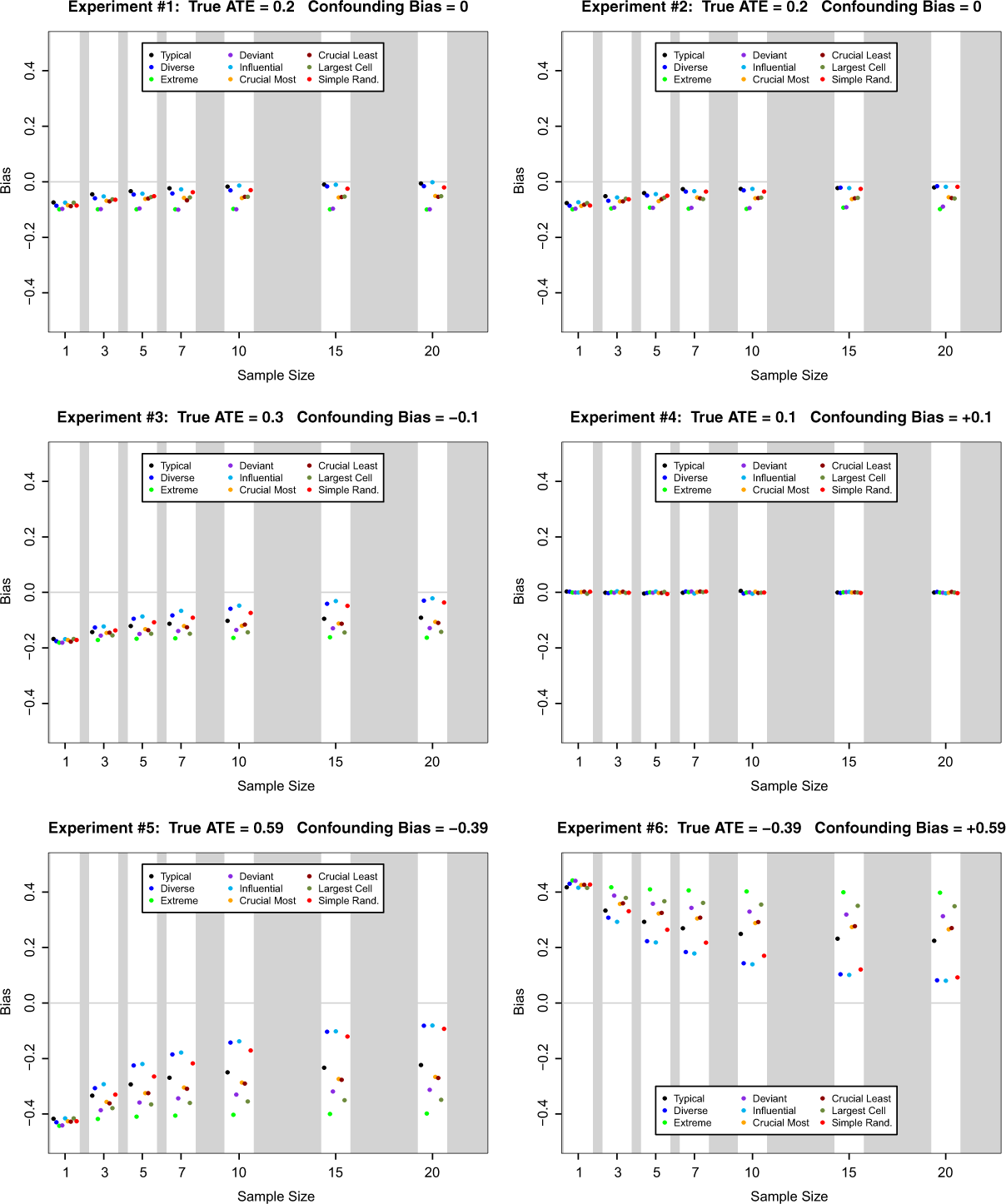
Bias of posterior mean estimator of ATE for nine case selection schemes and seven sample sizes in Monte Carlo experiments 1 through 6. Here the cells of the (X, Y ) table are relatively balanced with θ₀₀ = 0.3, θ₀₁ = 0.2, θ₁₀ = 0.2, and θ₁₁ = 0.3.

Figure 2.

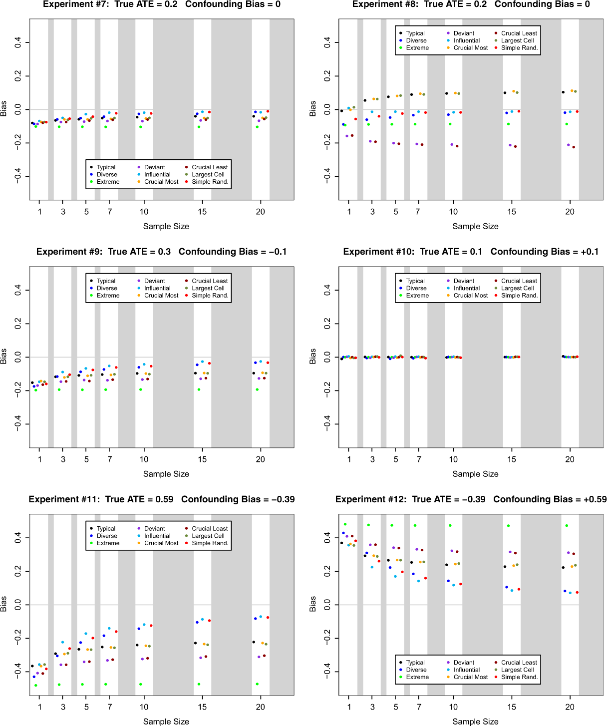
Bias of posterior mean estimator of ATE for nine case selection schemes and seven sample sizes in Monte Carlo experiments 7 through 12. Here the cells of the (X, Y ) table are relatively unbalanced with θ₀₀ = 0.546, θ₀₁ = 0.364, θ₁₀ = 0.036, and θ₁₁ = 0.054.

It is worth noting that for relatively small sample sizes of 3 and 5, influential case selection exhibits noticeably less bias than other methods. However, it is also worth noting that simple random sampling—often maligned as inappropriate for small-Q (qualitative) case study research—has lower bias than most other case selection methods. Of course, many would argue that this is not surprising and that the real reason for not using simple random sampling is its relatively high variance and high RMSE. We examine the accuracy of this belief subsequently. Finally, we note that bias is low for all case selection methods in experiments 4 and 10 because the prior distribution used in the experiments is (coincidentally) centered on the true value of ATE.

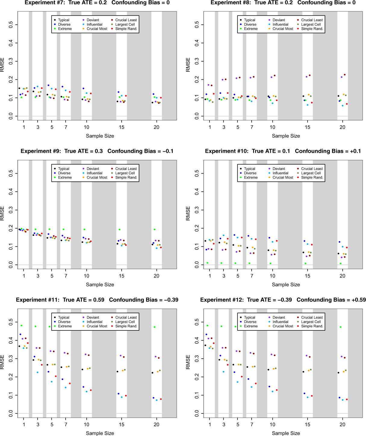
RMSE

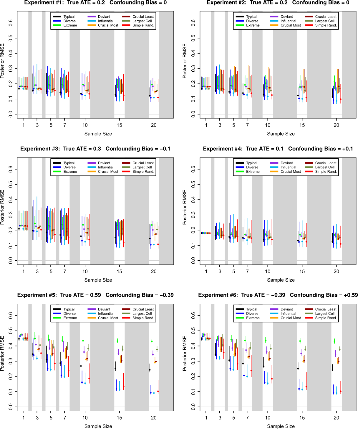
Figures 3 and 4 display the RMSE of the various case selection methods across the various Monte Carlo experiments. For the experiments in which confounding is either moderate or absent, no sampling scheme dominates in terms of RMSE. Our hypothesis for why this is the case is that frequentist RMSE looks only at the sampling distribution of our point estimator (here the posterior mean) and this will depend heavily on the prior. For instance, RMSE is low for case selection methods that select cases from small (X, Y ) cells in experiments 4 and 10 because the prior distribution used in the experiments is (coincidentally) centered on the true value of ATE. Sampling in a way that does little to change the posterior from the prior will only have good properties when, as is the case in these experiments, the prior is centered on the truth.

Figure 3.

Root mean square error (RMSE) of posterior mean estimator of ATE for nine case selection schemes and seven sample sizes in Monte Carlo experiments 1 through 6. Here the cells of the (X, Y ) table are relatively balanced with θ₀₀ = 0.3, θ₀₁ = 0.2, θ₁₀ = 0.2, and θ₁₁ = 0.3.

Figure 4.

Root mean square error (RMSE) of posterior mean estimator of ATE for nine case selection schemes and seven sample sizes in Monte Carlo experiments 7 through 12. Here the cells of the (X, Y ) table are relatively unbalanced with θ₀₀ = 0.546, θ₀₁ = 0.364, θ₁₀ = 0.036, and θ₁₁ = 0.054.

When the degree of confounding becomes severe (experiments 5, 6, 11, and 12) a clearer picture emerges. With similarly sized (X, Y ) cells (experiments 5 and 6) and moderate sample sizes (Q = 3, 5, 7), both diverse and influential case selection perform much better than the alternatives. In these situations, simple random sampling becomes increasingly attractive as Q gets larger. With very different (X, Y ) cell sizes, (experiments 11 and 12), and moderate sample sizes (Q = 3, 5, 7), influential case selection performs better than the alternatives, with simple random sampling coming in second. Diverse case selection closes the gap as Q gets larger. In situations with severe confounding, the case selection methods that focus on relatively unpopulated (X, Y ) cells do extremely poorly in terms of RMSE.

Posterior Variance

Figures 5 and 6 summarize the distribution of the posterior variance of ATE for the various sampling schemes, sample sizes, and data-generating processes. While the posterior variance is of limited interest in its own right (a certain case selection method might often produce low posterior variance but be very far from the truth), it does allow us to see which case selection methods produce the largest changes from prior to posterior. In some sense, this is a measure of how much learning has occurred under a particular case selection scheme.

Figure 5.

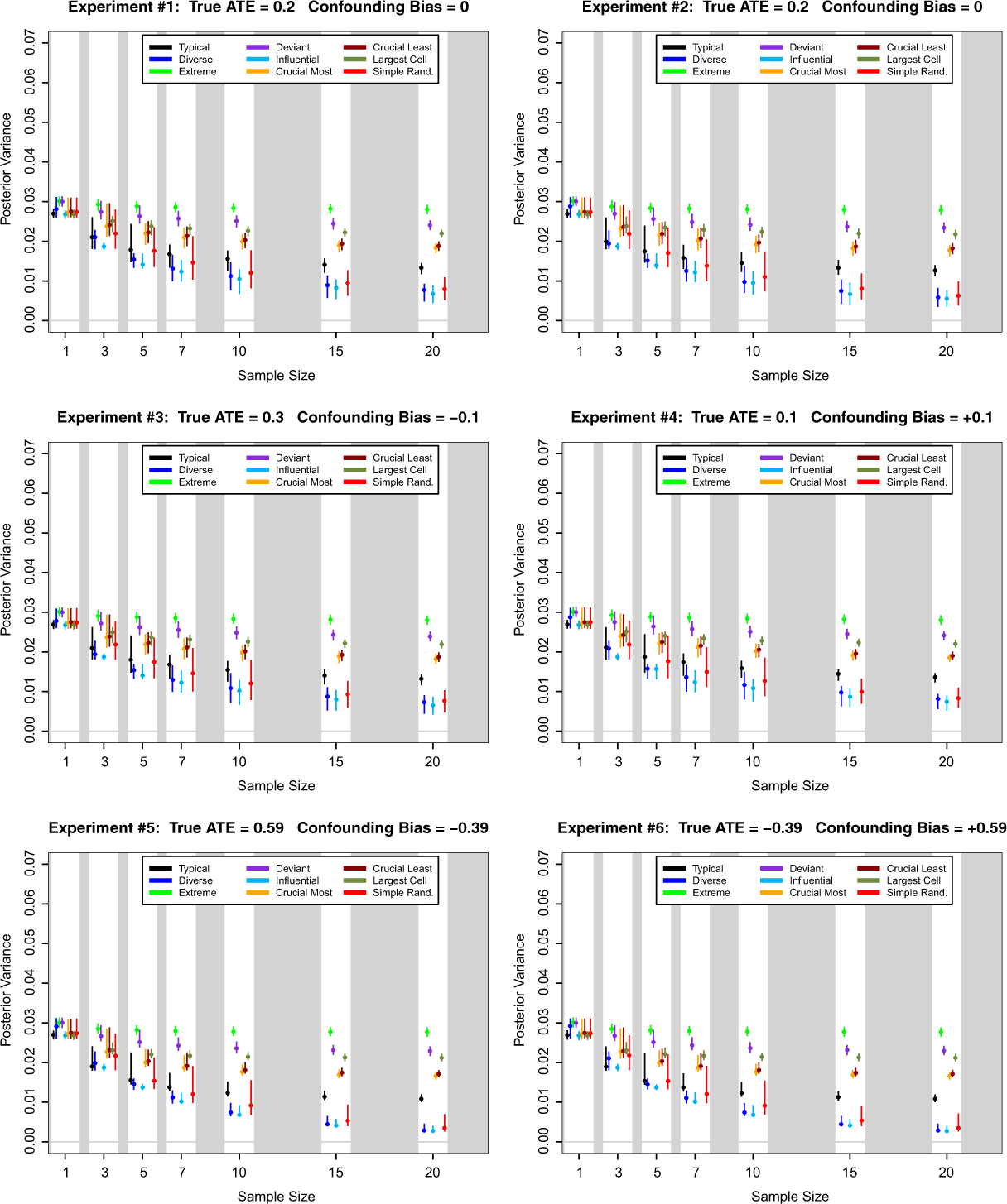
Posterior variance of ATE for nine case selection schemes and seven sample sizes in Monte Carlo experiments 1 through 6. Here the cells of the (X, Y ) table are relatively balanced with θ₀₀ = 0.3, θ₀₁ = 0.2, θ₁₀ = 0.2, and θ₁₁ = 0.3. Dots are median values over 1,000 simulations and line segments are central 95 percent regions.

Figure 6.

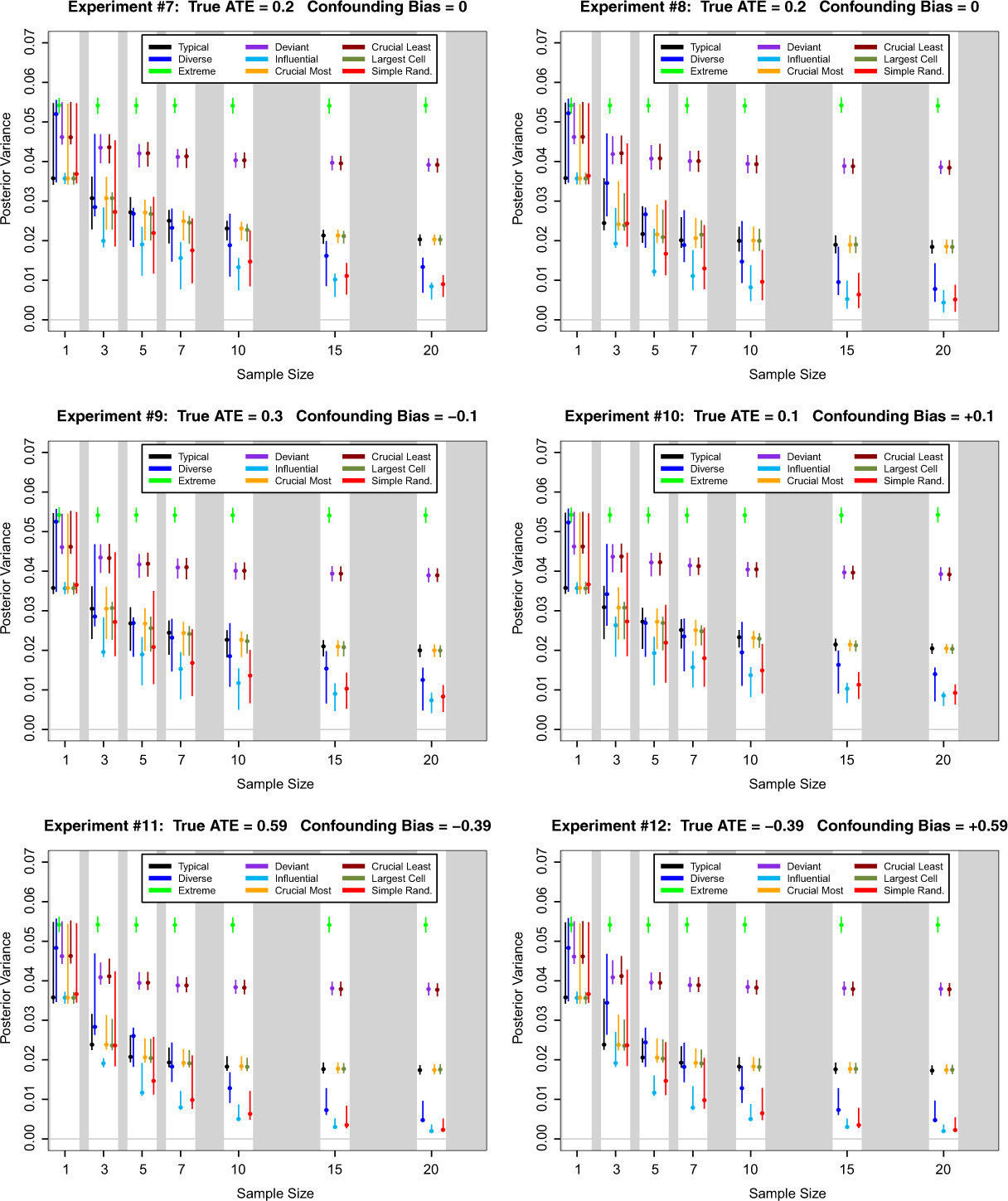
Posterior variance of ATE for nine case selection schemes and seven sample sizes in Monte Carlo experiments 7 through 12. Here the cells of the (X, Y ) table are relatively unbalanced with θ₀₀ = 0.546, θ₀₁ = 0.364, θ₁₀ = 0.036, and θ₁₁ = 0.054. Dots are median values over 1,000 simulations and line segments are central 95 percent regions.

The results here are quite unambiguous—influential case selection does the most to shrink the posterior variance of ATE. This is true across all values of Q in all the Monte Carlo experiments. This should not be too surprising since our operationalization of influential case selection was designed to minimize posterior variance of ATE. Nevertheless, it is instructive to see how much better influential case selection is in this regard than other case selection methods. It is also very interesting to note that simple random sampling also fares quite well in terms of posterior variance. This is the case even with fairly moderate sample sizes (Q = 5, 7). It thus seems that some of the concerns regarding the assumed high variance of simple random sampling with moderate sample sizes are misplaced.

Posterior RMSE

Figures 7 and 8 summarize across Monte Carlo experiments the distribution of the posterior RMSE for the nine sampling schemes under study. In many ways, low posterior RMSE is of most relevance to applied researchers, as it measures how close the entire posterior distribution is to the truth rather than just the proximity of a point estimator to the truth.

Figure 7.

Posterior root mean square error (RMSE) of ATE for nine case selection schemes and seven sample sizes in Monte Carlo experiments 1 through 6. Here the cells of the (X, Y ) table are relatively balanced with θ₀₀ = 0.3, θ₀₁ = 0.2, θ₁₀ = 0.2, and θ₁₁ = 0.3. Dots are median values over 1,000 simulations and line segments are central 95 percent regions.

Figure 8.

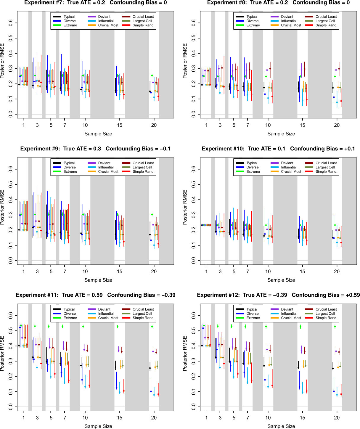
Posterior root mean square error (RMSE) of ATE for nine case selection schemes and seven sample sizes in Monte Carlo experiments 7 through 12. Here the cells of the (X, Y ) table are relatively unbalanced with θ₀₀ = 0.546, θ₀₁ = 0.364, θ₁₀ = 0.036, and θ₁₁ = 0.054. Dots are median values over 1,000 simulations and line segments are central 95 percent regions.

Once again, influential case selection emerges as the dominant case selection method. This is true across sample sizes and Monte Carlo experiments. The gains to using influential case selection are greatest when there is severe confounding and moderate to small sample sizes. When the (X, Y ) cells are of roughly equal size, diverse case selection does nearly as well as influential case selection. When the (X, Y ) cells are of very different sizes, then simple random sampling is second best. However, the largest posterior RMSE that one might see under simple random sampling can be noticeably higher than the largest posterior RMSE under influential case selection. Finally, it is worth noting that extreme case selection always does quite poorly when judged in terms of posterior RMSE. Based on these simulation results, it seems prudent to recommend that extreme case selection should not be used if the goal is to infer population-level average causal effects.

Summary of Monte Carlo Results

The message that applied researchers should take from our simulations is that our implementation of influential case selection is stronger on more criteria across more types of data-generating processes than other case selection methods. Influential case selection appears to be the best way to select cases if the goal of such case selection is to infer population-level average causal effects. Our implementation of diverse case selection and simple random sampling also fare quite well. Given that these latter methods are easier to implement that influential case selection, there is some argument for preferring these methods in certain situations. The fact that simple random sampling outperforms most methods of case selection—even when sample size is as small as 5 or 7—should be news to many (qualitative) researchers who assert that simple random sampling should only be used with relatively large, say Q > 20, sample sizes. Finally, if one can only choose a very small number of cases, say fewer than three, for case analysis, then the very simple method of randomly choosing cases from the largest cell of the 2 × 2 (X, Y ) table (largest cell case selection) is extremely competitive with other, more complicated, cases selection strategies.

The simulation results also set forth some clear messages about which case selection methods should always be avoided. Our implementation of extreme case selection always does extremely poorly unless one is lucky enough to know the answer (and encode this in one’s prior distribution) before the analysis begins. Similarly, deviant case selection and crucial (least) case selection generally fare quite poorly. The commonality shared by all three of these case selection methods is a focus on sparsely populated cells in the 2 × 2 (X, Y ) table. From a purely statistical sampling perspective, focusing attention on cases that are not representative of the population as a whole will usually lead to a huge waste of resources. While such cases may be useful for exploratory analysis and/or theory construction, the amount of information they can provide about population-level average causal effects is, by definition, limited.

Conclusion

Case study methodology is widely used by empirical social scientists, especially by qualitative researchers in the subfields of political science known as comparative politics and international relations. The fundamental issue involved with this methodology is how one should choose cases for detailed analysis. While a great deal has been written about case selection, there is still widespread disagreement regarding which case selection technique is optimal and in what circumstances. We believe that part of the reason for this lack of agreement stems from the lack of a rigorous counterfactual causal framework for case study research, and with this dearth in mind, we have provided such a framework.

We have used our framework to evaluate a number of prominent case selection methods that have been discussed at length by Seawright and Gerring. Our results suggest that our implementation of influential case selection is generally to be preferred over the other case selection methods under study. We also find that deviant case selection works quite well and that, contrary to conventional wisdom, simple random sampling performs well relative to most other case selection methods as long as a moderate number (say five or more) of cases are to be selected for case study analysis. Our findings have clear implications for how applied researchers should select cases for analysis, and extending our analytical approach to additional case selection techniques will help shed light on the best techniques in a variety of research situations. That said, we again emphasize that our results only speak directly to our stated goal of inferring effects of causes.

Footnotes

Acknowledgment

We thank Oliver Bevan, Adam Glynn, and Gary King for helpful conversations and the National Science Foundation (grants BCS 05-27513 and SES 07-51834) for research support. The authors are listed in alphabetic order.

Declaration of Conflicting Interests

The author(s) declared no potential conflicts of interest with respect to the research, authorship, and/or publication of this article.

Funding

The author(s) disclosed receipt of the following financial support for the research, authorship, and/or publication of this article: Kevin Quinn. National Science Foundation (grants BCS 05-27513 and SES 07-51834).

Notes

References

Chickering

David Maxwell

Pearl

Judea

. 1997. “A Clinician's Tool for Analyzing Non-compliance.” Computing Science and Statistics 29:424–31.

Fearon

James

. 1991. “Counterfactuals and Hypothesis Testing in Political Science.” World Politics 43:474–84.

Ferguson

Niall

. 1999. Virtual History: Alternatives and Counterfactuals. New York: Basic Books.

Gerring

John

. 2004. “What Is a Case Study and What Is It Good for?” American Political Science Review 98:341–54.

Gerring

John

. 2006. Case Study Research: Principles and Practices. New York: Cambridge University Press.

Glynn

Adam N.

Quinn

Kevin M.

. 2011. “Why Process Matters for Causal Inference.” Political Analysis 19:273–86.

Glynn

Adam N.

Wakefield

Jon

Handcock

Mark S.

Richardson

Thomas S.

. 2008. “Alleviating Linear Ecological Bias and Optimal Design with Subsample Data.” Journal of the Royal Statistical Society, Series A 171:179–202.

Goertz

Gary

. 2008. “Choosing Cases for Case Studies: A Qualitative Logic.” Qualitative & Multi-Method Research 6:11–14.

Hawthorn

Geoffrey

. 1993. Plausible Worlds: Possibility and Understanding in History and the Social Sciences. New York: Cambridge University Press.

10.

Holland

Paul W.

1986. “Statistics and Causal Inference.” Journal of the American Statistical Association 81:945–60.

11.

Lebow

Richard Ned

. 2000. “Review: What’s So Different about a Counterfactual?” World Politics 52:550–85.

12.

Levy

Jack S.

2008. “Counterfactuals and Case Studies.” Pp. 627–44 in The Oxford Handbook of Political Methodology, edited by Box-Steffensmeier

Janet M.

Brady

Henry E.

Collier

David

. Oxford, UK: Oxford University Press.

13.

Licklider

Roy

. 1995. “The Consequences of Negotiated Settlements in Civil Wars, 1945-1993.” American Political Science Review 89:681–90.

14.

Neyman

Jerzy

Iwaszkiewicz

with K.

Kolodziejczyk

. 1935. “Statistical Problems in Agricultural Experimentation.” Supplement of Journal of the Royal Statistical Society 2:107–80.

15.

Pearl

Judea

. 1995. “Causal Diagrams for Empirical Research.” Biometrika 82:669–710.

16.

Pearl

Judea

. 2000. Causality: Models, Reasoning, and Inference. New York: Cambridge University Press.

17.

Quinn

Kevin M.

2008. “What Can Be Learned from a Simple Table? Bayesian Inference and Sensitivity Analysis for Causal Effects from 2 × 2 and 2 × 2 × K Tables in the Presence of Unmeasured Confounding.” Harvard University Working Paper, Harvard University, Cambridge, MA.

18.

Robins

James M.

1986. “A New Approach to Causal Inference in Mortality Studies with a Sustained Exposure Period-application to Control of the Healthy Worker Survivor Effect.” Mathematical Modeling 7:1393–512.

19.

Rubin

Donald B.

1974. “Estimating Causal Effects of Treatments in Randomized and Nonrandomized Studies.” Journal of Educational Psychology 66:688–701.

20.

Rubin

Donald B.

1978. “Bayesian Inference for Causal Effects: The Role of Randomization.” The Annals of Statistics 6:34–58.

21.

Seawright

Jason

Gerring

John

. 2008. “Case Selection Techniques in Case Study Research: A Menu of Qualitative and Quantitative Options.” Political Research Quarterly 61:294–308.

22.

Sekhon

Jasjeet S.

2004. “Quality Meets Quantity: Case Studies, Conditional Probability, and Counterfactuals.” Perspectives on Politics 2:281–93.