Phantom Effects in Multilevel Compositional Analysis

Abstract

This article combines statistical and applied research perspective showing problems that might arise when measurement error in multilevel compositional effects analysis is ignored. This article focuses on data where independent variables are constructed measures. Simulation studies are conducted evaluating methods that could overcome the measurement error problems. These methods are a multilevel regression model with reliability correction, a multilevel model with plausible values, and a multilevel latent regression model (doubly latent model). While the latter one performs best, all models have their advantages and disadvantages. Examples using data from the Trends in International Mathematics and Science Study are shown to present the behavior of the tested models in real-data situations and indicate the consequences of ignoring the problem of reliability.

Keywords

measurement error multilevel modeling simulation studies

Introduction

Compositional effects nowadays are in the spotlight of researchers from various fields of science. Sociologists and psychologists inquire how properties of the group affect individual decisions. Epidemiologists pursue health-determinant patterns. Economists try to find conditions that influence productivity and labor costs. Educational researchers seek compositional effects that moderate school achievements—like classroom or peer effects. All these questions are examined frequently in a multilevel modeling framework where individual outcomes are modeled by both individual- and group-level covariates where the latter are aggregations of individual covariates. In the very simple case, compositional analysis may be expressed formally by a two-level model (following Raudenbush and Bryk’s 2002 notation):

\begin{array}{l} I n d i v i d u a l l e v e l (1) : y_{i j} = β_{0 j} + β_{1 j} x_{i j} + r_{i j} \\ w h e r e : \\ G r o u p l e v e l (2) : β_{0 j} = γ_{00} + γ_{01} {\overset{ˉ}{x}}_{j} + u_{0 j} \\ β_{1 j} = γ_{10} \end{array}

Or in one equation:

y_{i j} = γ_{00} + γ_{10} x_{i j} + γ_{01} {\overset{ˉ}{x}}_{j} + u_{0 j} + r_{i j},

where y_ij is an outcome variable of individual i in group j; x_ij is an individual covariate;

{\overset{ˉ}{x}}_{j}

is a group-level covariate (aggregation of x_ij over group); r_ij and u_0j are residuals at level 2 and level 1, respectively (assumed to be independently distributed with zero mean and constant variance), and γ₀₀, γ₁₀, and γ₀₁ are fixed effects (intercept, individual effect, and compositional effect).

In equations (1) and (2), the parameter next to the individual-level variable (x_ij) is considered as an individual effect (γ₁₀), and the parameter next to the group-level covariate ( ${\overset{ˉ}{x}}_{j}$ ) is considered as a compositional effect (γ₀₁). For instance, a researcher may investigate the relationship between student performance and individual parental socioeconomic status together with average parental socioeconomic status in the classroom. The effect of parental socioeconomic status on student performance is called individual because it refers to individual attributes of the student (this student has a particular family background). The effect of average socioeconomic parental status on the student performance is called compositional because it refers to an attribute of the group that is made up of a composition of features belonging to individuals. Both effects have strong theoretical and commonsense justification and both are plausible to consider.

If all assumptions of multilevel models are met and variables are centered to the sample mean (as opposed to group mean centered), the multilevel model presented in equations (1) and (2) would produce unbiased parameters for both individual and compositional effects. The literature on multilevel modeling focuses mainly on assumptions of normality and linearity and attaches great importance to investigating whether residuals at each level are normally distributed, uncorrelated at each level and across levels, and equally distributed across x’s at each level and across levels (Maas and Hox 2004; Hox 2010:22-23; Raudenbush and Bryk 2002:35; Snijders and Bosker 1999:120-39). The assumptions—requiring no omitted variables (Kim and Frees 2006) and that variables are measured without error (Woodhouse et al. 1996)—often go unnoticed.

This article focuses on violation of the perfect reliability assumption (i.e., violation of the assumption that a variable is measured without a measurement error) and its impact on compositional effect estimation. To realize the problem of measurement error, one must recognize that in many cases, variables that researchers want to utilize are not directly observable. In such situations, proxy variables are used. Researchers want to analyze such things as weight, height, blood pressure, cognitive outcomes, personality traits, or income. But the variables are only representations of actual constructs; they are indicated by readings on scales, readings on sphygmomanometer, scores from cognitive tests or noncognitive questionnaires, or responses to a single question. It is well known that measuring instruments are not perfectly reliable. Test scores do not reflect abilities exactly, as scores depend on item selection for the test (quality and validity of items). Scores are discrete number of points, and ability is assumed to be continuous; moreover, the questions are correlated with ability in a diverse and limited range. Tests and questionnaires among many other things are affected by differences in students’ motivation and emotional state (Wolf, Smith, and Birnbaum 1995) and the health of respondents at the time of testing (Gronlund 1998). The particular mode of administration can also affect measurement (Bowling 2005). There are also other factors that might affect measurement, for instance: Recording income depends on how the question was interpreted by the respondent, how good his or her memory is, how willing he or she is to answer the question, and how efficient the interviewer is in writing down the answers of the respondent. In some cases, the measurement error might be very small and negligible as in weight and high measurement; in other situations, as in cognitive tests and psychological questionnaires, substantial measurement error is a rule rather than an exception. This fact is often forgotten while conducting statistical analysis. In some cases, as it will be shown later, ignoring measurement error brings about substantial biases in analysis and leads to false conclusions.

The problem of measurement error in one-level analysis was investigated early in statistics and econometric literature (Degracie and Fuller 1972; Fuller 1987; Madansky 1959; Maddala 1992; Shear and Zumbo 2013). In the case of multilevel models, the literature is much scarcer. There are articles that introduce the problem and propose some solutions (Longford 1993; Woodhouse et al. 1996; Yuan and Bentler 2004), but they are highly technical and do not show convincingly the practical consequences of violation of measurement error assumptions in a way that would be accessible to nontechnical audiences. They also lack extensive testing of proposed solutions, and are instead concerned with statistical details of estimation mechanisms, which are not implemented in widely available software. Very few articles present reasonable applicable and tested solutions (with some exceptions like the articles on contextual effects in the framework of structural equation models [SEMs] by Marsh and Hau 2003; Marsh et al. 2009).

In applied research literature, on the other hand, it was noted that measurement error in contextual analysis may produce fake compositional effects, so-called phantom effects (Harker and Tymms 2004; Thomas and Mortimore 1996; Tymms 1992:188, 190-91). Phantom effects are products of statistical methods not designed to deal with a situation involving data where measurement error is substantial. In applied research literature, authors show that a reckless approach to the assumptions of the statistical models might adversely affect conclusions. However, no systematic studies on this problem, with sufficient statistical explanation or satisfactory solution to cope with this problem, were provided. This article tries to bridge the gap between statistical theory and applied research by showing the problem and providing a set of practical solutions.

Many recent articles examining compositional effects ignore the problem of measurement error. Dedrick et al. (2009) analyzed the reporting of multilevel modeling applications of a sample of 99 articles from 13 peer-reviewed journals in education and the social sciences and showed that only 18 articles considered the potential impact of measurement error on the resulting models. It is not mentioned how many of them try to solve the problem.

Measurement Error and Intraclass Correlation (ICC)

The effect of measurement error on estimation of regression parameters might be easily shown in a simple one-level regression example with one explanatory variable:

y_{i} = β x_{i} + e_{i} .

Equation (3) expresses the relation between the dependent variable y_i, the independent observed variable x_i through a parameter β, and e_i stands for model error. For simplicity, we assume that both variables are continuous and standardized; therefore, there is no need to include a constant term in the regression. This model reflects an ideal situation where measurement error of x is absent. However, in most cases, variables are not observed directly— x_i comprises the true value $x_{i}^{'}$ and an error term m_i, while y_i comprises the true value $y_{i}^{'}$ and an error term n_i, so that equation (3) in order to reflect true relation between $y_{i}^{'}$ and $x_{i}^{'}$ might be rewritten as:

y_{i}^{'} + n_{i} = β (x_{i}^{'} + m_{i}) + e_{i} .

Under classical measurement error assumptions where:

\begin{array}{l} E (m_{i}) = 0; E (n_{i}) = 0; var (m_{i}) = σ_{m}^{2}; var (n_{i}) = σ_{n}^{2}; cov (x_{i}, y_{i}) = σ_{x y}; \\ cov (m_{i}, x_{i}) = cov (m_{i}, y_{i}) = cov (n_{i}, x_{i}) = cov (n_{i}, y_{i}) = cov (n_{i}, m_{i}) = 0. \end{array}

It can be easily shown that in ordinary least squares regression, the true relation between $x_{i}^{'}$ and $y_{i}^{'}$ will be underestimated because:

\hat{β} = σ_{x y} / σ_{x}^{2} = σ_{x y} / (σ_{x^{'}}^{2} + σ_{m}^{2}) < σ_{x y} / σ_{x^{'}}^{2} .

This underestimation is affected by measurement error in x_i but not in y_i (as errors do not affect covariance with classical measurement error assumptions). The bias in the parameter $\hat{β}$ might be easily corrected if the reliability (α) of the variable x_i is known: $β = \hat{β} / α$ , where reliability is defined as a ratio between the variation of the true variable and the observed variable $α = σ_{x^{'}}^{2} / σ_{x}^{2}$ . In test theory, this effect is known as the attenuation effect (see Scheerens et al. 2003).

The same mechanism, although a bit more complicated, might be found in the model presented in equations (1) and (2). In this case, one more factor must be taken into account: the correlation between two independent variables (precisely squared correlation). In the context of multilevel analysis and contextual analysis, this correlation might also be expressed as an ICC of variable x_ij:

ρ^{2} = c o r (x_{i j}, {\overset{ˉ}{x}}_{j})^{2} = \frac{σ_{u_{x}}^{2}}{σ_{u_{x}}^{2} + σ_{r}^{2}} = I C C,

where

σ_{u_{x}}^{2}

and

σ_{r}^{2}

are the variance of level 2 residuals and the variance of level 1 residuals, respectively, from a multilevel empty model where x_ij is a dependent variable

(x_{i j} = γ_{00} + u_{0 j} + r_{i j})

Taking into account both reliability and ICC, it might be shown that both individual effect and compositional effect will be biased in the presence of measurement error and $ρ^{2}$ :

p l i m {\hat{γ}}_{10} = γ_{10} (1 - \frac{1 - α}{1 - ρ^{2}})

p l i m {\hat{γ}}_{01} = γ_{01} + \frac{γ_{10} (1 - α) ρ}{1 - ρ^{2}},

where α is the reliability of x_i. The derivation of equations (7) and (8) is complex and time consuming (see Maddala 1986:437-62) and there is no space to give them here. However, it is worth emphasizing that these equations are true under classical measurement error assumptions (enumerated earlier) and assuming that measurement error for

{\overset{ˉ}{x}}_{j}

is negligible (this is true only when groups are reasonably large and averaging x_i over groups cancels out measurement error).

It is also worth emphasizing that these equations were derived according to OLS estimates. However, they might be generalized also to maximum likelihood (ML) estimation in multilevel fixed effects. ML estimates in multilevel fixed effects are equivalent to OLS estimates when groups are perfectly balanced and are equivalent to generalized least squares (GLS) estimation in other cases. The GLS estimator weighs each group by its precision matrix (see Raudenbush and Bryk 2002:38-45); in this case, equations for biases in variables are more complicated, but the problem remains the same. Directions of biases stay the same; moreover, biases will be no less severe than in OLS (Morton-Jones and Henderson 2000). This article will refer to the simple case where data are balanced.

Let us focus on consequences that might be derived from the presented equations for contextual analysis. As one could easily see, bias for individual effects depends on both reliability and ICC. The relation is not straightforward. In most realistic situations where α > ρ², we could observe increasing shrinkage toward zero in individual effect estimate ( ${\hat{γ}}_{10}$ ) when α becomes smaller or ρ² becomes larger. The bias in the compositional effect estimate ( ${\hat{γ}}_{01}$ ) depends also on the value of the individual effect; the larger the individual effect is, the larger the bias in estimate of compositional effect would be. Size of reliability and ICC also determine bias in compositional effect estimation. In most realistic cases when α > ρ², the bias would be greater when α becomes smaller or ρ² becomes larger.

Summing up, in most “real-world” applications of contextual analysis, the researcher will come across situations where variables are not perfectly reliable (α < 1), ICC is higher than 0 (ρ² > 0) and α > ρ². This means that underestimation of individual effect and overestimation of contextual effect might be expected in a majority of scenarios (assuming true effects have the same sign). How large the biases would be depends on variables to be analyzed, their reliability, and ICC. The next section presents simulation studies where the magnitude and direction of bias will be shown and consequences are recognized depending on different factors.

The Phantom

A small Monte Carlo simulation study was performed showing biases in compositional analysis caused by ignoring the problem of reliability (measurement error). Presented results are based on 100,000 generated samples. In each sample, 3,000 observations were assigned to 100 groups with equal number of observations and ICC of x_ij equal to .2.¹ Data were generated according to the multilevel linear model (see equations 1 and 2) defined by fixing compositional and individual effects at 0 and .4,¹ respectively:

y_{i j} = 0.4 x_{i j} + 0.0 {\overset{ˉ}{x}}_{j} + u_{0 j} + r_{i j} .

Selected fixed values of parameters roughly mimic what might be observed with achievement on the left-hand side of the equation and socioeconomical variables on the right-hand side of the equation in global student assessments data in which students (i) are assigned to classrooms or schools (j).

To introduce measurement error in x_ij for each simulated data set, a different randomly given measurement error component was added. Random components were drawn from normal distributions with different standard deviations but same means (equals to 0). This treatment results in reliabilities of x_ij ranging from .2 to 1, where reliability is defined as $var (x_{i j}) / var (x_{i j} + e_{i j})$ . It is important to add that construction of simulations and presentation of results are under an assumption that all individuals from each group are used to estimate compositional effects and not only a subset of them (as would be the case in two-stage sampling). The problem of such sampling error is explained and investigated, for instance, by Marsh et al. (2009).

Figure 1 presents the results of simulations for compositional multilevel model presented in equation (9). The vertical axis represents an estimate of parameters and the horizontal axis the level of reliabilities. The dashed black line represents the true value of .4 for the individual effect, and the solid black line represents the true value of 0 for the compositional effect. Black crosses represent different estimates of individual effects according to different simulated data sets. Diamonds represent estimates of compositional effect in subsequent simulations. The gray solid line represents the mean of compositional effects and dashed gray lines represent means of boundaries of 95 percent confidence intervals (CIs) obtained from each estimation.

Figure 1.

Parameter estimates for individual and compositional effects from multilevel regression. Based on 100,000 simulated data sets with different reliabilities of independent variable, ICC = .2. Note: ICC = intraclass correlation.

Results go along with expectations after considering equations (6) and (7).² The absolute value of bias for both individual and compositional effect decrease with increase in reliability. When reliability is high (>.85), conclusions that might be drawn from the multilevel model are valid. In the vast majority of cases (approximately in 97.5 percent of simulations), we conclude that the compositional effect is nonsignificant (do not differ from 0). But when reliability goes down, conclusions about the compositional effect become inaccurate. When reliability is below .7, virtually all points are above zero and the lower bound of mean CIs indicates that more than 97.5 percent of simulated results show that the compositional effect is positive and significant (which clearly contradicts the specified compositional effect of 0). With reliability .4 as much as 97.5 percent of significance testing shows that the compositional effect is above .1. The conclusions are striking. Having data with low reliability and significant ICC, we do not need to perform compositional analysis by simple multilevel model. The results are known before the analysis is conducted: The model will show that the compositional effect is positive significant (assuming the individual effect is positive). In extreme situations, it could even show that the compositional effect is larger than the individual effect (in unstandardized metric) as with reliability decrease, we observe downward bias in individual effect and upward bias in compositional effect.

Reliability is not the only cause for this behavior of estimates. After examining equations (6) and (7), it is clear that ICC is another factor that affects biases in compositional effect estimates. Another Monte Carlo study was performed to show how biases depend on ICC. In this study also, 100,000 samples were drawn, the same true model was used and as in the previous study in each sample, 3,000 observations were assigned to 100 groups with equal number of observations. But this time, reliability was held constant (at level of .8) and ICC of x_ij was allowed to vary. Results from this study are presented in Figure 2. Figure 2 is strictly analogous to Figure 1, only the horizontal axis has changed—it does not show the level of reliability but the level of ICC.

Figure 2.

Parameter estimates for individual and compositional effects from multilevel regression. Based on 100,000 simulated data sets with different ICC values of independent variable, reliability = .8. Note: ICC = intraclass correlation.

It is easy to observe that biases in compositional effect estimation (as well as in individual effect estimates) are strictly connected with the level of ICC, more precisely—with the quadratic relation (this may be noted in equations 7 and 8). Results show that even with relatively high reliability (.8) and modest ICC (.2), about 97.5 percent of estimates in simulated data show significant results for compositional effect, while the true value of the compositional effect equals 0. As was shown (in the previous figure as well), the bias for individual effect is opposite to the bias for compositional effect. Figure 2 shows that with increase of ICC, a downward bias is observed for individual effect and upward bias for compositional effect.

With careful examination of equations (7) and (8), it becomes immediately apparent that also the level of the true individual effect influences the bias of the compositional effect. The greater the individual effect, the greater the magnitude of the compositional bias. This relation was shown with additional simulations, where the magnitude of true individual effect was manipulated. Simulations are the same as previously presented; but in this case, a different level of true individual effect was specified ranging from 0.1 to 0.7, while compositional effects remain the same. For each level of individual effect, 60,000 simulations were conducted giving in total 420,000 generated data sets and models computed. Results of these simulations are presented in Figures 3 and 4.

Figure 3.

Parameter estimates for individual and compositional effects from multilevel regression. Based on 420,000 simulated data sets with different reliability of independent variable and different values of true individual parameter, ICC = .2. Note: ICC = intraclass correlation.

Figure 4.

Parameter estimates for individual and compositional effects from multilevel regression. Based on 420,000 simulated data sets with different ICC values of independent variable and different values of true individual parameter, reliability = .8. Note: ICC = intraclass correlation.

The upper panel of Figure 3 shows estimates of individual effect conditional on different values of reliability and different level of true individual effect. Relations between reliability and parameter estimate are shown using a local polynomial smoothing technique; however, we are dealing with a simple linear relation for all levels of individual effect: Low reliability causes huge underestimation of individual effect. In absolute terms, the greater the level of individual efect is the greater bias of estimate appears (ICC is fixed at .2). In the lower panel of Figure 3, the relation between compositional effect and reliability is shown for different levels of individual effect. A clear pattern emerges from this picture: the greater the individual effect and the lower the reliability, the larger the bias in compositional effect.

Figure 4 adopts the approach from Figure 3, but here reliability is fixed at .8 and ICC varies. The upper panel presents estimates for the individual level depending on different ICC and the level of true individual effect, and the lower panel shows results for the compositional effect depending on different ICC and the level of true individual effect. The relation between ICC and parameter estimates is not linear, but it is easy to interpret the consequences: the higher the ICC and true individual effect, the more severe are biases for both individual and compositional effects; however, the directions of biases are opposite.

To see how serious practical implications for results obtained from simulation studies might be, examples of indicators from four different global assessment studies, Programme for International Student Assessment (PISA), Trends in International Mathematics and Science Study (TIMSS), Progress in International Reading Literacy Study (PIRLS), and the First European Survey on Language Competences (ESLC), were gathered in Table 1 with information about median reliability and ICC across participating countries. Indices were not selected with any particular key but to show different ranges of situations. Surveys were chosen among most known ones where compositional analysis is likely to be applied. Those studies represent different populations of respondents: PISA surveys, 15-year-old students; TIMSS and PIRLS, students from grade 4; and ESLC, students from International Standard Classification of Education (ISCED2) level (final year), or after the first completed year of ISCED3 level. Studies differ in sets of participating countries. Different instruments, sampling design, and detailed goals were applied; however, all of them aim to measure and explain students’ abilities in a comparable way (for PISA, see Organization for Economic Cooperation and Development [OECD] 2012; for PIRLS and TIMSS, see Mullis et al. 2012; and for ESLC, see European Commission 2012).

Table 1.

Median Reliability and ICC for Indices.

Study/year/ population	Indices	Median estimated reliability	Median estimated ICC	Corrected median ICC
PISA 2009 (15 years old)	Family Wealth Possessions (WEALTH)	0.65	0.10	0.15
	Cultural Possessions (CULTPOSS)	0.51	0.10	0.20
	ICT Resources at Home (ICTRES)	0.31	0.09	0.29
TIMSS 2011 (grade 4)	Home Resources for Learning (HRL)	0.69	0.31	0.45
	Early Numeracy Activities (ENA)	0.74	0.05	0.07
	Could Do Early Numeracy Tasks (ENT)	0.78	0.04	0.05
PIRLS 2011 (grade 4)	Parents Like Reading (PRL)	0.84	0.05	0.06
	Students Like Reading (SLR)	0.80	0.07	0.09
	Students Confident in Reading (SCR)	0.71	0.04	0.06
ESLC 2011 (ISCED2/ISCED3)	Home possession index	0.70	0.14	0.20
	Perception of usefulness of target language	0.71	0.14	0.20
	Perception of target language	0.73	0.15	0.21

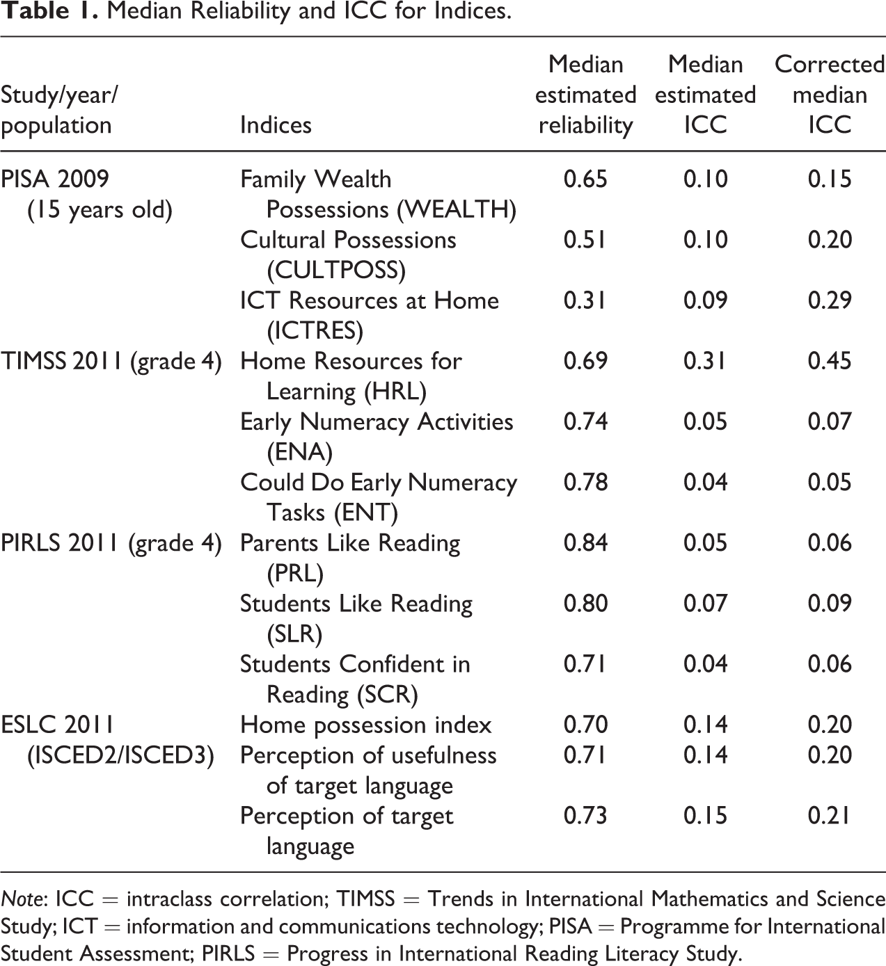
Note: ICC = intraclass correlation; TIMSS = Trends in International Mathematics and Science Study; ICT = information and communications technology; PISA = Programme for International Student Assessment; PIRLS = Progress in International Reading Literacy Study.

Reliability estimates presented in Table 1 are taken from technical reports (for PISA, see OECD 2012; for PIRLS and TIMSS, see Mullis et al. 2012; for ESLC, see European Commission 2012), while ICC coefficients were computed by the author. Students’ classroom was a grouping variable in case of PIRLS and TIMSS research, while students’ school was a grouping variable for PISA and ESLC (the grouping variable was dictated by sampling scheme). ICC was estimated using the classical approach (no correction for measurement error was taken into account) in addition, the last column in Table 1 presents naive-corrected ICC (median estimated ICC was divided by estimated reliability) just to show approximately the true scale of phenomena that might appear in the data.

Juxtaposing simulation results with example data provided in Table 1 shows that using a simple multilevel model for compositional analysis on large-scale assessment data might bring serious biases in real-data situations. Let’s look, for instance, at cultural possession (CULTPOSS) in PISA data. Assuming that compositional effect is not present (equals zero in population) and individual effect is moderate (equals .4 for standardized variable), having median country in terms of reliability and ICC, we would guess that biases would be significant for both individual and compositional effect. On examining Figure 1, we would expect that estimates (in unstandardized metric) might even cross, that is, the estimate of compositional effect would be greater than the individual effect. If we look at Information and Communications Technology Resources at Home in PISA or Home Resources for Learning (HRL), biases might be even greater. Other examples are less striking, but nevertheless for median country and individual effect of 0.4 or greater, we could expect potentially troublesome biases.

Solutions

In this section, some solutions for problems discussed earlier are provided. This article focuses on a situation where the researcher is dealing with composite measures, that is, measures constructed from several questions. This scenario often happens in survey applications when the respondent is asked a battery of questions concerning the same construct (social status, well-being, psychological constructs, etc.). This will be shown in two of the three proposed solutions, namely using plausible values (PVs) methodology for independent variables and SEM with multilevel item response theory (IRT) measurement structure—namely, the doubly latent (DL) model.

In other circumstances, where the researcher does not deal with constructed measures, one solution is provided—namely, correction for estimates of multilevel model using classical measurement error assumptions. The requirements of this method are that information about the reliability and estimate of ICC are needed. Reliability is sometimes hard to estimate, but some possibilities do exist (Ashenfelter and Krueger 1994; Longford 1993).

In the following section, three proposed methods are briefly described. Then, in the next section, results from simulation studies assessing performance of those methods are presented.

Multilevel Model With Analytical Correction

The analytical approach is based on corrections of fixed effects and obtained from a simple multilevel model. The correction was made using derivations presented in Maddala (1986:447)

p l i m {\hat{γ}}_{10} = γ_{10} - \frac{γ_{10} (1 - α_{10}) - ρ γ_{01} (1 - α_{01})}{1 - ρ^{2}}

p l i m {\hat{γ}}_{01} = γ_{01} - \frac{γ_{01} (1 - α_{01}) - ρ γ_{10} (1 - α_{10})}{1 - ρ^{2}}

(where ρ² = ICC)

Equations (10) and (11) are similar to equations (7) and (8) presented earlier except that α₁₀ is introduced as the reliability of compositional variable and α₀₁ is the reliability of individual variable. Based on those derivations, a system of equations was introduced as parameter constrains added to the simple multilevel model:

{\hat{γ}}_{10}^{C} = \frac{({\hat{ρ}}^{2} - 1) {\hat{γ}}_{10}^{M L} + \hat{ρ} (1 - {\hat{α}}_{01}) {\hat{γ}}_{01}^{C}}{(1 - {\hat{α}}_{10}) + {\hat{ρ}}^{2} - 1},

{\hat{γ}}_{01}^{C} = \frac{({\hat{ρ}}^{2} - 1) {\hat{γ}}_{01}^{M L} + \hat{ρ} (1 - {\hat{α}}_{10}) {\hat{γ}}_{10}^{C}}{(1 - {\hat{α}}_{01}) + {\hat{ρ}}^{2} - 1},

where parameters indexed with letter C denote corrected estimates and parameters indexed with ML denote uncorrected maximum likelihood estimates for multilevel models. Estimates of ICC and reliability were provided from additional computation. In simulation studies presented later in this article, estimates of reliability were based on Cronbach’s α coefficient and ICC was estimated using multilevel regression. ICC was also corrected by dividing it by Cronbach’s α to adjust for the measurement error problem in ICC estimation.

This solution seems to be not very accurate. First, it is not very likely that classical measurement error assumptions are true for most situations. Second, reliability and ICC are introduced to the estimation as if they would be known when in fact they are estimated separately in the outside step which would affect standard error estimation and might affect quality of correction. Third, correction for attenuation using Cronbach’s α might not be very accurate, because α in most cases underestimates reliability (Schmitt 1996). Nevertheless, this approach is relatively simple to implement and is possible when no data on item levels are available. Neither of the two next approaches have such advantages.

Multilevel Model With PVs

The second approach is based on PVs methodology (for an extended discussion, see Mislevy et al. 1992; Von Davier, Gonzales, and Mislevy 2009). In short, PVs represent random draws from an empirically derived distribution of latent variables that is conditional on the observed values of the scale (measurement model) and the covariates (latent regression):

P (θ_{j} | y_{j}, x_{j}, β, Γ, Σ) \propto P (x_{j} | θ_{j}, β) P (θ_{j} | y_{j}, Γ, Σ),

where θ is the latent variable, β is the matrix of responses (x _j ) parameters, Γ is a matrix of latent regression coefficients for the covariates (y _j ), and Σ is a common variance matrix for residuals.

Parameters and posteriori distribution presented in equation (14) are usually estimated and PVs are drawn using the Markov Chain Monte Carlo methods (see detailed description in Fox and Glas 2001, 2003) in Bayesian estimation framework. When the procedure is finished, a set of PVs is generated, and each respondent receives several indicators (PVs) of latent variable. PVs might be then used in subsequent analysis. Each PV is used once in each analysis. For instance, for five generated PVs, five models are estimated; in each model, one PV is used and the final estimates are obtained using the so-called Rubin’s rule (Little and Rubin 1987)—results from all analyses are simply averaged.

As PVs are random draws, the random component provides a way to model the uncertainty associated with the estimate that is related to the measurement error (Wu 2005). By using PVs instead of raw estimates of student ability, we eliminate the impact of measurement error bias in the independent variable. Moreover, PVs have approximately the same conditional distribution as the latent trait being measured. The latent regression part (i.e., Σ and Γ matrixes) adjusts PVs to have conditional distribution on covariates (taken into account in the generating process) the same as the latent distribution conditioned on covariates, so the results obtained from the PVs are assumed to be close to the results that would be obtained using latent regression modeling (for more details, see Mislevy et al. 1992).

For the analysis presented in this article, PVs were generated for the independent individual variable used in compositional effect modeling. For conditioning (i.e., the latent regression part), two variables were used: (1) the dependent variable used in compositional effect modeling (obtained from IRT modeling) and (2) the mean of independent variables in the group obtained as the group mean of IRT estimate of individual results. Usage of the second variable is the shortcut for using dummy variables for all 100 groups which would be more appropriate but far more computation demanding and impractical in case of large data sets (the less appropriate strategy adopted here was also used in PISA analysis till 2006). In each simulation, five PVs for the independent variable were generated and five models were computed. After that, results were averaged using Rubin’s rule. All computations were made using Mplus 6.11.

DL Model

The last approach is based on a multilevel SEM with latent aggregation structure: the DL model (Marsh et al. 2009). The DL model is based on multilevel structural equating modeling where the structural part of the equation may be written as multilevel regression with latent predictors (θ _xij –individual latent variable; θ _xj —compositional latent variable; u_0j—stays for level-2 residuals; and r_ij for level-1 residuals):

y_{i j} = γ_{00} + γ_{10} θ_{i j} + γ_{01} {\overset{ˉ}{θ}}_{j} + u_{0 j} + r_{i j},

the measurement part on individual level:

P (x_{k i j} = 1 | θ_{i j}) = l o g i t (μ_{k} + λ_{k, W} θ_{i j}); k = 1, \dots, K,

and the measurement part on group level:

{\overset{ˉ}{x}}_{k j} = μ_{k} + λ_{k, M} {\overset{ˉ}{θ}}_{j}; k = 1, \dots, K .

On individual-level measurement model (16),³ the probability of a correct response for item k, for respondent i in group j is modeled by confirmatory factor model with within-factor loadings (λ _k , _W ) and item intercepts (μ _k )—discrimination and difficulty parameters in IRT. On group level (17), aggregate responses ( ${\overset{ˉ}{x}}_{k j}$ ) are modeled by factor model with between-factor loadings ( $λ_{k x, M}$ ) and shared with level-1 item intercepts (μ _k ).

A graphical representation of the equations described previously is shown in Figure 5. In the DL model, latent variables are specified on both levels: individual and group. The measurement part of the group-level model reflects the measurement part on the individual level with equality constraints on each pair within- and between-factor loadings (λ _k _,W = λ _k _,B for any k). Using this parameterization, the DL model takes into account measurement error for both individual- and group-level variables in the same way that the one-level structural equating model takes into account measurement error of individual variables. Additionally, this model also accounts for sampling errors introduced by complex sampling where only some students are sampled from analyzed groups. The model does not come without some drawbacks. As opposed to other models, DL model centered on groups is required for identification purposes, and the compositional effect must be obtained as the difference of between and within effects (for details, see Marsh et al. 2009). Equality constraints across loadings introduce an additional assumption that the compositional effect reflects exactly the process taking place on the individual level and this might not always be plausible. In addition, the model is relatively demanding with respect to computing. It might be estimated using ML techniques; however, no closed formulas for likelihood functions are known, and numerical integration must be introduced to estimate the desired parameter (for detailed description of the DL model and discussion of its assumptions, see Marsh and Hau 2003; Marsh et al. 2009). In fact, for simulations presented in this article, DL appears to be more time consuming and computationally demanding than Bayesian estimation of PVs.

Figure 5.

Graphical representation of doubly latent model.

Evaluation

Monte Carlo simulation studies were conducted to assess the performance of the proposed solutions. As in previously presented simulations, artificial data with known structure were generated. The following algorithm for data sets preparation was used, in each simulation:

100 groups with 30 individuals in each group were sampled from the true population model where compositional effect equals 0; the individual effect equals 0.4 (variant 1) or 0.7 (variant 2) and ICC equals 0.2. Y as well as X variables were set to have mean 0 and standard deviation 1. The variables Y and X reflect latent variables.

To introduce measurement error for each respondent, 20 binary responses were generated according to a two-parameter logistic model (Birnbaum 1968) both for Y and X. For each simulated data set, difficulty parameters were sampled from standard normal distribution, and discrimination parameters were sampled from normal distribution where means differ from sample to sample to achieve a uniform range of reliabilities bounded between .2 and .85.

In total, 30,000 simulated data sets for each scenario were generated. As in previously presented simulations, it is also assumed here that entire groups are sampled, not just a random samples of students from each group. A classical multilevel model, a multilevel model with analytical correction, a model with PVs, and an SEM with latent aggregation (DL model) were tested using generated data. All models were estimated using Mplus 6.11 software.

Figure 6 shows how the different methods recover the individual effects. In both scenarios (when the individual effect is high: .7; or moderate .4), parameter estimates from the multilevel model with PVs are practically unbiased (with little tendency for overestimating the effect) even when reliability is extremely low. Estimates based on the DL model are almost as good as estimates based on PVs when the individual effect is moderate (with little tendency for underestimating the effect). Small but consistent underestimation of the individual effect might be found when the individual effect is high. Both classical multilevel model and corrected multilevel model are highly biased; the first model underestimates individual effect, while the latter overestimates it. The bias grows when reliability decreases. Both multilevel model and corrected multilevel model seem to provide reasonable approximation of individual effects when reliability is relatively high.

Figure 6.

Parameter estimates for individual effects when true individual equals .7 (upper panel) and true individual equals .4 (lower panel). Different methods. Based on 30,000 simulated data sets with varying reliability of independent variable, ICC = .2. Note: ICC = intraclass correlation.

Figure 7 is similar to Figure 6 but gives results for compositional effect estimates instead of individual effects. In this case, the DL model performs best with virtually unbiased results. The PVs methodology gives very good results when the individual effect is moderate even with moderate reliability (but higher than .65). The performance of the multilevel model based on PVs methodology is slightly worse, showing underestimation when individual effects are high (while still giving reasonably good estimates with reliability higher than .7). The performance of the corrected multilevel model is worse than the model with PVs and DL model, but still significantly better than the simple multilevel model.

Figure 7.

Parameter estimates for compositional effects when true individual equals .7 (upper panel) and true individual equals .4 (lower panel). Different methods. Based on 30,000 simulated data sets with different reliability of independent variable, ICC = .2. Note: ICC = intraclass correlation.

While Figures 6 and 7 show the quality of point estimates based on different models. Figure 8 presents the quality of inferences based on each model. The bars on the graphs presented in Figure 8 represent the percentage of estimates significantly different from the true compositional effect (p < .05). While the compositional effects in these simulations were set to be 0, the percentage in the graphs might be interpreted as the probability that the compositional effect will be recognized as significant (p < .05), while in fact it does not exist (under simulation conditions).

Figure 8.

Percentage of rejections of hypothesis states that compositional effects do not differ from 0. Two scenarios when true individual effect equals .7 and .4. Results based on 30,000 simulated data sets with different reliability of independent variable, ICC = .2. Note: ICC = intraclass correlation.

When the individual effect is strong (0.7) with moderate ICC (.2) and reliability smaller than .85, the simple multilevel model in virtually all attempts gives significant results. With moderate individual effect (0.4), the situation is better, but still for a reliability range of .75 to .85, half of the estimates in the simulation study indicate significant compositional effect despite the lack of effect in the simulated data.

All introduced corrections improve inferences on the compositional effect. The overall performance is best in the DL model. In each presented levels of reliability, 20 percent of the estimates give significant compositional effects. This indicates that the DL model underestimates standard errors by 15 percent (using significance testing with p < .05, one would expect 5 percent of significance results for unbiased standard errors). Even if standard errors are overestimated, it should be noticed that DL model gives quite reasonable estimates in extremely low reliability even below .35. This is not the case for any other presented corrections.

The model with PVs performs best with relatively high reliability (greater than .75). In this situation, it gives point estimates almost as good as the DL model does (Figure 7); however, significance testing is more appropriate. For a medium individual effect, the percentage of significant results does not exceed 5 percent, which is the number one would expect for p < .05. The performance of the PVs is worse for a high individual effect but is still better than DL model.

The multilevel model with analytical correction looks least favorable. With individual effect set to be 0.7, it gives about 50 percent wrong inferences. However, when reliability is decent (more than .75) and the individual effect is moderate, the analytical corrected model gives more reasonable inferences compared to the uncorrected model.

Empirical Example

In this section, examples of analysis using previously tested methods are shown. TIMSS 2011 (grade 4) was chosen as the example data set for this exercise. TIMSS measures mathematics and science abilities using both items with multiple choice and open-ended response formats. It measures achievement in mathematics and science of more than 500,000 students from over 60 countries. Along with ability measurement, questionnaires for parents were administered in some participating countries to provide information about students’ background (for more details about TIMSS 2011 research, see Mullis et al. 2012).

Three different countries with different characteristics that might influence estimation of individual and compositional effects were chosen: Hungary, Hong Kong, and Ireland. PVs of mathematics achievements were used as dependent variables in all analysis, while the independent variable was constructed based on five items from the HRL scale. Both variables were standardized to have mean 0 and standard deviation of 1 in each country. The HRL scale’s reliability differs from country to country ranging from .8 in Hungary to .69 in Ireland (measured by Cronbach’s α). So do ICC coefficients of independent variables, which equals .37 in Hungary, .36 in Hong Kong, and .2 in Ireland. Countries’ samples differ in terms of number of students, number of groups, and average group size. While in Hungary and Ireland, whole classes were sampled, in Hong Kong, we have to deal with a school sample (details are shown in Table 2). In the analysis provided in this section, the three-level structure (students, classrooms, and schools) was simplified to a two-level structure: students and classrooms for Hungary and Ireland and students and schools for Hong Kong.

Table 2.

Estimates of Individual and Contextual Effects Math Performance on Home Resources for Learning Using TIMSS 2011 Data.

Individual effects
Method	Hungary		Hong Kong		Ireland
Method	Est.	(SE)	Est.	(SE)	Est.	(SE)
Multilevel	0.406**	(0.020)	0.101**	(0.018)	0.395**	(0.019)
Corrected multilevel	0.587**	(0.029)	0.186**	(0.033)	0.643**	(0.031)
Plausible values	0.548**	(0.018)	0.125**	(0.018)	0.534**	(0.020)
Doubly latent model	0.428**	(0.063)	0.107**	(0.019)	0.459**	(0.023)
Compositional effects
	Hungary		Hong Kong		Ireland
Method	Est.	(SE)	Est.	(SE)	Est.	(SE)
Multilevel	0.371**	(0.095)	0.278**	(0.059)	0.189**	(0.051)
Corrected multilevel	0.226**	(0.044)	0.232**	(0.063)	0.080	(0.054)
Plausible values	0.166**	(0.036)	0.216**	(0.053)	0.051	(0.045)
Doubly latent model	0.128**	(0.033)	0.199**	(0.057)	0.043	(0.048)
Number of students	5,988		6,642		4,204
Number of groups	249		132		220
Average group size	24.048		50.318		19.110
α of HRL	0.804		0.720		0.691
ICC of HRL	0.369		0.357		0.200

Note: SE = standard error; ICC = intraclass correlation; HRC = Home Resources for Learning; TIMSS = Trends in International Mathematics and Science Study.

**p < .01.

Because of the use of PVs (five PVs are available for each measure in TIMSS) five sets of models were fitted, each for every PV; results were combined using the Rubin rule (Little and Rubin 1987). For instance, five DL models were estimated, each one with one PV. Then estimates from the five models were aggregated using the Rubin rule. When PVs methodology was used to generate PVs for independent variables, five computations were also conducted. The model with the first PVs for mathematical achievement (dependent variable) and the first PVs for HRL was estimated. Then the second PVs for mathematical achievement and the second PVs for HRL were used. This procedure was repeated till all five estimations were finished. In the end, results from the five sets of estimates were aggregated.

Table 2 represents results for four different methods for each of the three countries. In the upper part of the table, individual effects are shown, while the lower part of the table shows compositional effect estimates. In the case of Hungary, corrected results and models based on PVs are significantly larger than the simple multilevel model. Estimates from the DL model are characterized by very large standard error and do not differ significantly (p < .05) from other methods. All in all, the four methods give the same conclusion about a strong relation between the individual HRL variable and maths achievements. Results are consistent with simulation studies. The simple multilevel model and DL model give smaller estimates than PVs (most reliable in estimating individual effects according to simulations), while corrected multilevel shows a stronger effect. In the case of Hong Kong, the conclusions are the same—a small but significant relation was found. In Hungary, the multilevel model and DL model give smaller values for the effect than PVs, while the corrected multilevel model gives larger values; however, in this case, the result for the corrected model is relatively big compared to other results. Results for the corrected multilevel model are not surprising because the reliability coefficient of HRL is relatively low and simulated results show the corrected multilevel model is very sensitive to the decrease in reliability. Results for Ireland seem to show the same pattern as for the two previously mentioned countries.

Results for compositional effects estimation show greater variability than individual effects estimates. In the case of Hungary, the simple multilevel method indicates a relatively high compositional effect, while corrected results show a rather small effect. Additionally, results go along with results of the simulation study. The DL model and PVs models provide similar small effects, the estimate from the multilevel model is highest, and the corrected multilevel technique gives results in between. In Hong Kong, sample results are similar; however, differences between estimates are relatively small. Ireland is most interesting because depending on whether the researcher uses corrected methods or not, different conclusions can be drawn. Using the uncorrected multilevel model, one would infer a significant contextual level, while using models accounting for low reliability leads to an insignificant compositional effect.

Summary and Discussion

The article shows that reliability might be an important issue in compositional effects estimation. Not taking it into account might bring statistical artifacts that might fool the researcher’s attempts to reveal the studied problems. Three propositions for corrections were introduced, all of which improve the quality of inferences. The overall performance of the DL model suggests that it would be the most preferable method in most conditions, especially when reliability is relatively low. However, the model with PVs might be preferable when the reliability of independent variables is relatively high. With reliabilities as high as .8, the model with PVs gives almost as good point estimates as the DL model, but more appropriate standard errors. When dependent variables are not constructed using several items but are other kinds of indicators (with measurement error), analytical correction might make an important contribution to reducing biases and improving the quality of inference. One should keep in mind that analytical corrections work satisfactorily for relatively high reliability (more than .8) only.

In the light of the good performance of the multilevel model using the PVs methodology, it might be worth considering introducing the PVs methodology in scaling indices in programs that deal with multilevel structure of data. For instance, while PVs models are widely used in scaling cognitive indices (for instance, math achievements in TIMSS, reading achievements in PIRS, etc.), other indices (see Table 1 for examples) are constructed without PV methodology. It was shown that introducing PVs methodology for those indices might be beneficial for at least compositional effect estimation and most probably for single-level models as well.

This article does not cover all topics that might be connected with measurement error. For instance, no measurement error on the dependent variable was assumed. Only continuous outcomes were investigated and it might be very interesting to see how models for categorical data cope with imperfect reliability. No consideration for group size and potential sampling processes inside groups was made. Finally, very simple models without any additional control variables (that might account for ICC) and models without random slopes were tested. All these things should be investigated in future studies. This study shows the general problem and some basic solutions focusing on simple mechanisms to examine them properly. However, in more complex situations, it is very unlikely that the general direction of bias and general conclusions from this study would differ.

Footnotes

Appendix

Declaration of Conflicting Interests

The author(s) declared no potential conflicts of interest with respect to the research, authorship, and/or publication of this article.

Funding

The author(s) disclosed receipt of the following financial support for the research, authorship, and/or publication of this article: This work was partially supported by the internal research grant of Educational Research Institute, Warsaw.

Notes

References

Ashenfelter

Orley

Krueger

Alan B.

. 1994. “Estimates of the Economic Returns to Schooling from a New Sample of Twins.” American Economic Review 84:1157–73.

Birnbaum

1968. “Some Latent Trait Models and Their Use in Inferring an Examinee's Ability.” Pp. 374–472 in Statistical Theories of Mental Scores, edited by Lord

F. M.

Novick

M. R.

, chap. 17-20. Reading, MA: Addison-Wesley.

Bowling

2005. “Mode of Questionnaire Administration Can Have Serious Effects on Data Quality.” Journal of Public Health 27:281–91.

Dedrick

R. F.

Ferron

J. M.

Hess

M. R.

Hogarty

K. Y.

Kromrey

J. D.

Lang

T. R.

Lee

R. S.

. 2009. “Multilevel Modelling: A Review of Methodological Issues and Applications.” Review of Educational Research 79:69–102.

Degracie

J. S.

Fuller

W. A.

. 1972. “Estimation of the Slope and Analysis of Covariance When the Concomitant Variable Is Measured with Error.” Journal of the American Statistical Association 67:930–37.

European Commission. 2012. First European Survey on Language Competences: Technical Report. European Union. Accessed July 9, 2013, http://ec.europa.eu/languages/eslc/docs/en/technical-report-eslc_en.pdf.

Fox

J. P.

Glas

C. A. W.

. 2001. “Bayesian Estimation of a Multi-level IRT Model Using Gibbs Sampling.” Psychometrika 66:271–88.

Fox

J. P.

Glas

C. A. W.

. 2003. “Bayesian Modeling of Measurement Error in Predictor Variables.” Psychometrika 68:169–91.

Fuller

W. A

. 1987. Measurement Error Models. Vol. 305. New York: John Wiley.

10.

Gronlund

N. E

. 1998. Assessment of Student Achievement. Needham Heights, MA: Allyn & Bacon Publishing.

11.

Harker

Tymms

. 2004. “The Effects of Student Composition on School Outcomes.” School Effectiveness and School Improvement 15:177–99.

12.

Hox

2010. Multilevel Analysis: Techniques and Applications. London, UK: Routledge Academic.

13.

Kim

J. S.

Frees

E. W.

. 2006. “Omitted Variables in Multilevel Models.” Psychometrika 71:659–90.

14.

Little

R. J. A.

Rubin

D. B.

. 1987. Statistical Analysis with Missing Data. New York: John Wiley.

15.

Longford

N. T.

1993. “Regression Analysis of Multilevel Data with Measurement Error.” British Journal of Mathematical and Statistical Psychology 46:301–11.

16.

Maas

C. J.

Hox

J. J.

. 2004. “The Influence of Violations of Assumptions on Multilevel Parameter Estimates and Their Standard Errors.” Computational Statistics & Data Analysis 46:427–40.

17.

Madansky

1959. “The Fitting of Straight Lines When Both Variables Are Subject to Error.” Journal of the American Statistical Association 54:173–205.

18.

Maddala

G. S.

1986. Limited-dependent and Qualitative Variables in Econometrics. Cambridge, UK: Cambridge University Press.

19.

Maddala

G. S.

1992. Introduction to Econometrics. Englewood Cliffs, NJ: Prentice Hall.

20.

Marsh

H. W.

Hau

K. T.

. 2003. “Big-fish-little-pond Effect on Academic Self-concept.” American Psychologist 58:364–76.

21.

Marsh

H. W.

Lüdtke

Robitzsch

Trautwein

Asparouhov

Muthén

Nagengast

. 2009. “Doubly-latent Models of School Contextual Effects: Integrating Multilevel and Structural Equation Approaches to Control Measurement and Sampling Error.” Multivariate Behavioral Research 44:764–802.

22.

Mislevy

R. J.

Beaton

A. E.

Kaplan

Sheehan

K. M.

. 1992. “Estimating Population Characteristics from Sparse Matrix Samples of Item Responses.” Journal of Educational Measurement 29:133–61.

23.

Morton-Jones

Henderson

. 2000. “Generalized Least Squares with Ignored Errors in Variables.” Technometrics 42:366–75.

24.

Mullis

I. V. S.

Martin

M. O.

Foy

Drucker

K. T.

. 2012. TIMSS 2011 International results in mathematics. Chestnut Hill, MA: TIMSS & PIRLS International Study Center, Boston College.

25.

OECD (Organization for Economic Cooperation and Development). 2007. PISA 2006: Science Competencies for Tomorrow's World: Volume 1: Analysis. OECD Publishing.

26.

OECD (Organization for Economic Cooperation and Development). 2012. PISA 2009. Technical Report. Paris, France: OECD Publishing.

27.

Raudenbush

S. W.

Bryk

A. S.

. 2002. Hierarchical Linear Models: Applications and Data Analysis Methods. Vol. 1. Thousand Oaks, CA: Sage.

28.

Scheerens

Glas

C. A.

Thomas

S. M.

Thomas

. 2003. Educational Evaluation, Assessment, and Monitoring: A Systemic Approach. Bristol, UK: Taylor & Francis.

29.

Schmitt

1996. “Uses and Abuses of Coefficient Alpha.” Psychological Assessment 8:350.

30.

Shear

B. R.

Zumbo

B. D.

. 2013. “False Positives in Multiple Regression Unanticipated Consequences of Measurement Error in the Predictor Variables.” Educational and Psychological Measurement 73:733–56.

31.

Snijders

T. A.

Bosker

R. J.

. 1999. Multilevel Analysis: An Introduction to Basic and Advanced Multilevel Modelling. London, UK: Sage.

32.

Thomas

Mortimore

. 1996. “Comparison of Value-added Models for Secondary-school Effectiveness.” Research Papers in Education 11:5–33.

33.

Tymms

P. B

. 1992. “The Relative Effectiveness of Post-16 Institutions in England (Including Assisted Places Scheme Schools).” British Educational Research Journal 18:175–92.

34.

Wolf

L. F.

Smith

J. K.

Birnbaum

M. E.

. 1995. “Consequence of Performance, Test, Motivation, and Mentally Taxing Items.” Applied Measurement in Education 8:341–51.

35.

Woodhouse

Yang

Goldstein

Rasbash

. 1996. “Adjusting for Measurement Error in Multilevel Analysis.” Journal of the Royal Statistical Society. Series A (Statistics in Society) 159:201–12.

36.

(2005). The role of plausible values in large-scale surveys. Studies in Educational Evaluation 31:114–28.

37.

Von Davier

Matthias

Gonzalez

Mislevy

. 2009. “What Are Plausible Values and Why Are They Useful.” IERI Monograph Series 2:9–36.

38.

Yuan

K. H.

Bentler

P. M.

. 2004. “On the Asymptotic Distributions of Two Statistics for Two-level Covariance Structure Models within the Class of Elliptical Distributions.” Psychometrika 69:437–57.