
Abstract
In its standard formulation, sequence analysis aims at finding typical patterns in a set of life courses represented as sequences. Recently, some proposals have been introduced to jointly analyze sequences defined on different domains (e.g., work career, partnership, and parental histories). We introduce measures to evaluate whether a set of domains are interrelated and their joint analysis justified. Also, we discuss about the quality of the results obtained using joint sequence analysis. In particular, we focus on cluster analysis and propose criteria to assess whether clusters obtained using a joint approach satisfactorily describe each domain.
Keywords
Introduction and Motivation
Sequence analysis (SA) is now an established technique to describe life course trajectories (see Aisenbrey and Fasang 2010; Elzinga 2003, 2007, for a discussion). The aim of SA is to describe life courses represented as sequences, that is, the ordered collections of the states (activities) experienced by individuals during a period of time. A major issue in SA concerns the identification of the most typical patterns in data, and the identification of individuals who experienced similar trajectories. Therefore, the proper measurement of the dissimilarity between two trajectories plays a crucial role in SA. Actually, optimal matching analysis (OMA), introduced in the social sciences by Abbott and Forrest (1986) to calculate and analyze pair-wise dissimilarities between sequences “has become the standard technique so much that sequence analysis and OMA-like techniques are commonly regarded as being almost synonymous” (Elzinga 2003).
In its “standard” formulation, SA focuses on life courses defined on a single domain. Examples concern the analysis of early careers, work careers, and retirement patterns (Abbott and Hrychak 1990; Blair-Loy 1999; Chan 1994, 1995; Han and Moen 1999a; Malo and Munoz-Bùllon 2003; McVicar and Anyadike-Danes 2001; Scherer 2001; Schoon et al. 2001; Stovel, Savage, and Bearman 1996), of social mobility (Halpin and Chan 1998), of housing and residential mobility (Clark, Deurloo, and Dieleman 2003; Stovel and Bolan 2004), and of family formation (Aassve, Billari, and Piccarreta 2007; Piccarreta and Billari 2007).
Nonetheless, often social scientists are interested to study several domains, which are supposedly related one to another. Relevant examples are the joint analysis of the work, family, and housing trajectories, or of the work or family formation histories of parents and of their children.
Some proposals along this direction are described and discussed in the second section. Han and Moen (1999b) and Widmer and Ritschard (2009) propose to preliminarily simplify the domains using separate cluster analyses and to study the relation between the obtained results. Other approaches are instead focused on the definition of joint dissimilarities combining information on the domains. Aassve et al. (2007) and Piccarreta and Billari (2007) suggest to build a trajectory describing the combination of states experienced in each period. Pollock (2007) and Gauthier et al. (2010) introduce multiple sequence analysis (MSA), a technique to compute optimal matching (OM) distances based on sequences defined on the different domains.
A joint analysis can serve both to explore the relations among domains and to exploit such relations to obtain joint rather than marginal results. The above mentioned proposals are mostly focused on the latter aspect. However, surely a joint analysis of domains is worth, reasonable, and effective when the domains are associated.
For the case of two domains, Piccarreta and Lior (2010) propose a graphical approach to visualize their relation, and Piccarreta and Elzinga (2013) introduce criteria to quantify the strength of the possible association.
In this article, we focus on the relations among several domains and extend the work of Piccarreta and Elzinga (2013) following two main directions.
First, in the third section we consider the association between domains. Concepts very popular in multivariate data analysis, namely, Cronbach’s α and principal components analysis (PCA), are extended to our context to explore the relations among the domains prior to the possible application of a joint analysis. We then consider the relation between joint and domain-specific dissimilarities, to evaluate if and to what extent the former can be used without losing relevant information on one or more domains.
Second, we consider the problem of assessing the performance of joint dissimilarities when employed in the dissimilarities-based procedures solely applied in SA, such as cluster analysis (CA), multidimensional scaling, analysis of variance (ANOVA), or regression trees. While comparing the results obtained using joint and domain-specific dissimilarities is surely a relevant issue, suitable criteria at this aim necessarily differ from one technique to another.
For the sake of synthesis, in the fourth section, we limit attention to CA, one of the most popular techniques in SA (actually, all the abovementioned contributions on the joint analysis of domains refer to CA). Also, CA unveils the most relevant patterns in data, and it can be used in our context to visualize the most relevant combinations of the domains’ trajectories. Finally, as it will be discussed later, some conclusions on the domains’ interrelations can also be drawn based on the results of CA.
Our proposals are analyzed referring first to synthetic data, and then, in the fifth section, to data arising from the British Household Panel Survey, already used in Pollock (2007).
“Simple” and Joint Sequence Analysis (JSA): A Brief Overview
SA usually focuses on the description of life courses defined on a single life domain (e.g., education, family formation, work career). The observed individuals’ trajectories are represented by sequences, that is, ordered collection of the states experienced during a given period. For a given domain D, the set of the possible states that can be observed in each period, Ω D , is called alphabet. Thus, sequences are categorical time series whose elements are included in Ω D.
The application of SA to the analysis of life courses traces back to the work of Andrew Abbott and his coauthors (Abbott 1990a, 1990b, 1995; Abbott and Forrest 1986; Abbott and Hrychak 1990). In their seminal paper, Abbott and Forrest (1986) extended to sociology the work of Sankoff and Kruskal (1983), who used OM (originated in the field of information theory and computer science; Hamming 1950; Levenshtein 1966) to study DNA sequences.
OM
1
is an aligning technique used to measure the dissimilarity between two sequences taking into account the duration and possible simultaneity of events. Such dissimilarity is based on the operations needed to transform one sequence into another. Three operations are considered: insertion (of a state into the sequence), deletion (of a state from the sequence), and substitution (of one state with another). A cost is assigned to each operation, ideally reflecting the difficulty of modifying a sequence according to the operation itself. If K operations, o
1, …, oK, are needed to transform the ith sequence into the hth one (or conversely), the total transformation cost is determined as the sum of the single operation costs,
A heated debate in the literature concerns the choice of costs (see, e.g., Elzinga 2003; Halpin 2003), and a number of proposals have been introduced partially modifying the original algorithm (see among others, Gauthier et al. 2009; Halpin 2010; Hollister 2009; Lesnard 2010; MacIndoe and Abbott 2004). Also, measures of dissimilarity alternative to OM have been introduced (Elzinga 2003, 2007). Each proposal has its pros and cons, but standard OM surely remains the approach most used in social sciences (Aisenbrey and Fasang 2010).
In its “standard” formulation, SA focuses on life courses defined on a single domain. In many applications, limiting attention to a single domain might be reductive, and it can be of interest to study the interplay between several domains (i.e., trajectories describing different careers—e.g., work, family, housing), possibly related one to another.
A first way to do so is to evaluate the association between the results obtained for each domain. This approach has been usually adopted when only two domains are taken into account. In Han and Moen (1999b), CA is applied to the two domains separately, and the association between the two obtained partitions is analyzed. Of course, this is reasonable only when the domain-specific clusters are highly homogeneous. Also, problems can arise when more than two domains are considered 2 (multiple contingency tables should be analyzed, possibly with multiple correspondence analysis). More importantly, no attempt is done to combine domains’ characteristics.
In general terms, with JSA of two or more domains, we refer to any approach leading to the definition of joint dissimilarities based on the information arising from all the domains taken into account.
Along this line, some authors (see among the others, Aassve et al. 2007; Lesnard 2008; Piccarreta and Billari 2007) suggest building a combined domain, describing the combination of states experienced in each period. Even if in the context of life course analysis the number of domains analyzed jointly will generally be limited, the combined sequences can easily turn out to be noisy and unstable. Therefore, this approach is reasonable and convenient only when few, connected domains are considered, so that the number of states of the combined alphabet is not too high.
Another possibility is to combine (by averaging or summation) the domain-specific dissimilarities. This clearly resembles what is done for numerical vectors: For example, the squared Euclidean distance for a vector of measurements is the sum of the squared Euclidean distances component by component. This permits to easily combine domains without losing information on their complexity, as measured by the domain-specific dissimilarities. Nonetheless, this approach disregards the cost needed to simultaneously align the set of sequences (one for each domain) characterizing one individual with the set of sequences characterizing another.
This is what is done combining the costs defined for the specific domains. This idea (Blair-Loy 1999; Stovel et al. 1996), formalized and systematized by Pollock (2007) and Gauthier et al. (2010), consists in calculating the dissimilarity between two cases by averaging the substitutions (and insertion and deletion) costs needed to align the sequences in each domain. This approach, named MSA (Pollock 2007), nicely extends the rationale underlying OM to the case of multiple domains. Also, it preserves the information on each domain, as measured by the specific transformations costs. Nonetheless, it is important to observe that MSA, differently from the approaches described earlier, can be only applied when the dissimilarity measure is based on substitution costs (e.g., when OM distance is considered).
While a JSA can be reasonable and well motivated from an interpretative point of view, its implementation is justified and effective only when the considered domains are associated. Also, even in the case of association, joint dissimilarities do not necessarily describe all the domains adequately.
Furthermore, when joint dissimilarities are used in dissimilarities-based procedures (such as, e.g., CA or multidimensional scaling), it is important to assess whether or not the obtained results are satisfactory for all the domains. Clearly, for a given domain, a JSA procedure will possibly perform worse than a domain-specific procedure. Nonetheless, it is important to evaluate whether the loss is homogeneous across domains or if some domains strongly influence the results at the expenses of the others. It is therefore important to assess the extent to which the joint results are actually “joint.”
These aspects are only marginally accounted for in the cited contributions on multiple domains. Actually, most of these works (e.g., Aassve et al. 2007; Han and Moen 1999b; Piccarreta and Billari 2007; Pollock 2007) focus on joint CA and on the substantive interpretation of the obtained clusters. For the case when two domains are considered, Gauthier et al. (2010) discuss the problem and claim that only associated domains should be analyzed jointly, but do not illustrate how to diagnose association in the case of several domains.
In this work, we deal with the mentioned issues. Our aim is first to introduce criteria to evaluate association among domains and second to evaluate if and to what extent a chosen JSA approach is satisfactory with respect to all the domains taken into account.
It is important to underline that our procedures are defined conditionally both to the method chosen to measure domain-specific dissimilarities (e.g., OM) and to the chosen JSA approach. For the sake of illustration, in the following, we will focus, respectively, on OM and MSA (Pollock 2007). The same techniques can be applied also to evaluate other JSA methods. In this sense, our proposals might also be used to compare results obtained using different JSA approaches, but here we consider this as a secondary issue.
Evaluating the Association Among Domains
To evaluate the extent of association between several domains, we extend to our context concepts that are very well known in multivariate data analysis: Cronbach’s α (Cronbach 1951) and PCA (see, e.g., Jolliffe 2002).
To do so, it is necessary to introduce a measure of association or, better, correlation, between two domains. Piccarreta and Elzinga (2013) discuss different indices. Here, we refer to the Mantel coefficient (Mantel 1967), often used in ecology (see, e.g., Legendre and Legendre 1998; Manly 1997). Let
When P domains are considered, P dissimilarity matrices can be built,
To avoid the units of measurement or the ranges of the variables to influence the value of α, standardized variables are usually taken into account, so that σΣ = P (the sum of the P unit variances). In this case, σ
T
coincides with σΣ plus all the pair-wise correlations. If the
To analyze more in detail the relations among the
An alternative measure of association (named JSA association) can be defined by considering the relations between joint and domain-specific dissimilarities. Let
To evaluate JSA association, that is, the adequacy of the (chosen) JSA with respect to the domains, we refer to the Mantel’s coefficients between
Insights on the relations between one domain, say the pth domain, and the others also arise from the analysis of the correlation between
Before proceeding, it is worth to discuss more about the type of association between domains studied using measures of linear (or monotone) association between their dissimilarities. A positive (Mantel’s) coefficient between two sets of dissimilarities is observed when (a) cases similar in one domain are also similar in the other one, (b) cases dissimilar on one domain are also dissimilar on the other one, and (c) the dissimilarities in the two domains increase together.
A negative correlation indicates instead that cases similar on one domain tend to be dissimilar on the other one, and vice versa. Thus, as the dissimilarity between two cases in one domain increases that in the other domain decreases accordingly (in the most extreme situation, two cases will be close in one domain if and only if they are far in the other). This is rarely observed in applications where domains are considered being at least theoretically related.
Focusing on positive correlations, condition (a) must clearly hold to make a joint analysis meaningful. Instead, in some situations, a one-to-many association can exist between domains, so that condition (b) does not hold. For example, people have children irrespective of their marital or occupational status. Also, condition (c) does not refer to the association between domains but, rather, to the relation between the specific domains’ states and dissimilarities. Imagine, for example, an oversimplified society where employed people live in rented houses, self-employed own their houses with a mortgage, and retired own their houses. Employed and self-employed will be the “closest” states in the employment domain, but they will be dissimilar in the housing domain, where owners will be considered as more similar instead. Even if there is clearly an association between these two simplified domains, the corresponding sets of dissimilarities will not be (strongly) linearly related due to the effect of the (chosen) substitution costs (we will refer to the situation when the chosen substitution costs partially mask the association between domains as measured by the correlation between dissimilarities as costs misalignment).
To analyze the behavior of the proposed measures, we simulated six sets of data on five domains characterized by different types and levels of association (Figure 1). In each simulation, five groups of sequences are built for each domain. Individual sequences in each group are characterized by the same combination of experienced states but by slightly different durations (realizations of multinomial random variables).
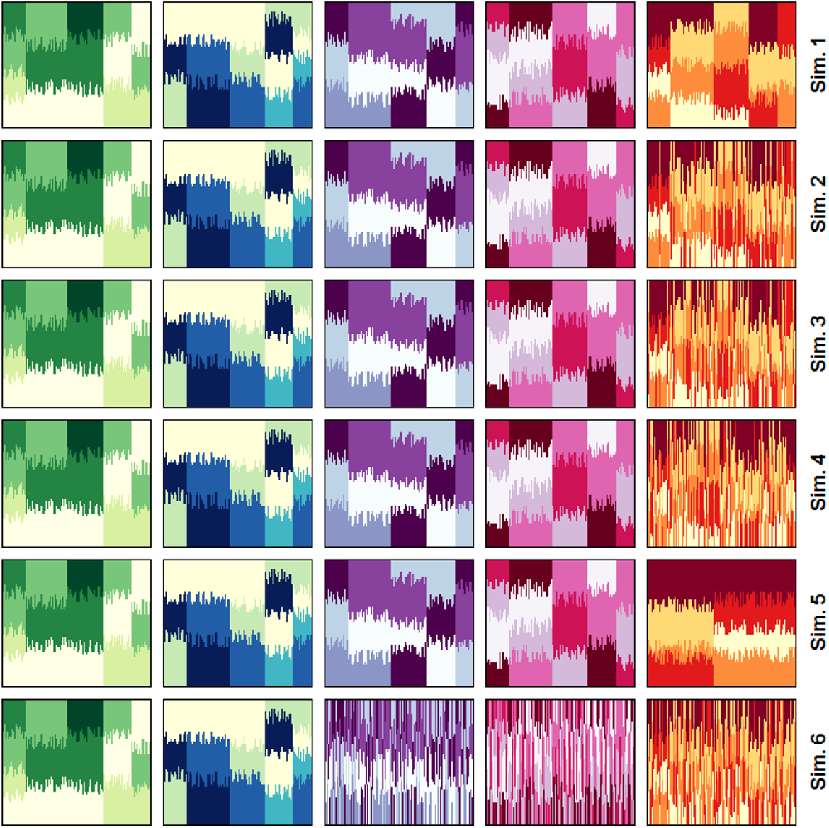
Randomly generated domains with different types and levels of association. Simulation 1: perfect one-to-one matches (PM); Simulations 2 to 4: PM with perturbed fifth domain (30, 50, and 80 percent of sequences randomly permuted). Simulation 5: PM with one-to-many matches for the fifth domain; Simulation 6: Independent blocks (domains 1, 2 and domains 3, 4, and 5) with internally matching domains. Each row reports the five domains for the corresponding simulation. Cases are placed on the horizontal axis, and to each case a vertical bar is associated describing the states experienced during the considered period of time (on the vertical axis), distinguished using different colors. For each simulation, the ordering of cases along the horizontal axis is the same for all the domains.
In simulation 1 (Figure 1, first row), data were generated so that there is a perfect match (PM) between sequences in the different domains: Cases similar in one domain are also similar in the others (thus, condition (a) is satisfied). No adjustments were done to assure that condition (c) holds: Thus, there is not necessarily a perfect linear relation between the domains’ dissimilarities. Even so, since condition (a) holds, we expect our criteria to detect a relevant association (thus, condition (a), when met, should ideally more than compensate the lack of monotone relation between dissimilarities).
In the next simulations, the domains in simulation 1 are modified to build scenarios with different types of association. In simulations 2 to 4 (Figure 1, rows 2–4), a proportion π (30, 50, and 80 percent, respectively) of the sequences in the fifth domain was randomly permuted, thus disrupting the perfect matching of this domain with the others. In simulation 5 (Figure 1, row 5), the fifth domain was simplified, and only two types of sequences were generated, presenting therefore one-to-many matches with sequences in the other domains (thus, condition (b) is not satisfied). Finally, in simulation 6 (Figure 1, row 6), the domains built in simulation 1 were split into two blocks. Domains 1 and 2 (first block) were left unchanged, whereas cases in domains 3 to 5 (second block) were jointly randomly permuted. Hence, the domains in the two blocks remain internally related (one-to-one matches), but the two blocks are not related (sequences in the first block are randomly associated with sequences in the second block). Note that this is the case of lowest association considered here, since the maximal number of connected domains is three (second block).
For each simulation, the domain-specific OM dissimilarity matrices were built using insertion and deletion costs equal to 1 and substitution costs inversely related to the frequency of transition (see Rohwer and Pötter 2004). The global Cronbach’s α and the α−p
’s (obtained without considering the pth domain) are reported in Table 1. Table 2 displays the eigenvalues of the Mantel’s correlation matrix and the loadings of the first and the second PCs. Panel A in Table 3 contains the correlations between the domain-based dissimilarities and the joint dissimilarities calculated using MSA (Gauthier et al. 2010; Pollock 2007),
Simulateda Data: Cronbach’s αs Based on Mantel’s Correlations Between Domain-based Dissimilarities.
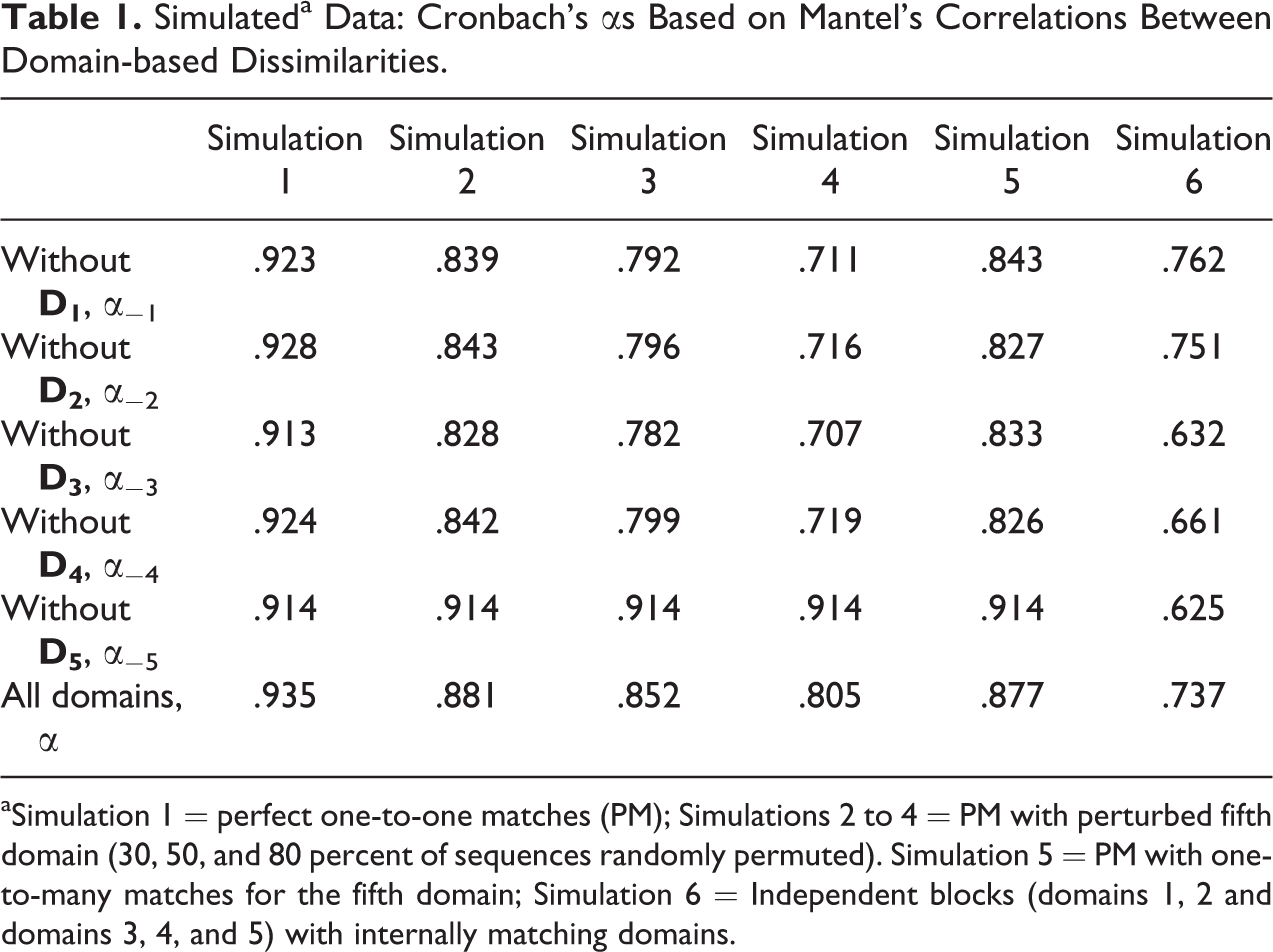
aSimulation 1 = perfect one-to-one matches (PM); Simulations 2 to 4 = PM with perturbed fifth domain (30, 50, and 80 percent of sequences randomly permuted). Simulation 5 = PM with one-to-many matches for the fifth domain; Simulation 6 = Independent blocks (domains 1, 2 and domains 3, 4, and 5) with internally matching domains.
Simulateda Data: Loadings of the First Two PCs (PC1 and PC2) and Eigenvalues (λ1 and λ2) Extracted From the Mantel’s Correlation Matrix Between Domain-based Dissimilarities.
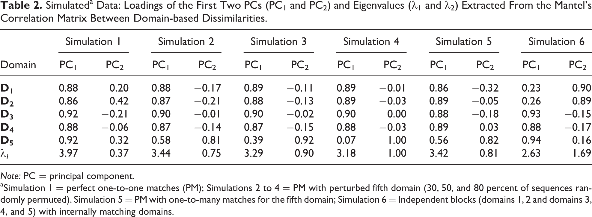
Note: PC = principal component.
aSimulation 1 = perfect one-to-one matches (PM); Simulations 2 to 4 = PM with perturbed fifth domain (30, 50, and 80 percent of sequences randomly permuted). Simulation 5 = PM with one-to-many matches for the fifth domain; Simulation 6 = Independent blocks (domains 1, 2 and domains 3, 4, and 5) with internally matching domains.
Simulateda Data: Mantel’s Correlations Between Domain-based Dissimilarities
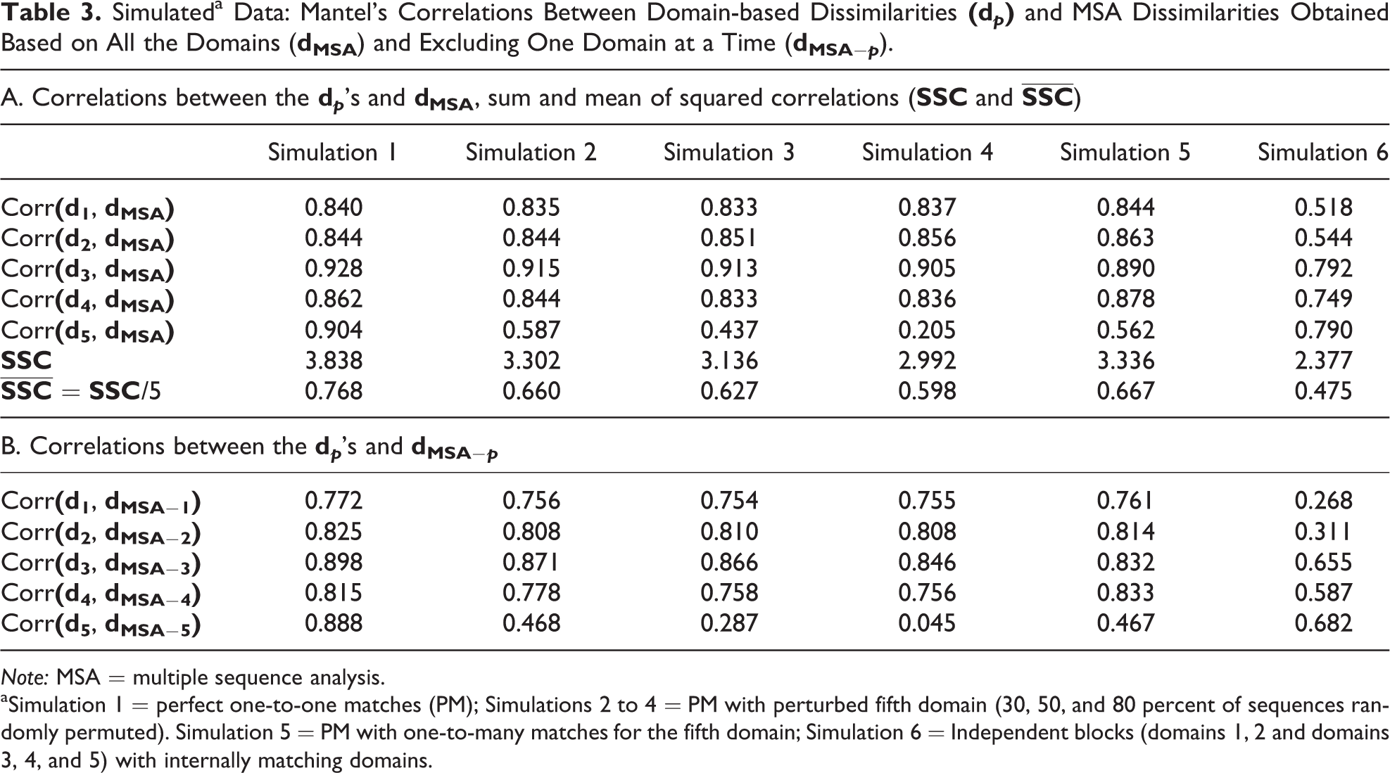
Note: MSA = multiple sequence analysis.
aSimulation 1 = perfect one-to-one matches (PM); Simulations 2 to 4 = PM with perturbed fifth domain (30, 50, and 80 percent of sequences randomly permuted). Simulation 5 = PM with one-to-many matches for the fifth domain; Simulation 6 = Independent blocks (domains 1, 2 and domains 3, 4, and 5) with internally matching domains.
Results in Tables 1–3 reflect the association structure underlying the simulations. For domains in simulation 1, a relevant association is detected. The global α and the first eigenvalue (Tables 1 and 2) are very high, all the domains present high loadings with the first PC, and the α−p
’s are all lower than the global α. Also, the correlations between the
For simulations 2–4, a weaker and weaker association of the fifth domain with the others is correctly diagnosed. The global αs, all lower compared to simulation 1, decrease with the proportion (π) of perturbed sequences, and the deletion of the fifth domain leads to α−5 < α. The second eigenvalues of the Mantel’s correlations matrix and the loadings of the fifth domains on the second PC increase with π. Correspondingly, the correlations between
Also for simulation 6 (independent blocks), results are coherent with expectations. The global α is the lowest, and the α−p
’s are similar for domains in the same block (even if this result alone would not permit to infer the division of domains into blocks). The deletion of one domain in the second block, (domains 3, 4, or 5) causes a bigger decrease of the αs, due to the decrease in the relative strength of the block (compared to the first block, including only two domains). The division into blocks is perfectly recovered by the PCs. The first two eigenvalues are both relevant: The first two domains are related to the second PC (which is the least relevant, due again to the higher size of the second block), and the last three domains to the first PC. Also, the first two domains show a lower correlation with
Based on these results, we argue that the proposed measures provide insights about the structure of the association among domains and permit to preliminarily assess whether there are isolated domains or blocks of domains not related one to another. Also, JSA association enables to assess whether the relations among domains allow an effective summary of their dissimilarities through the joint dissimilarities obtained using a given JSA approach.
Nonetheless, our simulations show that the considered measures do not distinguish between lack of association (simulations 2–4) and non-monotone association (simulation 5, one-to-many). It is therefore necessary to introduce criteria to properly measure a possible nonlinear association. Actually, situations may arise when a JSA can be successfully applied even when a not strong linear association is diagnosed. Furthermore, it is important to evaluate whether a JSA gives satisfactory results for all the domains, or if there are domains which are not well described. This might help the researcher to carefully identify, possibly ex post, the domains which could be analyzed jointly.
Evaluating JSA
There are a number of dissimilarity-based methods used to analyze sequences. Examples include CA (and self-organizing maps), multidimensional scaling, ANOVA, or regression trees (suitably extended to SA). When these methods are based upon a joint dissimilarity matrix, it is crucial to evaluate if the obtained results are satisfactory for all the considered domains. Criteria to properly compare JSA and domain-specific SA obviously strongly depend on the particular technique applied to data.
For the sake of synthesis, here we limit attention to CA. Besides being one of the techniques most applied in SA, CA permits to simplify the inspection of the most typical patterns in data, by partitioning cases into groups having similar characteristics. Therefore, it can be particularly useful in JSA to have a clearer understanding of the relations among domains.
Let
Clusters based upon
For the six sets of simulated data described in the previous section, CA was applied to the joint dissimilarity matrix obtained using MSA,
Panel A in Table 4 displays the performances of the five-cluster partitions,
Simulateda Data: Performance (R
2) of the Partitions Obtained Using Ward’s Algorithm, Based on
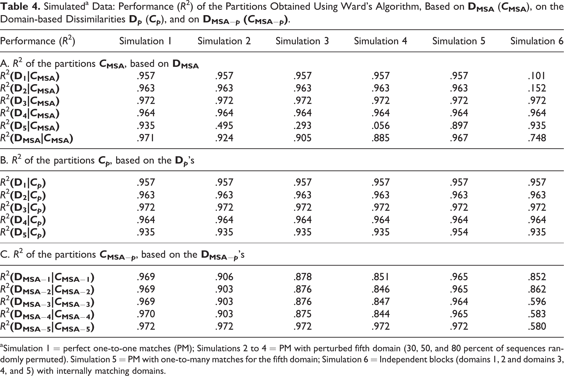
aSimulation 1 = perfect one-to-one matches (PM); Simulations 2 to 4 = PM with perturbed fifth domain (30, 50, and 80 percent of sequences randomly permuted). Simulation 5 = PM with one-to-many matches for the fifth domain; Simulation 6 = Independent blocks (domains 1, 2 and domains 3, 4, and 5) with internally matching domains.
To distinguish between domains that are possibly “difficult” to cluster and domains that are not well explained by
Note that the R
2(
We now analyze the quality of the JSA partitions obtained by removing one domain at a time. For each p, the dissimilarity matrix
Observe that in simulations 3–4 (50 and 80 percent of permuted sequences in the fifth domain), the performance notably increases when the fifth domain (not strongly related to the others) is disregarded. In this case, MSA does not provide satisfactory results for all the involved domains. Thus, the procedure is “joint,” but the quality of the results is not the same for all the domains.
These results are coherent with those obtained in the previous section. Nonetheless, this is not always the case. For simulation 5 (one-to-many matches), a low association between the fifth domain and the others was diagnosed. The analysis based on the R 2s correctly emphasizes instead that the low correlation between the fifth domain and the others does not prevent the quality of JSA (specifically MSA).
Beyond CA: Some Considerations on Other Dissimilarity-based Techniques
As already discussed, CA is only one of the techniques that can be applied using joint rather than domain-specific dissimilarities. Therefore, measures similar to those introduced earlier should also be defined for techniques which are more and more popular in SA, such as, for example, ANOVA and regression trees (Piccarreta and Billari 2007; Studer et al. 2011).
Due to space limitations, we cannot consider into detail how to extend our proposals to these methods. Nonetheless, ANOVA and regression trees are substantially based upon the evaluation of partitions defined on the basis of one or more covariates. More specifically, in ANOVA, groups are formed based on the levels of one categorical factor. The factor is significant with respect to a given domain if the factor-based groups contain similar sequences. Regression or classification trees aim instead at subsequently partitioning the sample according to the levels of one or more covariates so as to define groups of cases more and more homogeneous with respect to a given domain. Thus, in both cases, the dispersion within the (supervised) final partition’s groups plays a crucial role in the evaluation of the procedure’s results.
Evidently, for ANOVA, the dispersion within the factor-based groups can be evaluated referring both to the joint and to the domain-specific dissimilarities. Attention will be focused on the comparison of the significance of the selected factor across domains.
More interestingly, for regression trees, the final partition will be obtained by referring to the joint dissimilarities (exactly as it was done in CA; see Piccarreta and Billari [2007] for a discussion on the relations between the two techniques) and attention will be focused on the evaluation of the JSA regression tree at the domain-specific level. The procedure proposed to evaluate CA can therefore be easily extended to regression trees.
Application to the British Household Panel Survey Data
We now refer to a data set analyzed in Pollock (2007), who focuses on the first 10 years of the British Household Panel Survey. In particular, for each of the 5,124 individuals in the sample, trajectories on four domains are considered. The first domain describes the Employment (
Pollock (2007) applied MSA to the four domains, with insertion and deletion costs set to 1 and with the substitution costs matrices reported in Table 5. Based on the MSA dissimilarities, he extracted 15 clusters using Ward’s (1963) algorithm (refer to Pollock [2007] for an interesting and in-depth analysis and interpretation of the obtained clusters).
Substitution Costs Matrices.
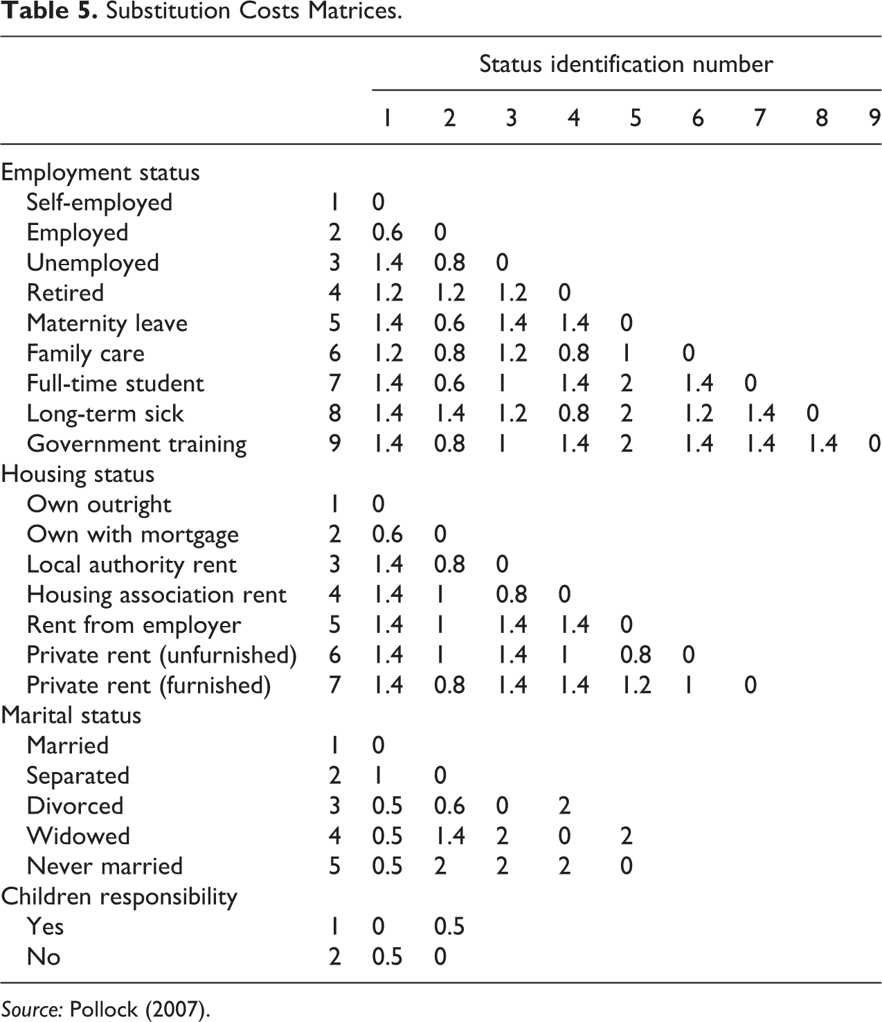
Source: Pollock (2007).
We now describe the steps of our integrated approach to evaluate the interrelations among the considered domains and the performance of a JSA both at a joint and at a domain-specific level. As already said, our evaluation is conditioned to the (chosen) domain-based and JSA dissimilarities. OM and MSA were applied using the same specifications in Pollock (2007), obtaining the dissimilarity matrices
Step 1: Preliminary Evaluation of the (Linear) Association Among the Involved Domains
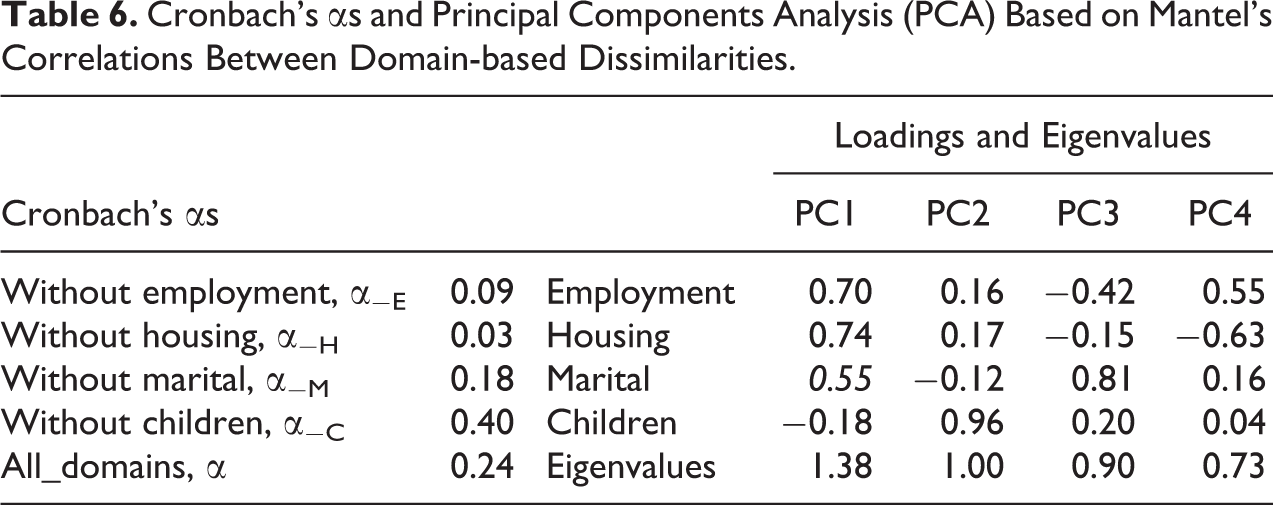
Table 6 displays the Cronbach’s αs and PCs extracted from the Mantel’s correlation matrix of the domain-based
Cronbach’s αs and Principal Components Analysis (PCA) Based on Mantel’s Correlations Between Domain-based Dissimilarities.
Step 2: Preliminary Evaluation of the (Linear) Association Between Joint and Domain-based Dissimilarities
Table 7 displays the Mantel’s correlations between the
Mantel’s Correlations Between Domain-based and MSA Dissimilarities, Sum and Mean of Squared Correlations (
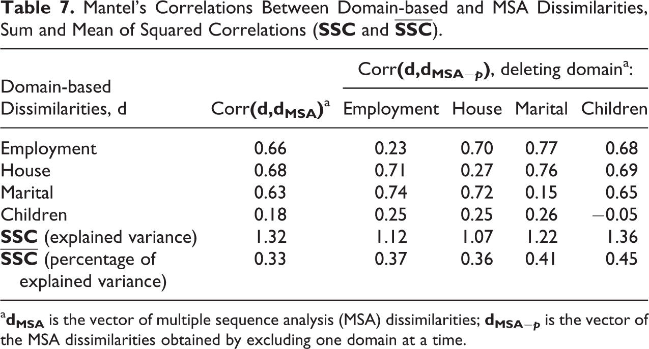
a
The weak level of detected association could make a joint analysis unable to satisfactorily “represent” each specific domain. Nonetheless, as discussed in the third section, Mantel’s correlations could fail to detect nonlinear relations. It is therefore important to directly evaluate the results obtained applying a dissimilarity-based technique on combined dissimilarities. We here focus on CA which could also conveniently describe the data, unveiling the most typical combinations of patterns across domains and shedding some light on possible nonlinear relations.
Step 3: CA Based on JSA Dissimilarities. Evaluate Partitions both at a Joint and at a Domain-specific Level
Following Pollock (2007), we applied Ward’s hierarchical algorithm to DMSA, the MSA dissimilarity matrix.
Figure 2 reports the R 2s and the average silhouette widths (Kauffman and Rousseeuw 1990) for a number of clusters ranging between 2 and 20. The silhouette coefficients suggest a rather low number of clusters (3). Moving to more detailed higher-order partitions, the six-cluster solution appears as a possible choice. Also, a steep decrease of the R 2s is observed when reducing the number of clusters from G = 6 to G = 5 (Figure 2).
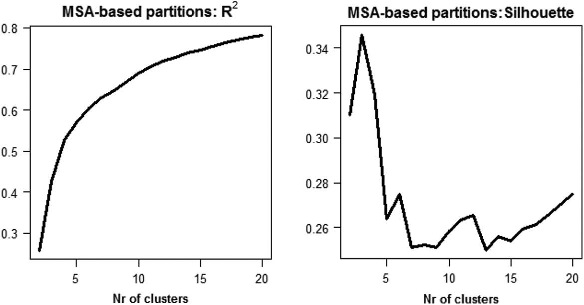
Performance (R 2 and average silhouette width coefficients) of clusters solutions obtained using Ward’s algorithm, evaluated for MSA-dissimilarities.
Since more domains are taken into account, it is important to monitor the performance of the partitions also with respect to the domain-based dissimilarity matrices (
Figure 3 displays the R 2 and the silhouette coefficients characterizing the MSA partitions evaluated with respect both to the MSA and to the domain-based dissimilarities. The number of clusters suggested by the silhouette coefficients varies with domain: Two clusters are suggested for Employment and Children, three for Housing, and four for Marital. Also, for Children, the coefficients are negative (indicating overlapping), and they become negative for all the domains when more than six clusters are taken. The plot of the R 2s shows that when G < 5 Children is left unexplained, and that when G is increased from 6 to 7, a decrease in R 2 is observed for Marital, which is again satisfactorily explained when at least nine clusters are considered.
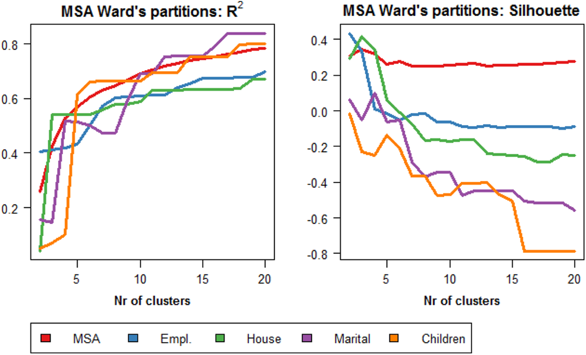
Performance (R 2 and average silhouette width coefficients) of clusters solutions obtained using Ward’s algorithm, evaluated with respect to MSA and domain-based dissimilarities.
Also, it can be noted that when G is higher than 10, the domain-specific R 2s stabilize, and a rather constant gap is observed between the R 2s for Children and Marital (aligned with the global R 2s) and those for Employment and Housing, indicating a possible division of the domains into blocks. Children and Marital turned out to be the domains least connected to the others (see steps 1 and 2). Their good explanation might therefore be due to one-to-many relations. As a further consideration, note that these domains are those with the smallest alphabets. Therefore, these domains will be easier to cluster compared to the others. A cluster procedure attempting at determining homogeneous groups of cases along all the domains might favor the simplest domains in the case of weak association (simply because the reduction of heterogeneity in the simplest domains is easier to achieve). This intuition is also supported by the analysis of the silhouette coefficients (which decrease with the number of clusters for Children and Marital, indicating overlapping).
To test these considerations in a more detailed manner and to better analyze the association among domains, we focus on a specific partition, extracting G = 6 clusters. This solution (supported by the global silhouette coefficient) is far from being optimal, and actually Pollock (2007) uses a much higher number of clusters (15). Nonetheless, we prefer a low-degree partition since its clusters can be graphically represented (see step 4 below). Also, results in Table 8 are aligned with those observed when a higher number of clusters are extracted.
Performance (R 2) of the Six-cluster Solutions (Obtained Applying Ward’s to the MSA Dissimilarities) Evaluated Both at the Joint Level and at the Domains Level.
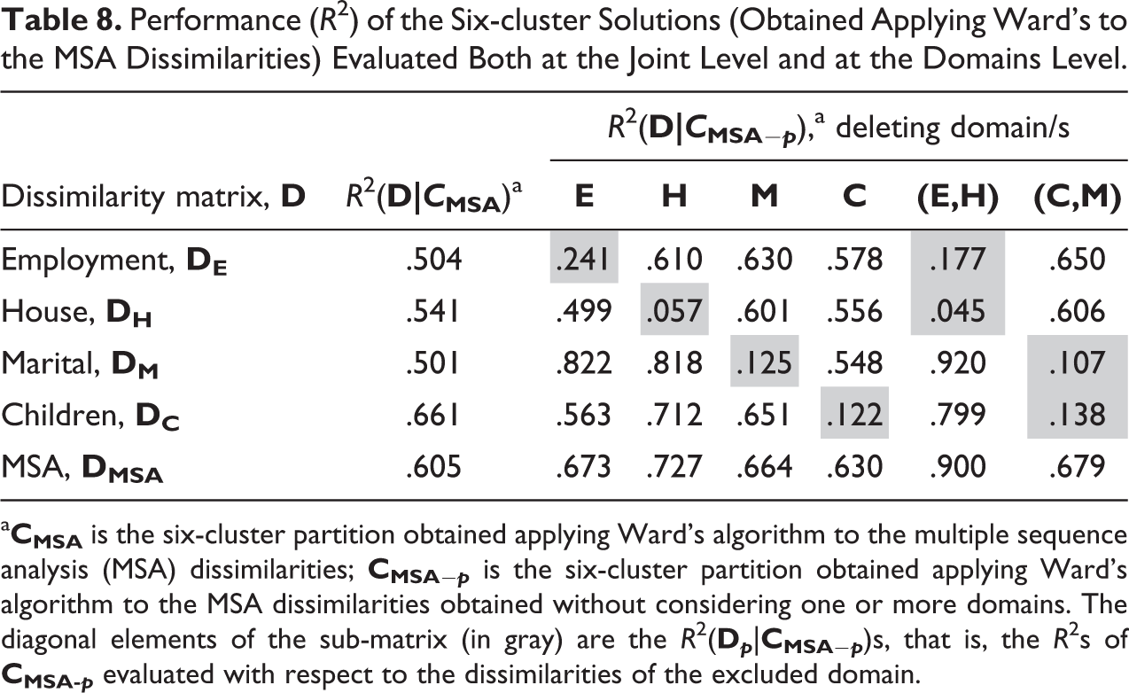
a
The first column in Table 8 shows the R
2s evaluated by referring to the MSA and to the domain-based dissimilarities. Columns 2 to 5 report the R
2s characterizing the six-cluster partitions,
The diagonal elements of the sub-matrix (cells in gray) are the R
2(
To explore also the possible division of the domains into blocks, we built the MSA dissimilarity matrices
We therefore hypothesize that (1) the four domains are split into two blocks; (2) Marital and Children, if taken into account, will always prevail over Employment and Housing, which turned out to be the most connected domains at steps 1 and 2; (3) The weak association between Children and Marital and the other domains might be due to one-to-many association. For this reason, we decided to explore the
Step 4.1: Analyzing Clusters: An In-depth Analysis Based on Graphical Tools
Our integrated approach, combining ex-ante and ex-post evaluations of the relations among domains, permits to acquire information on the opportunity and on the quality of a JSA. However, our measures are summaries: They only indicate the possible presence (or absence) of problems. When one or more domains appear to be “critical” and/or not well captured by the joint dissimilarities-based clusters, a detailed inspection of the clusters domain by domain can provide insights about the quality of the obtained clusters from a substantive point of view as well as information about the nature of the detected problems. To do so, we suggest considering index plots of the sequences in each cluster for each domain.
The plots for our data are reported in Figure 4: To each cluster, a column corresponds, with one row for each domain. In each plot, cases are placed on the horizontal axis, and to each case a vertical bar is associated describing the states experienced during the considered period of time (on the vertical axis), distinguished using different colors. The ordering of cases (in the same cluster) along the horizontal axis is the same for all the domains.
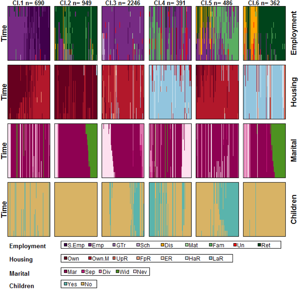
Plots of sequences grouped into the six clusters obtained by applying Ward’s algorithm to the multiple sequence analysis dissimilarities based on the Employment and the Housing domains.
These plots provide very interesting insights about the combinations of patterns in different domains as well as about the relations among the considered domains. Of course, cases in the same clusters are mostly characterized by their Employment and Housing trajectories. These trajectories are not perfectly homogeneous due to the low number of chosen clusters, but even so their (homogeneous) subclusters are clearly visible. A one-to-many association is clearly detected: Individuals with similar E–H combination are characterized by different family trajectories, as it was reasonable to expect. It is important to underline that the cluster solution based upon all the domains (not reported here) led to clusters which, being more homogeneous with respect to Children, Marital, and Housing failed to describe and capture the Employment trajectories, by far the most difficult to describe. Also, for the sake of completeness, we considered the partition obtained by referring to Employment only, and we observed a deterred cluster structure. This confirms the observed relation (steps 1 and 2) between Employment and Housing.
Interestingly, the results obtained focusing only on two domains allow us to draw conclusions even clearer than those obtained by Pollock (2007). The typologies found by Pollock using 15 clusters are clearly visible in clusters’ plots. Furthermore, the study of association permits to draw clearer conclusions on the interrelations among domains. Actually, if more clusters are considered (results not shown), groups of cases which are also homogeneous according to the excluded domains are found. Finally, it has to be pointed out that Pollock (2007) described clusters using modal combinations of states and modal switches, which did not necessarily characterize a high proportion of cases in some clusters. The description of clusters using graphical tools makes their interpretation much easier and it is surely recommended in the case when more domains are taken into account.
Step 4.2: Analyzing Clusters: Summarizing Within Clusters Dispersion
As a further piece of information, we introduce measures to identify clusters that possibly group together sequences highly heterogeneous in one or more domains. This procedure is of interest per se, but it can also be useful to understand if and to what extent a low association can be explained by costs misalignment (i.e., condition (c), the dissimilarities in the two domains increase together, is not met due to misalignments between substitution costs and closeness).
Given a partition
Evaluation of the Dispersion Within the Six-cluster Solution (Obtained Applying Ward’s to the MSA Dissimilarities Based Only on Employment and Housing) Evaluated Both at the Joint Level and at the Domains Level.
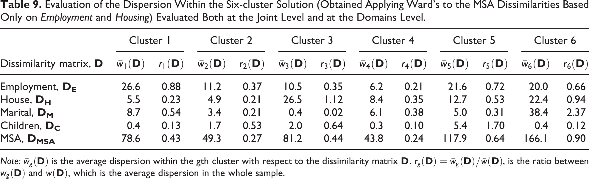
Note:
Observe in addition that the fourth cluster turns out to be the most homogeneous with respect to Employment, even if it actually includes sequences dominated by different states, namely, “Family care” and “Employed” (and to a lesser extent “Unemployed”). A low heterogeneity is detected because “Family care” and “Employed” are considered as close states based on the substitution cost matrix defined for this domain (see Table 5).
In this sense, a careful inspection and “comparison” of the plots and of the rg ’s can shed some light on the possible effects of costs definition on the domains dissimilarities and, consequently, on the joint dissimilarities and on the measures of association and dispersion.
Since the impact of the combination of the substitution costs defined on the different domains on the considered association measures is unpredictable, it could be worth to preliminarily analyze the association between domains using data-driven substitution costs (following, e.g., Rohwer and Pötter 2004, and specifying substitution costs inversely related to the frequency of transition), which do not depend on the user’s opinion (even if absolutely suitable) about the closeness or distance from one state to another.
Conclusions
The problem of jointly analyzing several domains in SA is not particularly recent. Nonetheless, many contributions propose ad hoc solutions, which are sensible and reasonable with reference to the specific considered data (Aassve et al. 2007; Blair-Loy 1999; Han and Moen 1999b; Piccarreta and Billari 2007; Stovel et al. 1996). A systematized and well-organized treatment of the problem recently appeared in Pollock (2007) and in Gauthier et al. (2010). The relevance of the problem is evident if one considers that the package TraMineR (developed for the R software; see Gabadinho et al. 2011), which is surely the most popular, now also permits to apply MSA.
Nonetheless, there are no contributions in the literature proposing methods to preliminarily evaluate the degree of interconnection between a set of domains or to evaluate the quality of the results obtained by jointly analyzing them both at a “global” and at a “specific-domain” level. With respect to the former point, some contributions exist concerning the case when two domains are taken into account. Piccarreta and Lior (2010) propose a graphical approach to visualize the relations among two domains, and Piccarreta and Elzinga (2013) introduce some criteria to quantify the strength of the association between two domains.
In this article, we innovate over the existing literature introducing an integrated approach for the ex-ante and ex-post evaluation of JSA. We start focusing on the measurement of the association between several domains and on the association between joint and domain-specific dissimilarities. Subsequently, we introduce criteria to evaluate dissimilarity-based methods applied to joint dissimilarities. There are many procedures that surely deserve attention: CA, multidimensional scaling, ANOVA, and regression trees are only some of the most used in SA.
For the sake of synthesis, we limit attention to CA. CA is surely one of the most popular techniques in SA, and it is often applied also to gain insights about the most relevant patterns in data before more structured analyses. Also, we show that the analysis of clusters can provide some further insights into the association among the domains taken into account.
We illustrate the reliability of the proposed criteria based on synthetic data, and then move to the analysis of data arising from the British Household Panel Survey, already analyzed in Pollock (2007).
Our results prove the substantive importance of our proposals. We showed how important is an exploratory analysis aiming at acquiring as much information as possible on the (possible) association among domains and its structure. The suitable identification and selection of the domains which can be efficiently studied together may prove particularly useful in SA: Looking at a too large number of domains could make the analysis unnecessarily and hopelessly overcomplex. Also, we illustrated how crucial is to assess the “joint” reliability of the results obtained using JSA and to carefully analyze the performances of the algorithms with respect to all the domains instead of focusing only on the global performance.
The assessment of association is a very useful preliminary step when more domains are studied jointly. The same of course applies when attention is focused on two domains only. As already mentioned, this topic has already been discussed in Piccarreta and Elzinga (2013). Even so, here we introduce an integrated approach which allows both testing the association and investigating the exact nature of this association. Also, our approach could be applied to compare the extent of association within subgroups (based, e.g., on gender, race, or education). Actually, finding association only in some of these subgroups, for instance, could possibly support some theoretical hypotheses or expectations about the interplay among domains (in the life course and work–family literature, for instance).
Surely, the proposed techniques can be improved along a number of directions. The definition of clear benchmarks for our measures or of permutation tests aiming at evaluating the departure from independence is clearly a relevant issue. Also, it would be surely important to define suitable criteria to evaluate JSA when applied to techniques other than CA, in particular discrepancy analysis or regression trees.
Of course, a quantitative approach as that described here is mostly useful as a screening procedure, to have some insights about solutions which merit to be inspected, and to emphasize which are the possible problems connected with the joint analysis of several domains. As for CA, for instance, the substantive interpretation of clusters plays a crucial and irreplaceable role in the choice of the partition or in the final decision about the domains to be jointly analyzed. Actually, one might be interested to extract clusters explaining all the domains in a way that is judged satisfactory, or might be prepared to obtain clusters explaining some domains worse than others. These considerations are strongly related to the goal of analysis and to the prior knowledge of the researcher on the data, which are strongly needed to support and to fully understand and interpret results.
Footnotes
Acknowledgments
All the analyses in this article were conducted using the statistical software R (R Core Team 2014). User-defined routines were used (based on a number of packages), but the dissimilarity matrices analyzed throughout this article were all obtained using the TraMineR package (![]() ).
).
The author is grateful to Gary Pollock for having shared his data and to three anonymous referees for their highly appreciable comments on a previous version of this article.
Declaration of Conflicting Interests
The author(s) declared no potential conflicts of interest with respect to the research, authorship, and/or publication of this article.
Funding
The author(s) received no financial support for the research, authorship, and/or publication of this article.