
Abstract
We consider an ordinal regression model with latent variables to investigate the effects of observable and latent explanatory variables on the ordinal responses of interest. Each latent variable is characterized by correlated observed variables through a confirmatory factor analysis model. We develop a Bayesian adaptive lasso procedure to conduct simultaneous estimation and variable selection. Nice features including empirical performance of the proposed methodology are demonstrated by simulation studies. The model is applied to a study on happiness and its potential determinants from the Inter-university Consortium for Political and Social Research.
Introduction
In the social, behavioral, and psychological sciences, ordinal data are routinely collected in surveys and can be described as a collection of ratings of individual items into ordered categories. The ordinal regression is among the most important tools to investigate the effects of explanatory variables (or predictors) on the ordinal responses of interest (see, e.g., Johnson 1996; McCullagh 1980; Moustaki 2003). Conventional ordinal regression assumes that predictors are observable and directly assessable. However, latent traits that should be characterized by several highly correlated observed indicators from different perspectives are common in many applications (Bennink, Croon, and Vermunt 2013; Bollen 1989; Lee and Song 2007; Skrondal and Rabe-Hesketh 2004). Typical examples include “life satisfaction” summarized by satisfaction in homelife, financial situation, and other things; as well as “quantitative ability” measured by test scores in mathematics, physics, and chemistry. Conventional models manage latent predictors by independently incorporating one or more of their indicators into the regression analysis. However, limitations are evident with such independent analysis. First, multicollinearity that could seriously distort the statistical inference may occur when the highly correlated indicators of a latent trait are simultaneously included in a regression. Second, given that each indicator only reflects a single characteristic of a latent trait, the independent analysis with the partial information of latent traits merely reveals incomplete relationships between variables and is therefore incapable of providing a comprehensible interpretation for the overall effect of a latent trait on the response of interest. Last but not least, high-dimensional covariates may cause the so-called curse of dimensionality problem.
The most popular technique for measuring latent variables on the basis of multiple observed indicators is the factor analysis model (Harman 1976; Kenny and Judd 1984; Lee 2007; Song and Lee 2001, among others). In this study, we propose a joint model to analyze ordinal data with latent variables. The proposed model comprises a confirmatory factor analysis (CFA) model and an ordinal regression model. The CFA model measures latent variables through correlated observed variables, whereas the ordinal regression assesses the effects of observed and latent predictors on ordinal responses of interest. Compared with conventional regression, this joint model incorporates the information from multiple indicators and thus greatly enhances its analytic power and provides scientific evidence for the effects of latent traits that are well known but hard to measure directly. The multicollinearity problem that often occurs in a regression can be naturally eliminated because the highly correlated observed variables are grouped into relatively independent latent factors through a CFA model. Under the joint modeling framework, our model simultaneously manages ordinal responses, the most important discrete data type, and unobservable predictors. Such multiple tasks cannot be accomplished by a simple regression analysis.
Although the CFA model can help reduce dimensionality of the predictors in the regression, identifying relevant predictors to obtain a parsimonious model is always of importance in statistical inference. Most contemporary research in variable selection of regression models is focused on parametric or nonparametric regression without latent variables. A majority of the existing methods lie in two directions. The first direction is the use of criterion-based procedures such as Akaike information criterion (AIC) and Bayesian information criterion (BIC) or penalized approaches in a frequentist framework, whereas the second direction is the development of Markov chain Monte Carlo (MCMC) methods including the analogues of the above procedures in a Bayesian framework. Given that the present study involves latent variables and ordinal responses, which induce an intractable likelihood function, the likelihood-based methods in the former direction are not directly applicable. On the contrary, the sampling-based Bayesian approach is feasible to provide an efficient and reliable analysis for the proposed joint model. Unlike traditional practices, which either perform a pairwise comparison via Bayesian model comparison statistics such as Bayes factor (Kass and Raftery 1995) and deviance information criterion (Spiegelhalter et al. 2002) or conduct a stochastic searching variable selection (SSVS) in the entire model space, we propose the use of a Bayesian version of the least absolute shrinkage and selection operator (lasso; see, e.g., Park and Casella 2008) to perform simultaneous estimation and variable selection in the present study. As demonstrated in the subsequent numerical studies, the Bayesian lasso (BLasso) conducts internal variable selection on model components and automatically determines an appropriate model, thereby avoiding a tedious pairwise comparison and eliminating convergence issues elicited by the varying dimensional parameter space in the implementation of the SSVS algorithm (Gilks, Richardson, and Spiegelhalter 1996).
Regularization methods such as lasso have been widely applied to substantive research in the past decades (Hoti and Sillanpää 2006; Magis, Tuerlinckx, and Boeck 2015; Tibshirani 1996). However, limitations of the lasso procedure including inconsistency in certain conditions and suffering from appreciable bias have been evident (Fan and Li 2001; Wang, Li, and Tsai 2007). To address these problems, an adaptive lasso and its variants have been proposed (see, e.g., Zou 2006). Given a high demand of Bayesian methods in the analysis of complex models and data types, the Bayesian adaptive lasso (BaLasso) has recently been developed and found to be highly efficient, conceptually simple, and easy to implement (Alhamzawi, Yu, and Benoit 2012; Leng, Tran, and Nott 2014). Nevertheless, either BLasso or BaLasso is rarely applied to the regression with latent variables. To the best of our knowledge, this is the first study to use the BaLasso procedure to conduct simultaneous estimation and model selection in the context of the proposed model.
The rest of the article is organized as follows. The second section defines the proposed model, where the ordinal responses are postulated to be associated with the underlying continuous variables. The relation between each ordinal response and its underlying continuous measurement is defined via a threshold specification. The third section develops the BaLasso procedure along with the MCMC algorithm for posterior inference. The fourth section presents simulations to demonstrate the empirical performance of the proposed methodology. The fifth section reports an application to a study of happiness and its determinants on the basis of the World Values Survey. The sixth section concludes the article with discussion. The technical details are provided in the Online Appendices.
Ordinal Regression With Latent Variables
Model Description
Let
where
Let

where β
0j
is an intercept,
Let

where
Notably, the joint model defined by models (2) and (3) is different from the conventional mixed-effect model with ordinal responses. Unlike random effects that only address the dependency of responses, the latent variables in
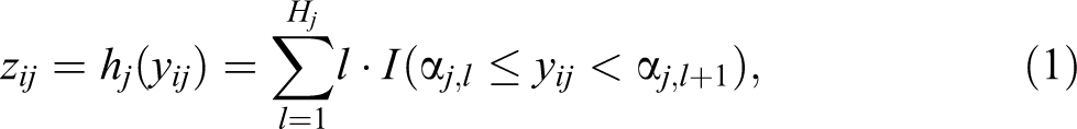
For notational simplicity, in the subsequent description, we suppress the subscript j in models (1) and (2) by assuming s = 1. Considering that yij
(and thus zij
), j = 1,…, s are conditionally independent given

where
Model Identification
The model defined in the model description subsection is not identifiable without imposing identifiability constraints. In this section, we discuss two model indeterminacies and propose appropriate identifiability constraints as follows.
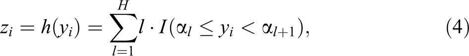
The first indeterminacy is caused by the unknown scale of the underlying continuous measurement yi
corresponding to the ordinal variable zi
, which makes the parameters
The second indeterminacy is associated with the CFA model (3). For an arbitrary nonsingular matrix
Bayesian Inference
BaLasso
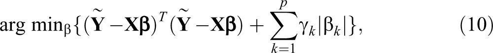
The lasso procedure that simultaneously performs parameter estimation and model selection is proposed by Tibshirani (1996) under the simple linear model framework:

where
where γ ≥ 0 is the tuning parameter, and
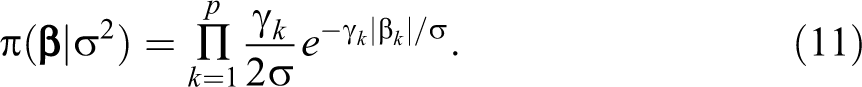
Park and Casella (2008) later introduced the Bayesian version of lasso by assigning a conditional Laplace prior of
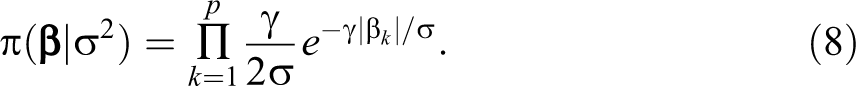
They formulated BLasso through the following hierarchical representation:
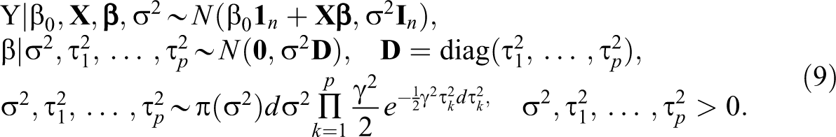
The conditional prior of
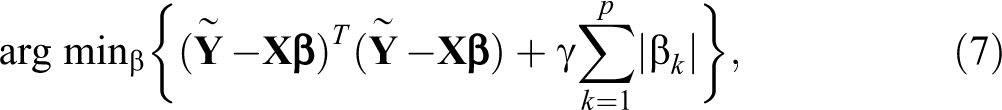
One problem with the lasso-type procedures is that the same tuning parameter γ is applied to different regression coefficients, implying that the same amount of shrinkage is introduced to all coefficients. This may add appreciable bias to the resulting estimates (Fan and Li 2001; Wang et al. 2007). To tackle the issue, Zou (2006) developed the adaptive lasso procedure, which modifies model (7) by assigning a distinct tuning parameter for each of the regression coefficients as follows:
where γ
k
≥ 0, and
Similar to the adaptive lasso, BaLasso introduces different penalties to various coefficients to enhance its capability of producing good estimation and model selection results.
As highlighted in Tibshirani (1996) and Park and Casella (2008), the lasso estimator of
Prior Specification
Based on model (10), the BaLasso estimators of the coefficients in model (5) can be defined as:
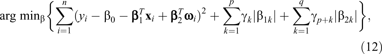
where γ
1,…,γp
+q
are nonnegative turning parameters,
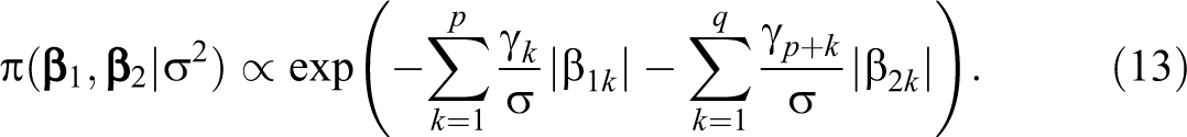
This prior distribution can be reformulated through a hierarchical model as follows (see details in the Online Appendix A):
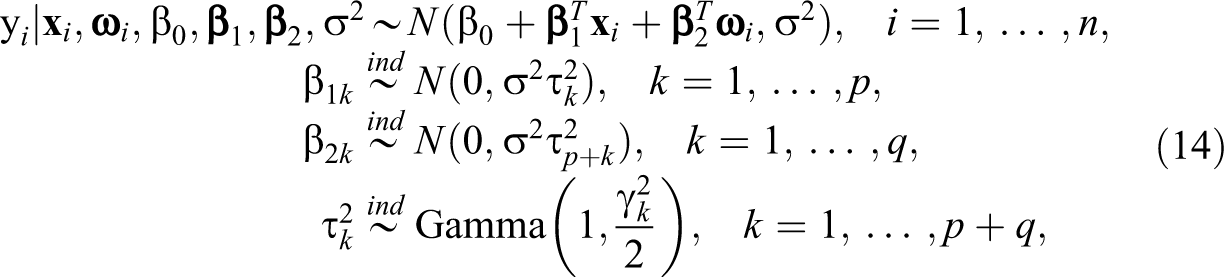
where σ 2 is fixed to identify the ordinal regression model. Given that the intercept is usually not interesting, we routinely assign a noninformative uniform prior of β 0.
For the tuning parameters γk , we assign the following gamma priors:

where ak
0 and bk
0 are hyperparameters with preassigned values. Following the suggestions of the existing literatures (e.g., Guo et al. 2012; Kyung et al. 2010; Song, Lu, and Feng 2014), we set ak
0 = 1 and bk
0 = 0.05 to obtain dispersed priors for γk
. Such dispersed priors enable γk
to be mainly determined by the data, thereby automatically imposing large penalty on unimportant coefficients and shrinking them to 0 efficiently. The reason can be found from the posterior distributions of γ
k
and

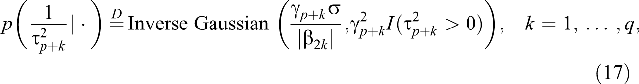

where “
For the unknown parameters in model (3), we assign conjugate type priors as follows. Let μj
and ψj
be the jth element of
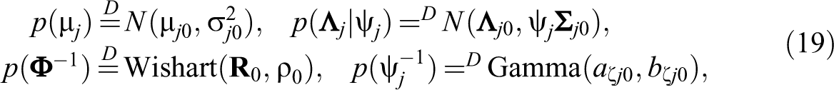
where μj
0,
Finally, we specify the prior distribution for threshold parameters. Given that thresholds are not as interesting and their information is usually unknown, we propose the use of a noninformative prior. Note that α
2 is fixed at 0 to identify the model, we let

Posterior Inference
Let
The posterior inference can be conducted by sampling from the joint posterior distribution
Simulation Study
In this section, we conduct simulations to evaluate the empirical performance of the proposed method. Simulation 1 considers a univariate ordinal regression and examines the performance of our method under different sample sizes. Simulation 2 compares the proposed method with the conventional approaches. The performance of our method in the case of s > 1 is also examined but not reported.
Simulation 1
We consider the model defined by models (3)–(5) with H = 4, p = 6, q = 4, m = 12, and three sample sizes n = 200, 500, and 1,000. The data sets are simulated as follows: covariates xi
1, xi
2, xi
3, and xi
4 are independently generated from N(0,1), ordinal (0.25, 0.25, 0.25, 0.25), U(−1, 1), and t(3), respectively, where ordinal (π
1,π
2,
π
3,
π
4) denotes a four-category ordinal distribution with probabilities (π
1,π
2,
π
3,
π
4), U(a, b) denotes the uniform distribution in [a, b], and t(3) denotes the t distribution with degrees of freedom 3. Covariates xi
5 and xi
6 are jointly generated from a multivariate normal distribution N(
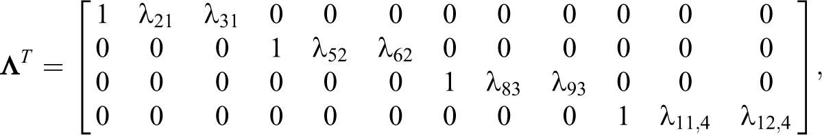
where the 1s and 0s are fixed parameters, and the λs are unknown parameters. The population values of the unknown parameters are
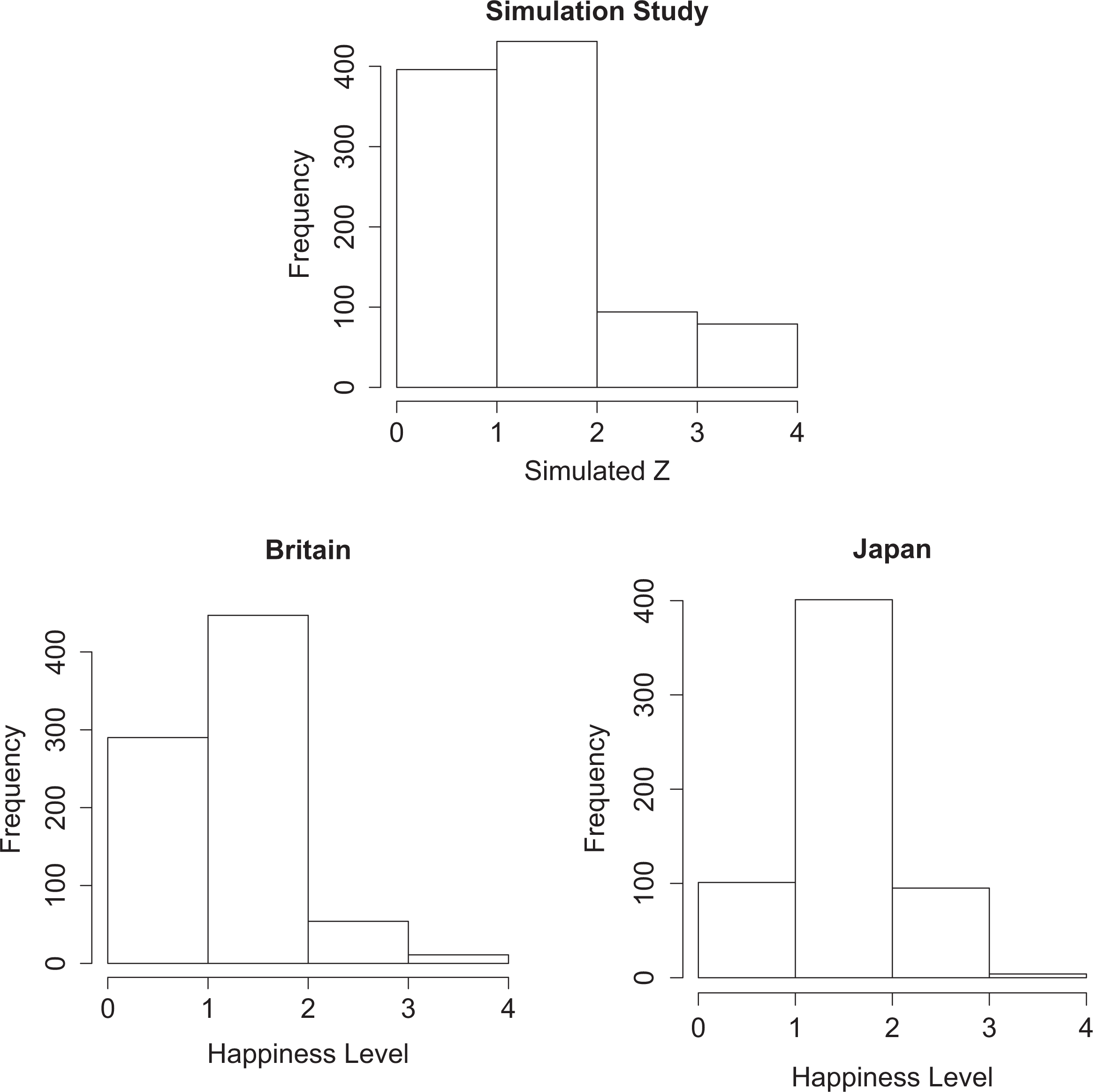
The histograms of the categorical variable z in the simulation study and the happiness data sets.
The hyperparameters of the prior distributions discussed in the subsection prior specification are specified as follows: for j = 1,…,12, μj
0 = 0, σj
0 = 100,; the elements in
The results presented below are on the basis of 100 replications. We use the bias (BIAS) and the root mean square error (RMS) of the Bayesian estimates to assess the performance of the proposed method. Tables 1 –3 report the estimation and model selection results obtained using the proposed method. The less interesting intercepts are not reported to save space. Those obtained using BLasso without adapting the turning parameter are also provided for comparison. Although both methods produce satisfactory results, the former performs better in terms of estimation and variable selection. This result is expected because BaLasso enables the data to determine the magnitude of penalty, which not only adaptively penalizes the coefficients of unimportant predictors and shrinks them to zero faster but also estimates significant coefficients more effectively. Such appealing features are demonstrated by the lower bias and RMS values under BaLasso in Table 1 and the higher correct rates produced by BaLasso in Table 3. Given that the advantage of BaLasso over BLasso is mainly focused on regression, the parameter estimates of the CFA model in Table 2 are similar for the two procedures.
Bayesian Estimates of Parameters of the Ordinal Regression Model in Simulation 1.
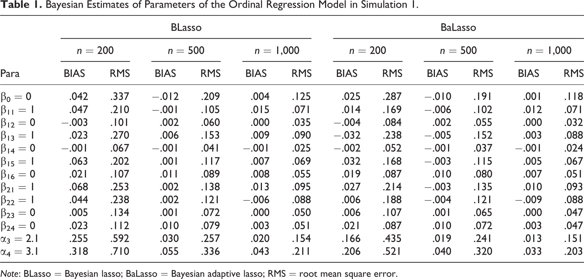
Note: BLasso = Bayesian lasso; BaLasso = Bayesian adaptive lasso; RMS = root mean square error.
Bayesian Estimates of Some Parameters of the Factor Analysis Model in Simulation 1.
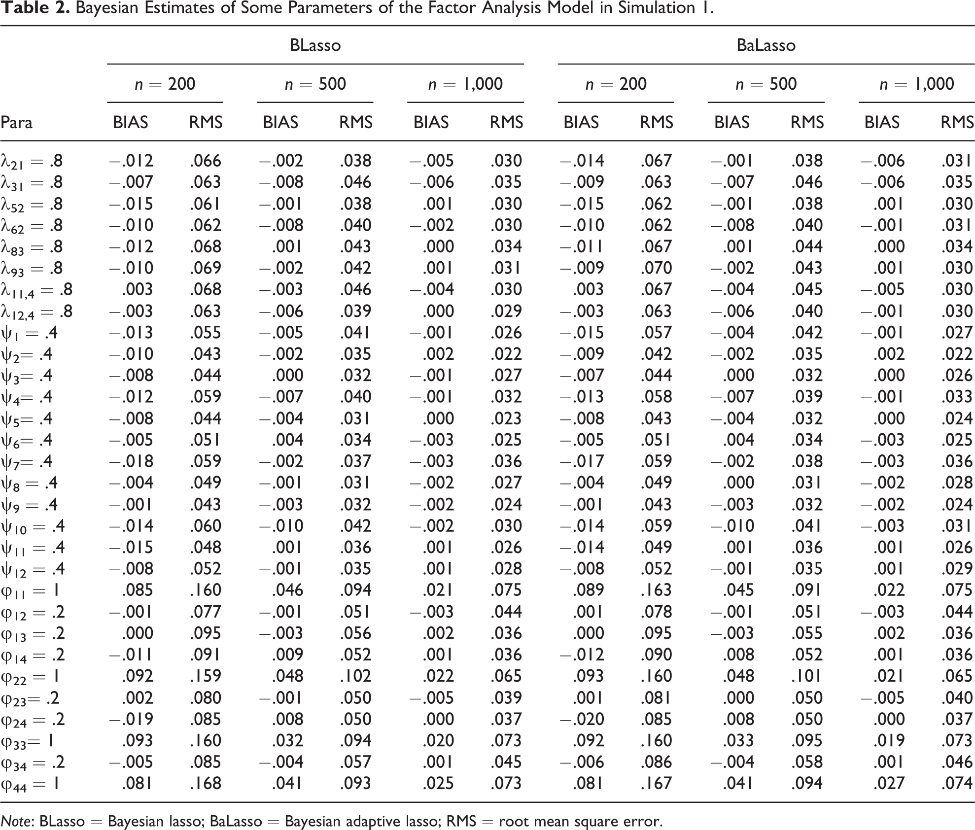
Note: BLasso = Bayesian lasso; BaLasso = Bayesian adaptive lasso; RMS = root mean square error.
Number of Correct Variable Selections in Simulation 1.
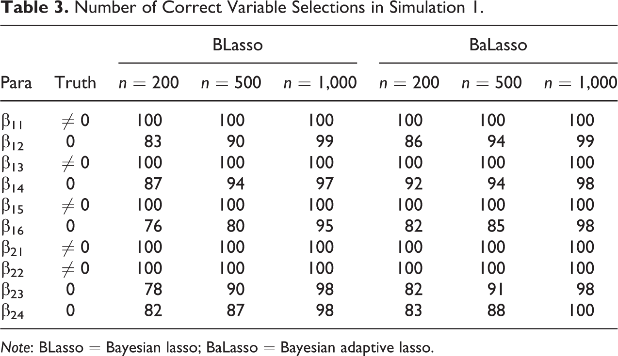
Note: BLasso = Bayesian lasso; BaLasso = Bayesian adaptive lasso.
To check whether the Bayesian results are sensitive to prior inputs, we reconduct the analysis using two different prior settings in prior (15): ak 0 = 1, bk 0 = 0.5; and ak 0 = 1, bk 0 = 0.01, together with some disturbance of other hyperparameters in prior (19). The estimation and model selection results are similar and not reported.
Simulation 2
In this section, the proposed method is compared with two conventional approaches. The first one is to simply regard the observed indicators of the latent variables as independent covariates. To compare the proposed joint analysis with such an independent analysis, the 100 replicated data sets that are generated in simulation 1 with n = 1,000 are reanalyzed using the following simple independent model:
where all the components are the same as those in simulation 1 except that here
Notably, a direct comparison in terms of estimation result is unavailable because the true value of
The second comparison is between the proposed method and a continuous regression that simply regards the ordinal response as continuous. Again, the abovementioned 100 replicated data sets with n = 1,000 are reanalyzed by treating zi as continuous. The estimates of the regression coefficients under the two methods are presented in Table 4, indicating that ignoring the ordinal nature of responses could substantially underestimate the effects of important predictors.
Comparison Between the Proposed Model and a Continuous Regression.

Note: n = 1,000. BLasso = Bayesian lasso; BaLasso = Bayesian adaptive lasso; RMS = root mean square error; N/A = not applicable.
Further, we utilize the Watanabe–Akaike information criterion (WAIC; Gelman, Hwang, and Vehtari 2014; Vehtari, Gelman, and Gabry 2015; Watanabe 2010) to compare the proposed model with the abovementioned ones that regard the observed indicators of the latent variables as independent covariates and the ordinal responses as continuous, respectively. The WAIC is defined as:

where
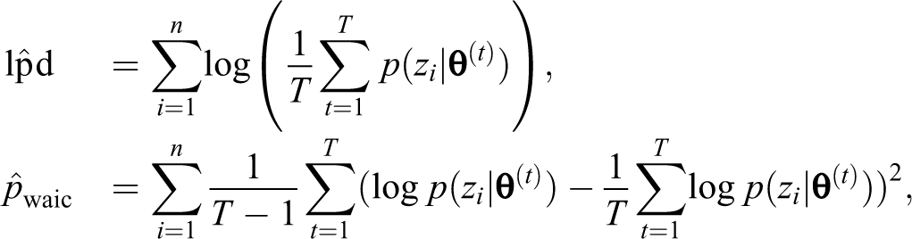
where
Figure 2 summarizes the WAIC values corresponding to the three analyses: (1) the proposed joint analysis, (2) the independent analysis, and (3) the analysis that regards ordinal variables as continuous. The box plots of WAIC values show that the proposed joint analysis substantially outperforms the others.
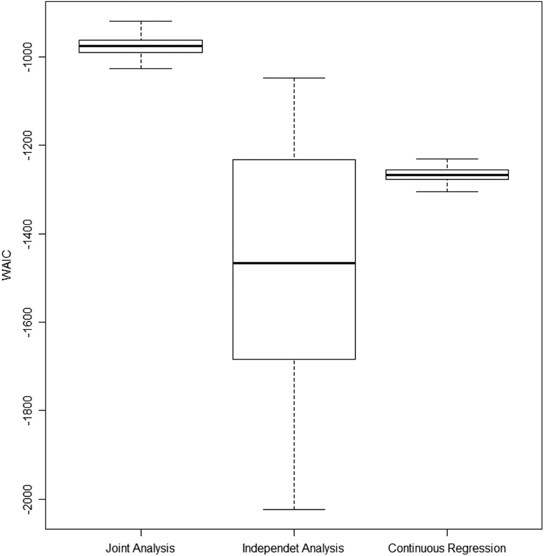
Summary of the Watanabe–Akaike information criterion values on the basis of 100 replications in simulation 2.
To examine the empirical performance of the proposed method in the case of s > 1, we likewise conduct a simulation with the exactly same set up as that of simulation 1 except s = 2. The estimation and model selection results are similar to those in simulation 1 and are not reported.
A Study of Happiness and Its Determinants
In this section, we present an application to the analysis of the World Values Survey (World Values Study Group 1994), a global research project exploring the social and personal characteristics that influence peoples’ values and beliefs. The World Values Survey collects information from participants around the world on contemporary societal issues such as individuals’ happiness, their satisfaction with life and job as well as their attitudes toward work, money, religious beliefs, and politics. The primary goal of the survey is to enable a cross-national and cross-cultural comparison of peoples’ core values. In this application, we considered the data collected from Britain and Japan, which are the typical representatives of western and eastern countries. We are particularly interested in individuals’ happiness and its major determinants, consequently discovering the culture diversity in the two populations.
A total of 802 and 601 samples were included in Britain and Japan cohorts, respectively. The ordinal response variable “happiness” (z) was measured in a 4-point scale from 1 to 4 representing very happy to not at all happy. Six observed covariates, including gender (x
1), marriage (x
2), life meaning (x
3), social–economic status (x
4), health condition (x
5), and religious belief (x
6), which are related to the characteristics of respondents, were considered as possible determinants of happiness. In addition, three latent variables such as job satisfaction (ω1), homelife satisfaction (ω2), and work attitude (ω3), which were characterized by {u
1, u
2}, {u
3, u
4, u
5}, and {u
6, u
7, u
8}, were also considered as the potential influential factors of happiness. A description of the observed indicators u
1, …, u
8, together with the abovementioned response variable z and covariates x
1, …, x
6, is provided in Online Appendix C. Given that u
1, …, u
8 were measured in a 10-point scale, we treated them as continuous. Then, the model defined by models (3)–(5) with H = 4, p = 4, q = 4, and m = 8 was proposed to conduct the analysis. A path diagram to depict the CFA model and the ordinal regression is presented in Figure 3. In the proposed model,
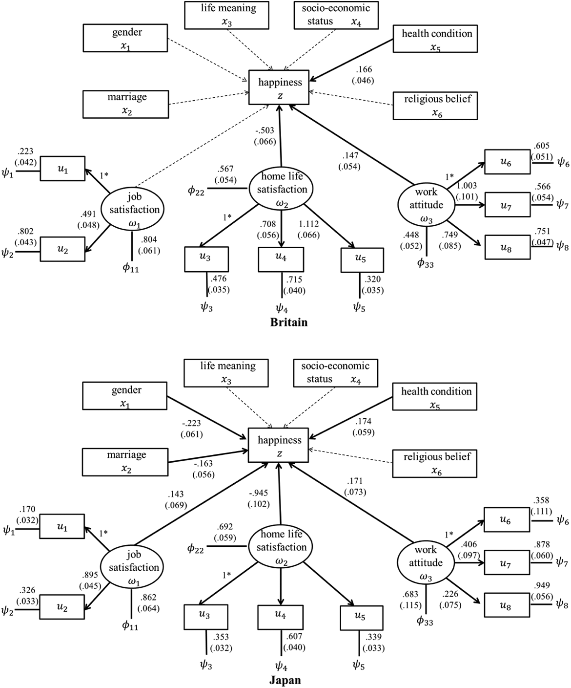
The path diagram of the proposed model, where the solid and dashed lines indicate significant and nonsignificant effects.
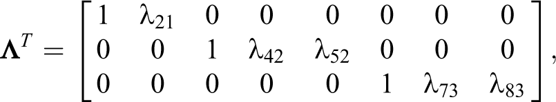
where the 1s and 0s are fixed to obtain an identified model and a clear interpretation of the latent variables.
The prior distributions discussed in the subsection prior specification with hyperparameters similar to those in simulation 1 were used. The cutoff value for identifying significant predictors was again set as 0.1. An initial estimate of the latent variables was obtained based on the CFA model for standardization. The BaLasso procedure was implemented to perform simultaneous estimation and model selection. On the basis of several testing runs starting from very different initial values, we found that the MCMC algorithm converged within 10,000 iterations. After a burn-in phase of 10,000 iterations, 10,000 additional samples were generated for Bayesian inference.
The estimated factor loadings and the significant coefficients in the ordinal regression along with their standard error estimates (in parentheses) are presented in Figure 3. For both populations, the factor loadings are substantially different from zero, indicating that each observed indicator significantly contributes to the characterization of the associated latent variable. Based on their operationalization, the latent variables can be interpreted as follows. Higher scores of ω
1 and ω
2 imply better satisfaction with job and homelife. An increase in the score of ω
3 indicates a more negative attitude toward job. For the British, the significant predictors include health condition (x
5), homelife satisfaction (ω
2), and work attitude (ω
3). Their estimated coefficients are In both countries, health condition (x
5) and homelife satisfaction (ω
2) are closely related to happiness. Healthier people and those with higher satisfaction with their homelife tend to be happier. This result agrees with previous studies (see, e.g., Lee and Ono 2008; Stack and Eshleman 1998), in which similar associations were discovered. Another common determinant of happiness shared by the two cohorts is work attitude (ω
3). Active work attitude in general raises happiness. Mohanty (2009) also revealed the tie between happiness and positive attitude toward life, work, and daily affairs. The effects of gender (x
1) and marriage (x
2) on happiness are nonsignificant for the British but significant for the Japanese. In general, female and married Japanese are happier than male and unmarried ones, respectively. This conclusion aligns with the previous findings (Lee and Ono 2008; Oshio and Kobayashi 2010, 2011; Stack and Eshleman 1998), which investigated the gendered division of labor, marriage, family roles as well as their impacts on happiness, in Japan. In Britain cohort, the effect of job satisfaction (ω
1) on happiness is again nonsignificant, implying that the British have better work–life balance and seem less dominated by job. However, this effect is negative in Japan cohort. A possible reason is that high job satisfaction may make the Japanese greatly devote themselves to job, consequently reducing their homelife quality and lowering their happiness. This finding has a good agreement with those of Greenhaus and Beutell (1985) and Shimazu et al. (2011). For both populations, life meaning (x
3), socioeconomic status (x
4), and religious belief (x
6) are all irrelevant to happiness. Whether or not this conclusion can be generalized to other western or eastern countries requires further investigation.
For comparison, we conducted an independent analysis by incorporating u
1, …, u
8 as independent covariates into the regression. The estimated coefficients of x
1, …, x
6 are similar and not reported. Those corresponding to the latent variables are reported in Table 4, which shows that all the u
1, …, u
8 become nonsignificant. Specifically, the estimates of
Comparison of the Joint and the Indepedent Analyses of Happiness and Its Determinants.

Note: WAIC = Watanabe–Akaike information criterion.
To assess the sensitivity of the Bayesian inference to the prior inputs, the analysis was repeated by disturbing the prior inputs in a similar manner as that in simulation 1. The estimation and model selection results are close to those reported in Figure 3.
Discussion
In this article, we considered a simultaneous estimation and model selection for the ordinal regression with latent variables. Ordinal responses were formulated via the underlying continuous measurements with a threshold specification. A BaLasso procedure coped with MCMC methods was developed to conduct the analysis. The empirical performance of the proposed methodology was demonstrated by simulations. An application to a study of happiness and its determinants in Britain and Japan was presented.
The current study has limitations. First, we only considered the linear effects of predictors on ordinal responses. This linear assumption may not be true in practice. Extending the proposed parametric model to a nonparametric framework is of scientific interest. Bayesian nonparametric techniques such as Bayesian penalized splines (Lang and Brezger 2004) and Gaussian process (Rasmussen and Williams 2006) are plausible techniques for this generalization. Second, although ordinal data are of the most common data type, a comprehensive model accommodating a wide variety of data types shows high potential in real applications (Song et al. 2013; Wang, Feng, and Song 2015). Finally, we characterized latent variables on the basis of multiple observed indicators via a CFA model, in which the number of latent factors and the operationalization of latent constructs are given in advance. While substantive study and common knowledge often provide such kind of information, an exploratory factor analysis that determines the number of latent variables and their observed indicators fully by data is highly useful in practice. A generalizable approach for simultaneously operating latent factors and selecting relevant predictors is a promising attempt but requires further investigation.
Footnotes
Declaration of Conflicting Interests
The author(s) declared no potential conflicts of interest with respect to the research, authorship, and/or publication of this article.
Funding
The author(s) disclosed receipt of the following financial support for the research, authorship, and/or publication of this article: This research was supported by GRF 14305014 from the Research Grant Council of the Hong Kong Special Administration Region, NSFC 11471277 from the National Natural Science Foundation of China, and CUHK 4053138 from the Direct Grant of the Chinese University of Hong Kong.
Supplemental Material
Supplementary material for this article is available online.
References
Supplementary Material
Please find the following supplemental material available below.
For Open Access articles published under a Creative Commons License, all supplemental material carries the same license as the article it is associated with.
For non-Open Access articles published, all supplemental material carries a non-exclusive license, and permission requests for re-use of supplemental material or any part of supplemental material shall be sent directly to the copyright owner as specified in the copyright notice associated with the article.