
Abstract
Areal data have been used to good effect in a wide range of sociological research. One of the most persistent problems associated with this type of data, however, is the need to combine data sets with incongruous boundaries. To help address this problem, we introduce a new method for identifying common geographies. We show that identifying common geographies is equivalent to identifying components within a k-uniform k-partite hypergraph. This approach can be easily implemented using a geographic information system in conjunction with a simple search algorithm.
Introduction
As recent reviews suggest, there is a growing interest in the way in which social processes are influenced by the effects of place and space (see Gieryn 2000; Lobao, Hooks, and Tickamyer 2007; Logan 2012). Much of the work in this tradition draws on spatially referenced data compiled at the level of areal units such as census tracts, metropolitan statistical areas, counties, and so on. Unfortunately, the utility of areal data is often compromised by changes in the boundaries of the units in question. Such changes are akin to changes in the composition of the underlying sample and thus undermine our ability to compare units over time. Similar problems can arise when attempting to merge cross-sectional data combining different units of analysis.
While there are conditions under which the effects of boundary changes can be modeled directly (see Gutmann, Deane, and Witkowski 2011), this issue is more commonly addressed through procedures such as aggregation (Horan, Hargis, and Killian 1989) and areal interpolation (Downey 2006; Markoff and Shapiro 1973; Reibel 2007; Saporito et al. 2007), both of which capitalize on the ability to harmonize geographic data. Toward this end, we introduce a new method for identifying commonalities between sets of geographically incongruous observations. To anticipate our main finding, we show that identifying common geographies is, by definition, equivalent to identifying the components of a k-uniform k-partite hypergraph. This approach can be easily implemented using a geographic information system (GIS) in conjunction with a simple search algorithm.
Identifying Common Geographies
Areal units are created by dividing a continuous space into a set of discrete territories commonly referred to as zones. Here, we use the term partition to refer to the resulting set of zones. Geographic incongruity—the problem we are trying to address—results from the fact that the same space can be partitioned in multiple ways. The relationship between partitions is represented by their intersection, as illustrated in Figure 1, which depicts the intersection between a pair of hypothetical partitions A and B. We use the notation A × B to denote the intersection between A and B. A pair of zones is said to intersect if they share common territory. If we look closely at A and B, we see that the two partitions share a number of common boundaries. As highlighted in the rightmost panel of Figure 1, these boundaries make up a new set of geographies that are common to both A and B.
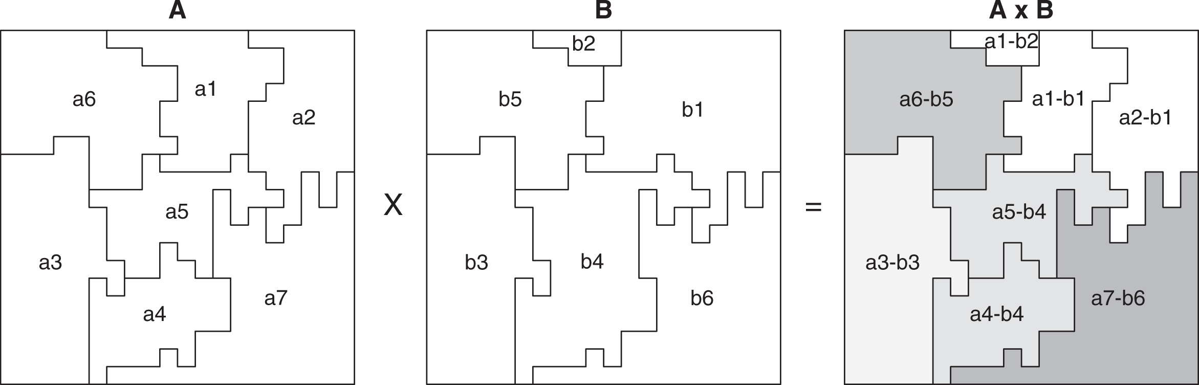
Example of intersections and common geographies. Note: Shading indicates a common geography.
For any given set of k partitions, there exists a corresponding set of one or more common geographies. Common geographies can be derived from the relationships resulting from the intersection of the original partitions. The relationships associated with the intersection of A and B are recorded in the first two columns of Table 1 which together make up what is known as an edge list, a standard tool for representing network data (see Newman 2010:111, 298-301). Each row of the table represents a unique edge, as indicated by the assignment of edge IDs. Formally speaking, edges are said to be made up of subsets of vertices. In this particular case, vertices refer to zones. Zones belonging to the same edge are tied to one another by virtue of sharing a common territory. This can be seen by comparing Table 1 to Figure 1. Each edge refers to both an observed relationship and a discrete territory. Going down the table row by row, we can confirm that there are regions in the hypothetical space corresponding to the intersection of zones a1 and b1, zones a1 and b2, zones a2 and b1, and so on. By the time we reach the end of the table, we will have covered the entire space in question.
Intersections, Edges, and Components for Partitions A and B.
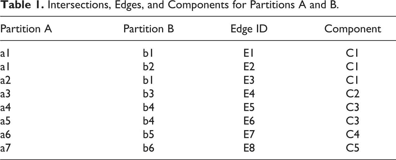
The set of edges forms a k-uniform k-partite hypergraph, meaning that not only is each edge composed of exactly k vertices, but the the set of vertices can also be divided into k classes—one for each partition. In the example at hand, k = 2, thus giving us the 2-uniform 2-partite hypergraph shown in Figure 2. Each edge is represented by a circle enclosing the subset of vertices to which the edge refers. In each case, we find two vertices, the first of which is associated with a zone from A and the second of which is associated with a zone from B. We also find that every vertex belongs to at least one edge, with a number of vertices belonging to more than one, as indicated by the presence of overlapping circles. From this perspective, each vertex can be thought of as a subset of edges, in much the same that each edge can be thought of as a subset of vertices. The difference is that whereas an edge refers to zones sharing a particular territory, a vertex refers to the territories combined in a single zone.

2-uniform 2-partite hypergraph.
The resulting graph is made up of five components, each of which corresponds to a common geography. In effect, each component contains k manifestations of a single region. This can be most easily seen in the case of components C2, C4, and C5, each of which is comprised of one edge containing two geographically equivalent zones. The common geography associated with component C2, for example, can be variously represented using either zone a3 or zone b3. Without looking at the map, we know these zones are geographically equivalent by virtue of the fact that they belong to the same set of edges (E4) and thus combine the same territories. This same principle applies to groups of zones as well. Consider the case of component C1, which is made up of four vertices (a1, a2, b1, b2) distributed across three edges (E1, E2, E3). Zones a1 and a2 collectively belong to edges E1, E2, and E3, as do zones b1 and b2. So while none of the zones in C1 are geographically equivalent, zones a1 and a2 are collectively equivalent to zones b1 and b2. As such, the common geography associated with component C1 can be variously represented using either zones a1 and a2 or zones b1 and b2. If we repeat this exercise for component C3, we find that zones a4 and a5 are collectively equivalent to zone b4.
The above example is simple and completely generalizable. A component refers to a maximal connected subgraph—a subset of vertices that are directly or indirectly connected to one another but disconnected from all other vertices in the graph. The key point for our purpose is that components contain both a subset of vertices and the subset of edges to which the vertices in question belong. This is the basis for collective geographic equivalence. As such, the components of the k-uniform k-partite hypergraph depicting the relationships associated with the intersection of any given set of k partitions must refer to a set of common geographies, regardless of the number of partitions being considered, the resulting number of components, or the density of ties within any given component. Moreover, the set of components refers to the largest possible set of common geographies that can be recreated from the original data. So while one could reasonably imagine trying to identify smaller geographies by allowing components to be divided into blocks, cliques, or communities, the vertices that make up the resulting entities will not necessarily refer to the same territory.
Implementation
In the previous section, we showed that for any given set of k partitions, there exists a corresponding set of common geographies. More specifically, we showed that, by definition, identifying common geographies among a set of k partitions is equivalent to identifying the components of a k-uniform k-partite hypergraph. How does this work in practice? We proceed in three steps. First, we use a GIS to calculate the intersection of the partitions in question. Second, we use the resulting information to construct an affiliation matrix depicting the relationship between vertices and edges in the corresponding hypergraph. Third, we assign edges to components using a simple search algorithm.
Calculating the Intersection of Partitions
We use the GIS to construct a new partition representing the intersection of the set of k partitions from which we begin. GIS packages differ in terms of the number of geographies that can be intersected at any one time. In cases where the full set of intersections cannot be calculated directly, we proceed iteratively (i.e., we calculate A × B by calculating the intersection between A and B, A × B × C by calculating the intersection between A × B and C, etc.). When asked to calculate an intersection, most GIS routines will naturally return an edge list. As per the example in Table 1, we assign a unique identifier to each edge. So long as each edge is uniquely identified, the choice of ID is arbitrary. At this stage, vertices should at least be uniquely identified within partitions. This rule is typically enforced by the GIS.
Constructing an Affiliation Matrix
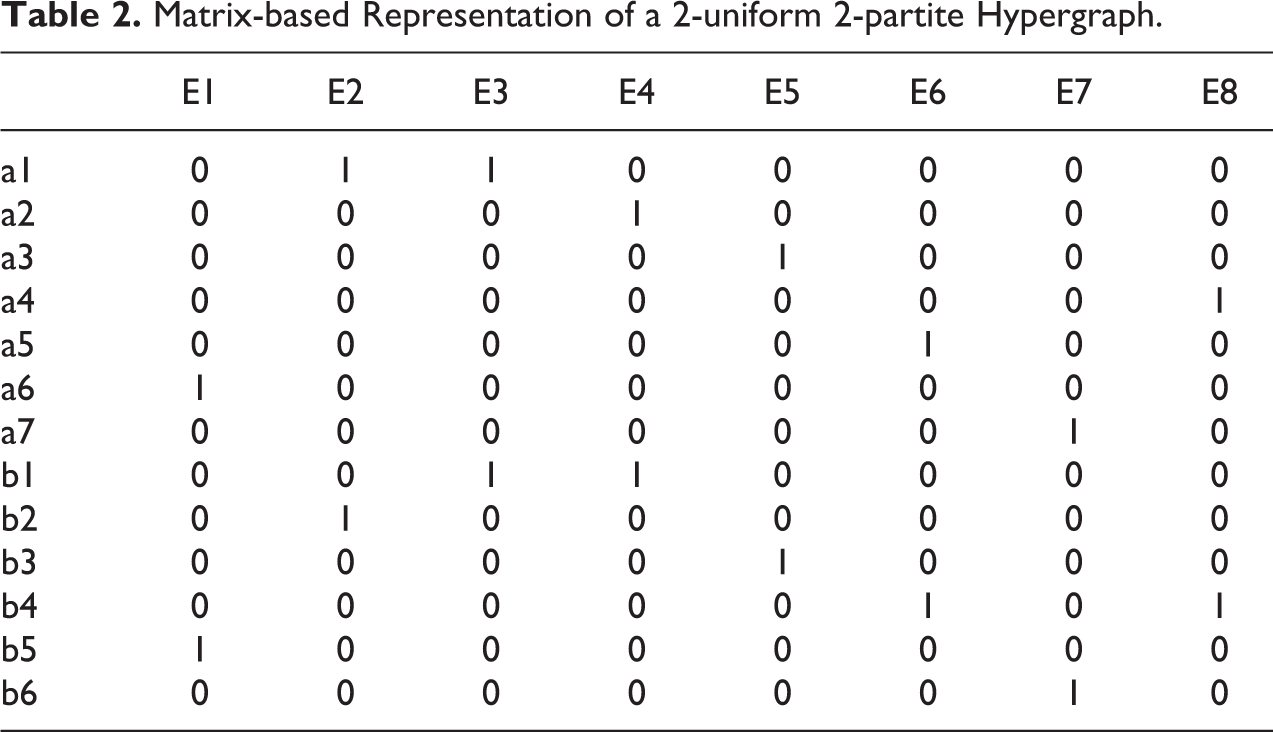
The next step is to convert the edge list contained in Table 1 into an affiliation matrix such as the one in Table 2. We begin by reshaping Table 1, such that each of the observed vertex–edge combinations appears as a separate row (i.e., we convert the data from “wide” to “long”). In the process, the first k columns of the original edge list are replaced with a pair of variables indicating (a) the name of each vertex and (b) the partition from which it was drawn. If vertices are not uniquely identified across partitions already, a unique identifier can be constructed from the name and partition variables. Next, we construct a series of dummy variables indicating whether the observation in a given row belongs to a given edge. Finally, we collapse the data by taking the within-vertex sum of each of the dummy variables.
Matrix-based Representation of a 2-uniform 2-partite Hypergraph.
Identifying Components
Having constructed an affiliation matrix, the final step is to assign edges to components, as per the example in Table 1. Affiliation matrices are often transformed prior to analysis, with transformations typically taking one of two forms. Given an n × m affiliation matrix
For the purposes of identifying components, the choice of transformation (i.e., block diagonal, vertex-to-vertex, or edge-to-edge) is irrelevant, in that, by definition, edges must belong to the same component as the vertices of which they are comprised and vice versa. The decision to focus exclusively on edges is largely a matter of convenience related to the structure of the edge list from which we began. The chief advantage of building around this particular data structure is that it naturally separates groups by partition while retaining the original identifiers used in the geographic data. The components of the graph associated with
Discussion
The procedure described above is most directly applicable to the construction of aggregated geographies. Table 1 is, in effect, an aggregation schedule, in that it tells us which elements of a given partition need to be aggregated in order to recreate the underlying set of common geographies. The tabular data associated with each of the partitions are aggregated to match the newly defined geographies. Until now, the identification of common geographies has been arduous enough to require the use of predefined aggregation schedules, perhaps the most popular of which is the County Longitudinal Template (CLT; Horan and Hargis 1995). As described by Horan et al. (1989:110), the CLT is organized around a “‘current counties-to-past counties’ transformation matrix” consisting of a series of decennial “transformation vectors” used to assign counties in the contemporary United States to a set of geographically stable clusters, thus allowing for interdecennial comparison across several decades.
Not surprisingly, the CLT produces suboptimal results when applied to questions for which it was not designed (see Tolnay, Deane, and Beck 1996:799 footnote 12). In general, it is difficult to anticipate the exact demands of any given research project, thus making it unlikely that the necessary template will be available when needed, if only because existing templates are perpetually going out of date, as clearly evidenced by the case of the CLT which was last updated in 1990. Our method can be used in the same spirit as the CLT, the difference is that our method creates aggregation schedules on the fly, thus allowing them to be tailored to any project. 1 Our approach can also be used to facilitate the use of areal interpolation, a procedure typically described in opposition to aggregation (see Downey 2006:580-82; Gregory and Ell 2005:151-53). Whereas the goal of aggregation is to engineer comparability by combining otherwise incongruous units, the goal of areal interpolation is to project values from a set of “source” units onto a set of “target” units, with the latter serving as a stable point of geographic reference.
The basic idea behind areal interpolation is that each source contributes values to the targets with which it intersects, such that yt = ∑ syst , where yt refers to the estimated value associated with a given target t and yst refers to the contribution “sent” from s to t. Insofar as yst is unobserved, areal interpolation is, in effect, a solution to a missing data problem (Flowerdew and Green 1994). The resulting data are estimates and thus introduce the threat of measurement error, the effects of which are well known (see Davidson and MacKinnon 2004:312-14). Whether measurement error is a problem depends on the accuracy of the estimates. With this issue in mind, we argue that common geographies can be productively integrated into the interpolation process, as evidenced, for example, by the work of O’Connell (2012), who models the relationship between slavery and racial inequality in the present-day American South by linking data from the 2000 census to historical census data dating back to 1860. To do this, O’Connell uses information on the distribution of the county-level population in 2000 to project aggregated data from 1860 on to the 2000 boundaries.
The advantage of this approach is that it provides a simple method of preserving observations while using population data to inform the estimation process, a procedure which has been shown to improve the accuracy of interpolation (see Saporito et al. 2007). Deriving accurate estimates is the first step in producing usable data. Yet the question of how to correctly model areally interpolated data remains an open area of inquiry. There are good reasons to think that common geographies have a role to play here, too. Insofar as each source contributes to the set of targets with which it intersects, areal interpolation is structured around the same set of relationships used to identify common geographies. In effect, common geographies serve to demarcate the regions within which interpolation occurs. To put it another way, any given set of areally interpolated data has a corresponding set of common geographies lurking below the surface.
This has important implications for how we approach the modeling process. While some common geographies refer to a single geographically stable target, others refer to clusters of interdependent targets bound together by virtue of sharing common sources. In addition to being interdependent, clustered observations may differ from their stable counterparts in other ways as well. At the very least, we know that interpolation-induced errors only accumulate within clusters, thus pointing to the possibility of groupwise heteroskedasticity, with each common geography serving as a latent group. In the face of such possibilities, we can use information on the composition of common geographies to help build a better model. The utility of common geographies thus extends well beyond aggregation. Fortunately, the identification of common geographies is no longer the task it once was. As we have shown, common geographies can be easily identified using standard methodological tools, thus providing a tool which is both flexible and readily deployed.
Footnotes
Authors’ note
The Online Appendix includes sample code for both Stata and R. The analyses above can also be carried out using aiR, a standalone R package available through the first author’s website. The package can be installed directly in R using the install_github function included as part of the devtools package (![]() ). Once devtools is installed, aiR can be installed using the following command: devtools::install_github(“aslez/aiR”).
). Once devtools is installed, aiR can be installed using the following command: devtools::install_github(“aslez/aiR”).
Acknowledgment
The authors wish to thank Jeff Blossom, Russell Dimond, Alex Hanna, John Levi Martin, and Matt Salganik for their helpful comments and suggestions.
Declaration of Conflicting Interests
The author(s) declared no potential conflicts of interest with respect to the research, authorship, and/or publication of this article.
Funding
The author(s) received no financial support for the research, authorship, and/or publication of this article.
Note
References
Supplementary Material
Please find the following supplemental material available below.
For Open Access articles published under a Creative Commons License, all supplemental material carries the same license as the article it is associated with.
For non-Open Access articles published, all supplemental material carries a non-exclusive license, and permission requests for re-use of supplemental material or any part of supplemental material shall be sent directly to the copyright owner as specified in the copyright notice associated with the article.