Model-Based and Design-Based Inference: Reducing Bias Due to Differential Recruitment in Respondent-Driven Sampling

Abstract

Respondent-driven sampling (RDS), a link-tracing sampling and inference method for studying hard-to-reach populations, has been shown to produce asymptotically unbiased population estimates when its assumptions are satisfied. However, some of the assumptions are prohibitively difficult to reach in the field, and the violation of a crucial assumption can produce biased estimates. We compare two different inference approaches: design-based inference, which relies on the known probability of selection in sampling, and model-based inference, which is based on models of human recruitment behavior and the social context within which sampling is conducted. The advantage of the latter approach is that when the violation of an assumption has been shown to produce biased population estimates, the model can be adjusted to more accurately reflect actual recruitment behavior, and thereby control for the source of bias. To illustrate this process, we focus on three sources of bias, differential effectiveness of recruitment, a form of nonresponse bias, and bias resulting from status differentials that produce asymmetries in recruitment behavior. We first present diagnostics for identifying types of bias and then present new forms of a model-based RDS estimator that controls for each type of bias. In this way, we show the unique advantages of a model-based estimator.

Keywords

respondent-driven sampling network sampling hidden populations Markov RDS

Introduction

Respondent-driven sampling (RDS; Heckathorn 1997, 2002, 2007; Salganik and Heckathorn 2004; Volz and Heckathorn 2008) is a link-tracing sampling method that is able to reach hidden populations, such as sex workers (Johnston et al. 2006), men who have sex with men (MSMs; Deiss et al. 2008; Johnston et al. 2008; Millett et al. 2007; Ramirez-Valles et al. 2005), injection drug users (IDUs; Abdul-Quader et al. 2006; Frost et al. 2006; Stormer et al. 2006; Wang et al. 2005, 2007), and undocumented immigrants (Bernhardt et al. 2009; Montealegre et al. 2013). It is both a form of network sampling and a framework of statistical inference. As a sampling procedure, RDS begins with a convenience sample of initial subjects who serve as “seeds” and then through social connections seeds recruit peers who compose the sample’s “first wave.” The first wave then recruits the second wave, and the sample expands in this recursive manner, wave by wave, until the desired sample size has been reached. Finally, after completing per recruitment, respondents return to the interview site to receive rewards for having recruited peers. This provides the opportunity for a “postinterview” focusing on factors such as who they tried to recruit and who refused. The advantage of RDS is that it provides a means for drawing probability samples of populations which cannot be effectively sampled using traditional population survey methods because they lack a sampling frame and because population members have social networks that are hard for outsiders to penetrate due to stigma or privacy concerns.

As a statistical framework of inference, two major approaches have been developed. The first approach employs a model based on the recognition that recruitment in RDS involves respondents recruiting their acquaintances, friends, and those closer than friends, all of which are examples of reciprocal ties. An implication is that ties between any two groups are equal in both directions, for example, those whom I consider to be my acquaintances also generally consider me to be one of their acquaintances. Therefore, the model is termed the “reciprocity model” (Heckathorn 2002, 2007; Salganik and Heckathorn 2004). The estimations build on this basic feature of social structure that underpins the hidden population. Because estimation is based on assumptions about the structure of the network linking the target population, this is an example of a model-based approach. The model-based RDS estimators we consider in this article are SH2004 (Salganik and Heckathorn 2004) and H2007 (Heckathorn 2007). We do not consider a further model-based RDS estimator developed by Gile and Handcock (2015) because its model is not sufficiently specified to permit simulation analysis.

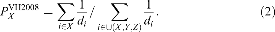
The second approach to estimation from RDS data sets relies only on the estimated probability of selection derived from the sampling design. Specifically, the probability of selection is assumed to be proportional to respondents’ degrees, that is, their number of friends and acquaintances. This fits estimators such as VH2008 (Volz and Heckathorn 2008). Since this type of estimation is dependent on the designed sampling procedure with no reference to the assumptions of underlying social networks or human behavior, it is an example of a design-based approach. Although much work has been devoted to comparing the performance of these model- and design-based approaches under various assumptions and conditions (e.g., see Gile and Handcock 2010), the source of the difference of performance between them is not well understood because the comparisons were based on simulations rather than analytic approaches. Therefore, it is unclear what level of consistency will be found if the conditions of the simulations are altered. It is the goal of the article to clarify the difference between these two approaches and demonstrate the advantage of the model-based approach in combining probability samples and sociological understanding of the hidden population.

In this article, we focus on what we term differential recruitment bias (DRB), an important bias in RDS estimation arising from different recruitment tendencies among groups. An example is provided in a study of Latino MSM in Chicago (Ramirez-Valles et al. 2005). This bias is produced by two interrelated factors. First, HIV-positive Latino MSM recruited more peers, on average, than did those who are HIV negative. This is termed differential recruitment effectiveness (DRE), and it can result from a combination of factors, such as the group giving out more recruitment coupons, their coupons being accepted by the intended recipient in greater numbers, or more of the coupons being used by the recipient to enter the study. Second, HIV-positive Latino MSM had differing recruitment patterns (DRPs) than did negatives. This consisted of respondents tending to recruit peers from their in-group, specifically, positives recruiting positives, a pattern known as “homophily.” In combination, differential recruitment effectiveness and recruitment patterns produce DRB. In this case, the bias consists of oversampling of HIV positives, because positives did more recruiting (i.e., DRE) and tended to recruit one another (i.e., DRP), resulting in a greater proportion of positives in the sample (i.e., 0.247) than in the population (i.e., 0.168) from which the sample was drawn (DRB). A similar example concerns female jazz musicians in New York City (Heckathorn 2007). Females were more effective recruiters and they recruited other females in disproportionate numbers, so the combined effect of these factors was oversampling of females, so the proportion of females in the sample (i.e., 0.263) was greater than the proportion of females in the population of New York (NY) jazz musicians (i.e., 0.238). Hence, again, a combination of DRE and DRP produced DRB.

Differences between our terminology and that which is employed in other papers should be noted. For example, in Tomas and Gile (2011), differential recruitment is defined as preferential selective recruitment, in which respondents pass coupons at a distinct rate to contacts who have certain group characteristics. This bias should be characterized as differing recruitment pattern, which alone cannot generate bias in the population estimate. It has been demonstrated in their paper that the difference between SH2004 and VH2008 is negligible in the presence of preferential selection of recruitment. We find it important to differentiate among the three terms, DRE, DRP, and DRB, because each plays quite different roles in RDS estimation. For example, in isolation, the first, DRE, is seldom a significant source of bias for estimators such as VH2008. For population estimates are derived from each group’s relative mean degree, and DRE merely alters the number of cases from which that mean is calculated. It is only when DRE is combined with DRP, that bias becomes significant.

The aims of this article are to compare the performance of model-based and design-based RDS estimators for controlling DRB. First, we show that whereas design-based estimators ignore DRB, model-based estimators provide partial but not complete control for this source of bias. Second, we show how a model-based estimator can be extended to control more adequately for this source of bias. Specifically, we introduce a set of diagnostics for identifying two sources of bias which were not controlled by previous models (i.e., SH2004 and H2007). These result from either nonparticipation in which a respondent accepts a recruitment coupon but then decides not to participate in the study or intergroup status differences in which the status differences induce asymmetries in the recruitment patterns. Based on these diagnostics, we then introduce new model-based estimators to control for each of these types of bias. Finally, with simulated samples, we demonstrate the effectiveness of the two new model-based estimators. We conclude the article with suggestions of a few principles to improve each type of RDS estimator.

Model-based and Design-based RDS Inference

The principal difference between the model-based and the design-based approach of statistical inference lies in the source of randomness that is used to structure the inference (Sarndal 1978). The design-based approach to inferring the population estimate of interest uses the probability of inclusion that is induced by the sampling selection plan designed beforehand. If the sample drawn from the population follows the design features, these features determine the value of the population estimator. For example, in a network sample such as RDS, if the probability of a person being reached by the RDS sampling chain is proportional to his or her degree (i.e., network size), the probability of selection should be reflected in the estimator. Specifically, respondents are weighted by the reciprocal of their degrees. This is the basis for the Volz-Heckathorn (2008) estimator and Gile’s (2011) sequential sampling estimator (henceforth SS2011). The latter differs from the former only in that SS2011 requires information from key informers regarding the size of the target population, a feature intended to reduce bias when the sampling fraction is large.

In the model-based approach, on the other hand, the population estimate is treated as a random variable that is modeled to reflect any available background knowledge (Sarndal 1978; Thompson 2012). The system of background knowledge defines the model. In the case of the model-based RDS estimators considered in this article, SH2004 and H2007, the background model has several elements. First, sampling occurs within a network of reciprocal ties, which correspond to relationships of acquaintance, friend, or closer than friend. For each node, this corresponds to its neighborhood, and the number of neighborhood members is the node’s degree. Second, the network is dense enough for most nodes to fall within the largest connected component. Therefore, most members of the population are reachable, even when starting from a single seed. Third, the sample grows as nodes recruit randomly from within their respective neighborhoods. Based on this model, means are provided to quantitatively estimate the bias resulted from differential recruitment.

The relative value of the design- and model-based approaches has been debated (Hansen, Madow, and Tepping 1983; Sarndal 2010). Design-based survey sampling was hailed as “the scientific approach” to infer the characteristics of a finite population while minimizing researcher interference on the inference procedure (Sarndal 2010). However, the strength of the model-based or model-assisted theory of survey sampling rests not only on the mathematical formulation of the stochastic structure arising from the model but also on “their capacity to grasp the real nature (the underlying social processes) of a relationship y-to-x,” where y indicates the sample and x is the vector of auxiliary information that is known to researchers regarding the behavior of individual respondents, for example, nonresponse behavior (Sarndal 2010).

RDS is a more complex sampling method compared to the household survey sampling method. It is based on the premise that recruitment chains are directed by ordinary survey respondents. However, respondents’ recruitment behaviors often deviate from the ideal behaviors that are assumed in the derivation of the mathematical form of the RDS estimator. Here we reiterate the assumptions¹ on which the original RDS estimation (Salganik and Heckathorn 2004) relies, and in the following sections, we will explicate how the model-based estimation approach can remedy the violations of assumptions by incorporating additional information garnered by post-RDS surveys. The assumptions are:

Respondents know one another as members of the target population, so ties are reciprocal.

Respondents are linked by a network composed of a single component.

Sampling occurs with replacement.

Respondents can accurately report their personal network size, defined as the number of relatives, friends, and acquaintances who fall within the target population.

Peer recruitment is a random selection from the recruiter’s network.

The first three assumptions serve to specify the conditions under which RDS is a valid sampling method. It is not feasible to use RDS to sample a population in which contacts do not mutually know each other, or in which the network is disconnected, preventing the RDS chain from reaching any part of the population. The “with replacement” assumption means that those respondents drawn by the sampling process can be recruited again in the future if the sampling chain hits the respondent again. Barash et al. (2016) have shown that for the reasonably small sampling fractions (i.e., 20 percent or less) which are typical of applications of RDS in the field, the bias produced by the without-replacement assumption is negligible, and for larger sampling fractions (i.e., 40 percent or less), the bias is a small contributor to the variance in population estimates.

The fourth assumption requires respondents to accurately report the number of relatives, friends, and acquaintances who fall within the target population. While it seems to be difficult to have respondents enumerate dozens or even hundreds of people they know, this assumption can be relaxed by following treatments. First, when sampling hidden populations, respondents’ contacts within this target population frequently provide valuable social capital, for example, contacts among drug users allow them to locate a source of drugs and identify suspect individuals who might be narcotics agents and contacts among jazz musicians provide a source of information for locating performance opportunities and for identifying those with whom they can form an ensemble. The valued nature of these contacts gives respondents incentives to keep track of these contacts. Second, the estimator depends not on the absolute network size but on relative degrees, so variations in name generators that inflate or deflate the reports in a linear manner have no effect on the estimates (Heckathorn 2007). Third, it is recommended in the standard RDS analysis software (RDSAT 8; Volz et al. 2012) to exclude the bottom 5 percent respondents whose reported degrees might be fraudulent or unreliable. A recent paper comparing alternative measures for respondents’ self-reported degree showed that though the correlation among the multiple measures was less than perfect, they yielded population point estimates which were highly convergent (Wejnert 2009).

Violation of the fifth assumptions might result in recruitment bias in the sample, and therefore it needs to be considered in the estimation process. This assumption specifies that recruiters recruit randomly in their networks. The plausibility of random recruitment depends largely on the research design, which has to ensure that the incentives or the costs for recruiters to give coupons to other potential respondents are uniform among groups. However, if there is selective recruitment that is not feasible for survey administrators to control for, for example, high-status white-collar workers may be resistant to recruitment by those who live on the street, the RDS sample can be affected by DRB.

Heckathorn (2007) further relaxed the sixth assumption which was included in the original list of RDS assumptions in Salganik and Heckathorn (2004). The sixth assumption requires that each respondent recruits a single peer. To improve sampling efficiency, it is customary to give a recruitment quota of more than one to each recruiter, which can produce the unequal recruitment counts that are induced by the distinct recruitment effectiveness between groups. It has been proven that in model-based estimators, differentials in recruitment effectiveness do not affect the population estimate, for the term used to compute the estimator is the proportion of cross-group recruitment, rather than the absolute recruitment count.

Violation of the above two assumptions can generate biased samples, as one group recruitment can disproportionately control the makeup of the sample. Therefore, as reflected in the sample, the cross-group recruitment counts from one group to another can be different from the recruitment count going in the other direction between the two groups. The model-based RDS estimation (outlined in detail below) ensures that uneven cross-group recruitments are weighted according to the existing knowledge of recruitment behavior and the social contexts within which the sampling is conducted, while design-based estimation can produce biased estimates of the population’s properties in failing to incorporate these factors.

Design-based RDS Estimator

A design-based approach to RDS inference, introduced in Volz and Heckathorn (2008), relies entirely on the sampling process which is assumed to be a single chain random walk on a social network. It can be written as a ratio of the weighted sum of respondents with respect to the group status and the weighted sum of all the respondents in the sample, with the weights being the probability of inclusion:

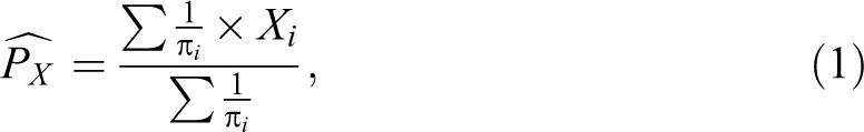
\hat{P_{X}} = \frac{\sum \frac{1}{π_{i}} \times X_{i}}{\sum \frac{1}{π_{i}}},

where π _i is the weight for respondent i. RDS sampling that abides by the original six assumptions is equivalent to the multiplicity sampling that was developed by Sirken (1970; Heckathorn 2007). If the RDS chains are long enough to reach the Markov equilibrium, the probability of inclusion π _i is proportional to i’s degree. Since X_i = 1, if respondent i is a member of group X, and X_i = 0 if i is not a member, then the population proportion of group X can be reduced to:

P_{X}^{VH 2008} = \sum_{i \in X} \frac{1}{d_{i}} / \sum_{i \in \cup (X, Y, Z)} \frac{1}{d_{i}} .

It has been proven that the Volz-Heckathorn (VH) estimator is asymptotically unbiased in sampling systems that exclude the possibility of DRB by limiting each respondent to a single recruitment. The implication is that in this case, the bias approaches zero when the sample size increases (Volz and Heckathorn 2008). Because of the simplicity in the calculation and the estimator’s analytical tractability, the VH2008 estimator has become the most commonly used RDS estimator (Gile and Handcock 2010; Goel and Salganik 2010) despite its inability to control for DRB.

Model-based RDS Estimators

The derivation of the original RDS estimators (Heckathorn 2002, 2007; Salganik and Heckathorn 2004) is based on the “reciprocity model” (Heckathorn 2002), which asserts that the number of cross-group ties on an undirected network should be equal in both directions between any pair of groups, that is T_XY = T_YX, where X, Y denote the initiating and targeting groups. Instead of directly estimating the population proportion from the sample, the model-based approach first infers the cross-group ties and then deduces the population estimate from the network reciprocity equations between each pair of groups. An unacknowledged strength of this model-based approach is that researchers can develop models based on human recruitment behaviors, including the social contexts within which the sampling is conducted, and then infer the cross-group ties based on both recruitment counts in the sample and the model built for the specific population.

In the model-based RDS approach, the number of cross-cutting ties from group X to group Y is a product of four quantities:

T_{X Y} = N P_{X} D_{X} S_{X Y} .

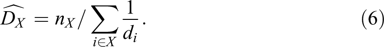
N is the target population size. P_X is the population proportion of group X, which is the variable intended to be estimated. D_X is the average degree of members in group X and S_XY is group X’s proportion of cross-group ties to group Y. The product of the first three terms on the right side of the equation is the total number of ties from group X and multiplying it with the proportion of ties going to group Y yields the number of cross group ties. Because T_XY = T_YX, and given that groups’ proportional sizes sum to one, we can derive the following set of equations for a population of three groups.

\begin{array}{l} 1 = \hat{P_{X}} + \hat{P_{Y}} + \hat{P_{Z}} \\ N \hat{P_{X}} \hat{D_{X}} \hat{S_{X Y}} = N \hat{P_{Y}} \hat{D_{Y}} \hat{S_{Y X}} \\ N \hat{P_{X}} \hat{D_{X}} \hat{S_{X Z}} = N \hat{P_{Z}} \hat{D_{Z}} \hat{S_{Z X}} \\ N \hat{P_{Y}} \hat{D_{Y}} \hat{S_{Y Z}} = N \hat{P_{Z}} \hat{D_{Z}} \hat{S_{Z Y}} . \end{array}

The terms to be estimated are given hats. Solving the equations for $\hat{P}$ is dependent on two estimated quantities: the mean degree of group members, $\hat{D}$ , and the proportion of cross-group ties, $\hat{S}$ . The mean degree for a group is estimated using multiplicity estimation, which uses the harmonic mean of the sampled respondents who are members of the group in question:

\hat{D_{X}} = \frac{\sum \frac{1}{π_{i}} \times d_{i}}{\sum \frac{1}{π_{i}}},

where π _i is the probability of inclusion for respondent i in the sample. When the sampling process reaches the Markov equilibrium, the inclusion probability is proportional to the degree of the respondent, such that π _i = d_i . Substituting this into the equation, we get:

\hat{D_{X}} = n_{X} / \sum_{i \in X} \frac{1}{d_{i}} .

In Heckathorn (2002, 2007) and Salganik and Heckathorn (2004), $\hat{S_{X Y}}$ is estimated as the proportion of recruitments radiating from group X to Y out of the total number of recruitments by X, that is $\hat{S_{X Y}} = R_{X Y} / R_{B X}$ , where $R_{B X} = R_{X X} + R_{X Y} + R_{X Z}$ , an estimate which was shown to be unbiased when the assumptions of the model are met (Salganik and Heckathorn 2004:214). The estimation of $\hat{S_{X Y}}$ based on the outbound recruitments from group X is illustrated in Figure 1, which shows that the total recruitments by X is the sum of the number of recruitments directing from group X to groups X, Y, and Z. In the original formulation, the S matrix is then estimated by the transition matrix, with each cell equal to the proportion of recruitment ties emanating from each recruiting group to each respective recruited group.

[\begin{matrix} S_{X X} & S_{X Y} & S_{X Z} \\ S_{Y X} & S_{Y Y} & S_{Y Z} \\ S_{Z X} & S_{Z Y} & S_{Z Z} \end{matrix}] = [\begin{matrix} \frac{R_{X X}}{R B_{X}} & \frac{R_{X Y}}{R B_{X}} & \frac{R_{X Z}}{R B_{X}} \\ \frac{R_{Y X}}{R B_{Y}} & \frac{R_{Y Y}}{R B_{Y}} & \frac{R_{Y Z}}{R B_{Y}} \\ \frac{R_{Z X}}{R B_{Z}} & \frac{R_{Z Y}}{R B_{Z}} & \frac{R_{Z Z}}{R B_{Z}} \end{matrix}] .

Figure 1.

Recruitment counts among three groups.

One strength of the above estimation, as discussed in detail in Heckathorn (2002:21), is that it depends not on the absolute number of recruits but rather on the proportional distribution of recruits. Therefore, the bias introduced by certain recruitment behaviors, such as one group recruiting more effectively than other groups, does not affect the equilibrium.

In addition, if there exists more than two groups in the population, the set of equations is overdetermined, meaning that the number of equations exceeds the number of unknowns ( P ). The problem is solved based on two model-based transformations of the transition matrix (Heckathorn 2002, 2007). First, in each row of the transition matrix, the cells are multiplied by the equilibrium proportion of the respective group and the total sample size. The resultant term, $S_{X Y} E_{X} R B$ (E_X is the equilibrium proportion of group X and RB is the total number of recruits.), is the expected number of recruits of group X by group Y had both groups recruited with equal success. This step is called demographic adjustment or “raking.” The transformed recruitment matrix is then smoothed by replacing the XY and YX cells by their average value. The resultant smoothed recruitment matrix is “reciprocity compatible” (Heckathorn 2007:174). It solves the overdetermination problem because the excess equations become redundant. This step is called data smoothing. In summary, the solution to the problem of overdetermination is to reduce the number of equations by modeling the reciprocal property of the social network. This modeling approach has a beneficial effect with respect to the variability of estimates, because the cross-recruitment terms are reduced in number by half, and each is then calculated using, ceteris paribus, twice as much data. For example, after data smoothing, R_XY and R_YX are rendered equal, and each term is calculated from data for both R_XY and R_YX _.

Model-based Estimation and Differential Recruitment

RDS is entirely directed by respondents after initial seeds are selected by administrators, therefore it is difficult to monitor or control the sampling process if respondents with varied characteristics behave differently when recruiting the next wave of respondents. Differential recruitment is a broadly defined process that gives rise to the biased sample composition due to systematic differences in recruitment behavior across groups. Because the recruitment process is hidden and the only information that researchers can access is the sample chains and respondents’ surveys, it could be fruitful not to restrict the definition of differential recruitment to a narrow set of behavioral mechanisms. Other behavioral mechanisms in varied social contexts can be found in other RDS studies. Prior work on RDS (Heckathorn 2002, 2007) has recognized differential recruitment as an important source of bias in the sample, and techniques have been developed to adjust for its influence on population estimates.

Two criteria were suggested as a means to detect differential recruitment in the sample (Heckathorn 2007): differential recruitment effectiveness (DRE) and differing recruitment patterns (DRP). Differential recruitment effectiveness refers to the differences in the probability that a coupon passes on to a respondent’s potential recruits in the next wave.² We can identify whether there is differential effectiveness by examining the recruitment matrix:

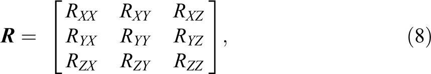
R = [\begin{matrix} R_{X X} & R_{X Y} & R_{X Z} \\ R_{Y X} & R_{Y Y} & R_{Y Z} \\ R_{Z X} & R_{Z Y} & R_{Z Z} \end{matrix}],

where R_XY is the number of recruitments by group X of group Y. In the matrix, the row sum of group X, $R B_{X} = R_{X X} + R_{X Y} + R_{X Z}$ , represents the total number of recruitments by group X, and the column sum, $R O_{X} = R_{X X} + R_{Y X} + R_{Z X}$ , represents the total number of recruits of group X. An unbiased RDS sample should demonstrate equality between the row sums and the column sums. In the NY Jazz study (Heckathorn and Jeffri 2003), the row sum for the non-Hispanic white group (Table 1) is 144 (= 94 + 32 + 18), and the column sum for the non-Hispanic white group is 134 (= 94 + 29 + 11), so white respondents in the sample are overrepresented. The recruitment effectiveness of the white group is 144/134 (i.e., $R B_{X} / R O_{X}$ ), and the recruitment effectiveness of the non-Hispanic black group is 78/81. On average, white respondents are 1.12 times, (144/134)/(78/81), more effective in recruitment than black respondents. Applying the same calculation to the Hispanic group, we know that white respondents are 1.40 times more effective in recruitment than Hispanic respondents.

Table 1.

Recruitment Matrix by Racial Groups in the New York Jazz Study.

	White	Black	Hispanic	Row Sum
White	94	32	18	144
Black	29	41	8	78
Hispanic	11	8	4	23
Column Sum	134	81	30	245

Differing recruitment patterns (DRPs) refer to how (and if) the composition of recruits differs between groups. In the recruitment matrix, we can examine whether one group, for example, Y, is proportionally over/underrepresented in group X’s recruits (i.e., $R_{X Y} / R B_{X}$ ) compared to Y in group Y’s recruits (i.e., $R_{Y Y} / R B_{Y}$ ). Again, an RDS sample from a network characterized by random mixing (i.e., zero homophily) should reflect equality between these two terms, with differences that reflect only stochastic variation in the recruitment process. In the NY Jazz study, among the set of respondents who were recruited by whites, 22 percent (i.e., 32/144) are black, while among the set of the respondents who were recruited by blacks, 53 percent (41/78) are black. Black respondents recruited disproportionately more black individuals than respondents from other racial groups. This recruitment pattern reflects homophily, not random mixing.

If both criteria are identified in the recruitment matrix, the sample may produce inaccurate estimates of populations due to DRB. However, this bias does not arise if either of these two conditions is absent in the sample. For instance, if all groups recruit with differential effectiveness, that is $R B_{X} \neq R O_{X}$ , but the recruitment patterns are identical in all the groups, then the DRB does not arise. In essence, if all groups recruit using an identical pattern, it does not matter which groups recruit more than their peers or less than their peers.³

Alternatively, if groups are equally effective in recruitment, but in the sample, the recruitment patterns are different, for example, the proportion of ethnic Hispanic respondents being recruited differs by group, the generated RDS sample will also fail to exhibit a DRB, because irrespective of differing levels of homophily, the row sums of the recruitment matrix (i.e., RB), and the column sums (RO), will be equal. Hence, the sample composition will correspond to the Markov equilibrium.

For analytical clarity, it is useful to decompose recruitment effectiveness into two behavioral sources: the effectiveness of distributing coupons (U) from the initiating group to the targeting group, that is, the extent to which the coupons given to the recruiter will be passed to the recruit, and the nonparticipation (V) from the targeting groups after the coupons are received, that is, the probability that the coupon will be discarded instead of used to enroll in the study. We define recruitment attempts as coupons that are sent to the recruits, while those coupons are given to the recruiters but not sent out are not considered as attempts. We denote recruitment attempts as A_XY (from group X to Y) and A_X (from group X). Only a fraction 1 − V of the recruitment attempts is realized in the sample (R), therefore the recruitment attempt between any two groups can be estimated with the information of the recruitment relationship in the sample and the nonparticipation rate obtained from the post-RDS survey. Formally,

A_{X Y} = \frac{R_{X Y}}{1 - V_{Y X}},

where V_YX means the participation rate of group Y when the coupons are received from group X. Therefore, we can arrive at the matrix of recruitment attempt A .

A = [\begin{matrix} \frac{R_{X X}}{1 - V_{X X}} & \frac{R_{X Y}}{1 - V_{Y X}} & \frac{R_{X Z}}{1 - V_{Z X}} \\ \frac{R_{Y X}}{1 - V_{X Y}} & \frac{R_{Y Y}}{1 - V_{Y Y}} & \frac{R_{Y Z}}{1 - V_{Z Y}} \\ \frac{R_{Z X}}{1 - V_{X Z}} & \frac{R_{Z Y}}{1 - V_{Y Z}} & \frac{R_{Z Z}}{1 - V_{Z Z}} \end{matrix}] .

In the original formulation of the reciprocity model (equation 4), recruitment counts between groups are used for the estimation of the cross-group transition probability ( S ), that is, the group X’s proportion of network ties radiating to group Y. While given that there is a nonzero and nonuniformly distributed participation rates across groups, the recruitment attempt ( A ) becomes the better term to estimate the cross-group ties. So the proportion of cross-group ties can be estimated as the group X’s proportion of recruitment attempts to Y, as following:

\hat{S_{X Y}} = \frac{A_{X Y}}{A_{X}} = \frac{\frac{R_{X Y}}{1 - V_{Y X}}}{\frac{R_{X X}}{1 - V_{X X}} + \frac{R_{X Y}}{1 - V_{Y X}} + \frac{R_{X Z}}{1 - V_{Z X}}},

When one group’s effectiveness of distributing coupons is the same across groups, that is, $U_{X} = U_{X X} = U_{X Y} = U_{X Z}$ , the U terms will not affect the equation (11). The implication is important in that as long as recruitments of each group are consistent, the differential effectiveness of recruitment for different groups (e.g., $U_{X} \neq U_{Y}$ ) does not affect the recruitment transition probability S .

If there is no systematic variation in participation across all groups as well, then the right side of the equation can be reduced to the original definition of transition probability, in which the nonparticipation was assumed to be none:

\hat{S_{X Y}} = R_{X Y} / R B_{X} .

The strength of rewriting the recruitment matrix as the equation (10) is that it allows the inference to take into account the additional information about the context within which the RDS is conducted. In the following sections, we exemplify it with three elaborated scenarios where the participation rate varies, namely, by the effectiveness of coupon distribution, by nonparticipation, and by intergroup tension. We report results of the model-based and design-based estimators based on the simulated samples that are gathered from these specified settings.

Design of the Study

We use a hypothetical population composed of three groups, infected, uninfected, and recovered, with sizes 1,000, 1,000, and 3,000, respectively. Each of the groups is constructed using the BA network generator (Barabasi and Albert 1999) which allows the degree distribution to resemble the power-law distribution in real social networks. The mean degrees of three groups are 200, 200, and 80.⁴ Then we apply a double-edged swap procedure to induce varied levels of homophily in the system (McPherson, Smith-Lovin and Cook 2001). The double-edged swap procedure first finds two random pairs of connected nodes, removes the edges among them, and then creates new edges between nodes that were previously unconnected in that pair. This breaks down the level of connections between nodes from the same group and increases the randomness in the network connections. The advantage of the procedure is that it holds the degree distribution constant throughout the rewiring process. As the number of swaps increases, the network becomes less homophilous in terms of group status, and it becomes completely mixed when the rewiring procedure runs for an infinite amount of time.

Six seeds are randomly selected in the population. Every recruiter is randomly given either 1 or 2 coupons randomly, unless the number of coupons for the particular group is under examination. Every coupon can be used to recruit one person. To be consistent with the sampling fractions that are most frequently observed in various RDS studies, we use a 5 percent sampling fraction in the simulated RDS process. The recruitment is without replacement.

Results

Effectiveness of Coupon Distribution

Effectiveness of coupon distribution refers to the extent to which coupons successfully pass to another person. The population estimate could be biased if one group is systematically more effective in distributing coupons than other groups ( $U_{X} \neq U_{Y}$ ). While the tendency of nonparticipation may vary across groups after the coupons are received, we isolate the coupon distribution rate by holding the nonparticipation constant. In this section, the main objective is to compare the model-based estimator from Salganik and Heckathorn (2004; ModelSH in Figure 2), with the design-based estimator from Volz and Heckathorn (2008; DesignVH in Figure 2), in the condition where the effectiveness of distributing coupons differs between groups. This test speaks directly to the ongoing debate about the DRB in the RDS studies (e.g., Tomas and Gile 2011).

Figure 2.

Performance of the naive estimator, design-based estimator (DesignVH), and model-based estimator (ModelSH) under the conditions where homophily and recruitment effectiveness vary.

Early model-based estimators (Heckathorn 2002; Salganik and Heckathorn 2004) estimate the proportion of cross-group ties ( S ) using the number of recruitment relationships between groups. If the effectiveness of coupon distribution for one group (e.g., X) is doubled, such that U_XY and U_X increase to 2U_XY and 2U_X, then the group’s effective cross-group recruitment of Y (R_XY) and the group’s total number of recruits (R_BX) will also be doubled. Therefore, the estimate of S remains constant, and the estimator based on the reciprocity model should adjust the differential recruiting effectiveness perfectly.⁵

In the simulation, we assume that every person who receives a coupon participates in the simulation study, and group X’s effectiveness in distributing coupons is operationalized as the number of coupons assigned and the distribution effectiveness for the other two groups remains in the baseline condition for different treatments for group X. Three levels of differential effectiveness are considered. One where members successfully distribute one or two coupons randomly (baseline condition), one where members successfully distribute three coupons (moderate differential effectiveness) and another where members successfully distribute four coupons (high differential effectiveness). Homophily in the network is measured by the dual homophily, a variant of Coleman’s homophily measure.⁶ It takes account of both cross-group ties and groups’ mean degrees. We also divide the homophily continuum to three categories: zero homophily, moderate homophily, and high homophily. Figure 2 shows the performance of estimators across the nine different pairings of differential effectiveness (grouped by column) and network homophily (grouped by row).

When the network is randomly mixed, a difference in the coupon distribution effectiveness has no effect on the estimation. Both the design-based (DesignVH) and model-based estimators (ModelSH) perform equally well, and estimates coincide with the true proportion (0.2, the horizontal line) covered by the confidence intervals. The naive estimator, on the other hand, deviates from the true population proportion. As the homophily in the network increases from zero to moderate, the VH estimator begins to overestimate the population proportion when there is some differential effectiveness of coupon distribution, while ModelSH remains close to the true proportion. As homophily further increases, the performance difference between the design-based and model-based estimators becomes even larger. The estimators based on the reciprocity model produce an unbiased estimation of the population proportion when both homophily and differential distribution effectiveness are present. The results are consistent with the predicted differences between the DesignVH and ModelSH estimators that are illustrated in the hypothetical example in Table 1.

Nonparticipation

Nonparticipation (nonreturn) refers to the potential for a recruit to choose not to participate in the study after receiving a coupon (Gile, Johnston, and Salganik 2015; Tomas and Gile 2011). To avoid the misuse of terminology and to be consistent with the literature (Gile, Johnston, and Salganik 2015), we refer to nonparticipation as one of the two types of general nonresponse in RDS. Another type is declining to accept coupons, or so-called coupon refusal by Gile, Johnston, and Salganik (2015; Iguchi et al. 2009). While both types of nonresponse need to be taken into account in the estimation of population composition, the latter type (coupon refusal) can be easily identified with a post-RDS survey of respondents who can describe the characteristics of people who refuse to accept coupons. Then the RDS-inferred population proportion will be divided by the factor of coupon giving rate, that is, coupons received by the group divided by coupons given to the group. The segment of the population that refuses to accept coupons does not influence the subsequent recruitment dynamics. However, the former type (nonparticipation) is more difficult to control because those who accept the coupons but do not participate can alter the dynamics of the subsequent RDS chains, and therefore affect the sample composition. A simple weighting of the population estimate cannot solve the underrepresentation problem. We adjust the rate of nonparticipation using the model formulated in equation (10).

RDS respondents have shown high nonparticipation rates in the studies that had implemented post-RDS surveys inquiring about respondents’ recruitment behaviors. In a 12-site RDS study in the Dominican Republic, nonparticipation rates ranged from 13.4 percent to 44.6 percent in different sites. The rate was slightly higher among female sex workers than IDUs and MSMs (Gile, Johnston, and Salganik 2015). Yamanis et al. (2013) also differentiated three types of network alters: those who were invited and accepted the invitation to participate, those who were invited but refused to participate, and those who were not invited to participate. While they didn’t calculate the nonparticipation rate specifically, they compared the population estimates based on the bootstrapped samples using the actual recruitment and the invited network composition. Noticeable differences can be found between the estimates using these two pieces of information. (However, the difference is much smaller compared to the difference between either of them and the estimate calculated using the estimated network composition by the respondents.)

One important source of nonparticipation comes from the suitability of the population to RDS. If one group systematically chooses not to participate, or cannot access the interview site conveniently, the nonparticipation bias can lead to biased RDS estimation. For instance, in an RDS study of a rural Ugandan population (McCreesh et al. 2011), villagers who lived more than 1 km away from the nearest interview site were less likely to be recruited than those living within a 1 km range. Furthermore, respondents who lived 1 km away from the interview site were much less likely to participate in the study if they didn’t have a car or motorcycle in their household. Therefore, people living in distant villages were undersampled. Another example of the research design leading to bias is the choice of the location of the interview site in the study of IDUs in Bridgeport, CT (Heckathorn 2008). At first, the interview site was located in a predominately African American neighborhood where RDS yielded a sample that overrepresented African Americans compared to their self-reported network composition, which was a mix of African Americans and Hispanics. Hispanics were reported by respondents to be unwilling to participate in the study because they were not comfortable in the interview site’s location. After the interview site was moved to neutral ground where both groups had easy and comfortable access, the proportion of Hispanics in the sample increased significantly. All these conditions can cause low response rates for particular groups in the RDS study.

To account for the systematic bias for or against a particular group (e.g., group X), we set the deviance of the nonparticipation rate to be identical for all recruitment attempts directed to that group. For instance, if group X suffers from impediments preventing them from participating in the study, their nonparticipation rates to every other group will be positive and identical, that is, $V_{X X} = V_{Y X} = V_{Z X} > 0$ .

For simplicity, in the simulation, we only vary the nonparticipation rate of group X. In our model, groups Y and Z respond fully to the received coupons. The nonparticipation rate V_X is set to four values: zero (V_X = 0), low (0.2), moderate (0.4), and high (0.8). In Figure 3, we group nonparticipation rates by column and network homophily by row. The variant of the model-based estimator that adjusts for nonparticipation bias is named as ModelNP in Figure 3, a variant that uses group-specific response rates (i.e., V) in the adjusted recruitment matrix (equation 10). It is compared with the naive estimator (sample proportion) and DesignVH estimators in Figure 3.

Figure 3.

Performance of the naive estimator, design-based estimator (DesignVH), and model-based estimator that has controlled for nonparticipation behavior (ModelNP) under the conditions where homophily and nonparticipation rate vary.

All three estimators perform equally well when there is no nonparticipation bias for group X (the left column). However, when the nonresponse rate increases to 20 percent, DesignVH underestimates the population proportion, while the estimator based on the adjusted model correctly estimates the population proportion. As the underlying network becomes more homophilous, the deviance of DesignVH from the true population proportion becomes larger. However, the median of ModelNP remains relatively the same as the network changes from randomly mixed (zero homophily) to highly homophilous and the recruitment effectiveness from low to high, except for the case where both high different effectiveness of recruitment and high homophily are present in the system (upper right corner in Figure 3). We recommend that a population with high homophily among groups and very high nonparticipation is not suitable to RDS study, as the variance of the estimate becomes too large to be useful for any practical use. For the rest of the combinations, the noticeable trend for ModelNP is an increasingly widening confidence interval as both dimensions in Figure 3 increase. In the last column, the nonparticipation rate increases to 80 percent, and the pattern of the difference present in the 20 percent nonparticipation condition becomes even more pronounced.

Intergroup Status Difference

Social groups characterized by distinctive traits and social boundaries commonly held by members sometimes show in-group favoritism and out-group hostility (Tajfel 1982; Tajfel and Turner 1979). Recruitment attempts from an out-group member are likely to be refused or discarded when intergroup tension is present. The relationship between groups becomes particularly crucial for RDS if the out-group perception between two groups is asymmetric.⁷ For instance, it is common that low-status groups favor interaction with high-status groups, but the reverse is not the case. In an RDS study that crosses different sociodemographic strata, people from high-status groups, for example, white-collar workers, may be less likely to respond affirmatively to coupon offers from members of low-status groups, such as people living on the streets.

The operational difference between the biases caused by intergroup status difference and by nonparticipation is that the perceived status difference between groups is placed on out-group members rather than on in-group members, while the mechanism of nonparticipation is systematically uniform for everyone in the group due to their commonly perceived impediment (e.g., distant location or perceived danger). We use a similar strategy to update the recruitment matrix by the adjusted recruitment matrix (equation 10), with only selected pairings of groups having their nonparticipation rates deviate from other groups.

A partial solution to this problem arises due to the scalar nature of the U.S. stratification system. Rather than a caste-like separation, individuals are ranged along a continuum from very low status to very high status, with each individual tending to associate with those at their own level, and also those a bit higher and a bit lower. This provides the potential for recruitment chains to travel incrementally, from low- to high-status respondents. For example, in the Ramirez-Valles et al. (2005) study of Latino MSM, recruitment from the lowest income quintile to those in the highest quintile of income was rare, but low-income respondents sometimes recruit those with modestly higher income, these in turn recruit those who are even more affluent, so chains can expand from lower to higher points in the stratification system.

In the simulation, we now try to vary group X’s nonparticipation rate by the group where the recruiter is from. We set V_XX = 1, V_YX = 0.6, and V_ZX = 0.6, meaning that group X sometimes refuses recruitment overtures only to out-groups, Y and Z, but not the recruitment attempts from its own group. The new variant of the model-based estimator is named ModelST in Figure 4, and it is compared with the naive estimator and DesignVH in Figure 4. We also vary the network homophily and compare the performance of these estimators under different network conditions.

Figure 4.

Performance of the naive estimator, design-based estimator (DesignVH), and model-based estimator that has controlled for intergroup status difference (ModelST) under the conditions where homophily varies.

When the network is randomly mixed by group status, both DesignVH and H2007 estimators underestimate the population proportion, but the adjusted “status” estimator, which has accounted for the nonparticipation rate in the transition matrix, performs relatively better, with the interquartile range (the “whisker box”) covering the true population proportion. As the network becomes more homophilous on the group status, the confidence interval becomes wider for all estimators, but the whisker box for the ModelST estimator consistently contains the true population proportion.

Rules for Detecting Differential Recruitment Bias

The causes of differential recruitment are likely complex and hidden to researchers. Based on the results obtained from simulated samples, we suggest the following rules for detecting DRB in the RDS study.

1. Post-RDS survey

A post-RDS survey of respondents who have participated in the study and returned to receive rewards for peer recruitment is a useful way to detect a difference in responding behavior between groups (Gile, Johnston, and Salganik 2015; Iguchi et al. 2009). A proper question to ask in the post-RDS survey, following the recommended interview question by Gile, Johnston, and Salganik (2015), could be “among all three coupons given to you, how many did you distribute to group X (Y and Z)?” By aggregating the distributed coupons over members of a particular group (e.g., X), we can get the counts of attempted recruitments from group X of each of the groups in the post-RDS survey (denoted as PA_XY). The proportion of RDS respondents who are surveyed in the post-RDS survey is $\frac{F}{R}$ , where F is the number of surveyed respondents and R is the RDS sample size. So the estimated attempted recruitments from group X of Y is $\frac{P A_{X Y} \times R}{F}$ . Using the resultant RDS sample, we can know the realized recruitments from X to Y as R_XY. So reversing the equation (9), we can arrive at the estimated nonparticipation rate of group Y when coupons are from group X: $V_{Y X} = 1 - \frac{R_{X Y} \times F}{P A_{X Y} \times R}$ .

2. Examining the Recruitment Matrix

RDS samples provide important information about whether the sampling process is affected by differential recruitment behavior. The main source of DRB is from the interaction of differing effectiveness of recruitment and homophily in the network structure. The pattern is most evident in Figure 2, where the model-based estimators are superior to the design-based estimator when both differential recruitment effectiveness and homophily are relatively high. Information in the sample provides a useful approximation of both the respondents’ behaviors and the network structure. Heckathorn (2007) suggested two practical rules for detecting DRB, which resulted from two distinct recruitment behaviors: differential effectiveness of recruitment and differing recruitment patterns. The former can be evaluated by comparing the row sum (recruitment count by a group) and the column sum (recruitment count of a group) in the recruitment matrix. When the row sum and column sum are largely different, we should suspect that one group recruits more effectively. With the simulated sample, we derive the following convenient formula to calculate the average difference across groups.

Diff = \frac{1}{g} \sum_{X \in g} \frac{| {rowsum}_{X} - {colsum}_{X} |}{{rowsum}_{X} + {colsum}_{X} / 2} .

The second practical rule suggested in Heckathorn (2007) is to examine whether or not there are differing patterns of recruitment in the sample, which is the difference in the recruits’ composition across groups. Differing recruitment patterns have several causes, the most robust cause is homophily in the network. When homophily is present in the network, we would expect to find a disproportionately high number of within-group recruitments.

In Figure 5, we plot the differing recruitment effectiveness measured by equation (13) on the horizontal axis, and the homophily in the sample measured by the Coleman homophily index on the vertical axis. Each dot represents a single RDS-simulated sample that was pulled from the first experiment. Dots are colored by the difference between the performance of VH and SH2004 with respect to the true population proportion. Written formally, it is $| P_{X}^{VH} - P_{X}^{true} | - | P_{X}^{SH 2004} - P_{X}^{true} |$ , where $P_{X}^{true}$ is the true population proportion. When there is no difference between the design-based and model-based estimators, the dots are colored light yellow. As the difference increases from zero, the dot becomes darker, and the dots are colored a dark orange when the difference is at its maximum observed value. We drew a line extending from the x-axis to the y-axis, differences between estimators on the lower left-hand side of this line are negligible. As a suggestion for researchers, we recommend computing the homophily and the difference between row sum and column sum with values from the recruitment sample and then decide whether or not additional modeling is required for estimation.

Figure 5.

Difference of bias between DesignVH and ModelSH estimators by homophily in the recruitment ties and differential effectiveness of recruitment in the sample.

Conclusion

A common criticism of RDS is that it depends for its validity on multiple assumptions which frequently do not hold in the field. In this article, we examined two types of RDS estimator, a model-based approach, which is based on models of human recruitment behavior and the social context within which sampling is conducted, and a design-based approach, which relies on the known probability of selection in sampling. We showed that a distinctive advantage of the model-based approach is that the model, when suitably constructed, provides the means for controlling for sources of bias which escape the design-based approach.

Three means for controlling bias were discussed in this article. The first, built into the SH2004 estimator, controls for DRB resulting from the combination of differential recruitment effectiveness (DRE) and differing recruitment pattern (DRP). The second that was proposed in this article (ModelNP) is an estimator that controls for bias from what we term “nonparticipation” in which a respondent accepts a recruitment coupon but then decides not to participate in the study. The third, which was also proposed in this article (ModelST), controls for bias when status differences induce asymmetries in the recruitment patterns.

These three examples serve as illustrations of a paradigm for reducing the dependence of an RDS estimator on counterfactual assumptions. Given the marvelous flexibility of mathematical models, we anticipate that in future papers, this approach can be employed in other contexts to provide a family of RDS estimators which are, in combination, less dependent on counterfactual assumptions.

A design-based estimator, it should be noted, can also be adjusted to reduce its dependence on counterfactual assumptions. A notable example is Thompson’s (2006) targeted random walk design. As he notes, a limitation of a traditional random walk design is that the stationary distribution frequently does not reflect the distribution of the population from which the sample was drawn. He proposes several means by which the walk is “nudged” (p. 11), for example, so that one could sample IDUs with twice the probability of other nodes, or one could draw a sample where the probability of inclusion is proportional to a node’s out degree. This is an elegant mathematical demonstration of the range of possible random walks, and hence a useful contribution to the theoretic literature on random walks. The aim of this article does not appear to include proposing a sampling method, which might be applicable in the field, for example, it is not clear how one might nudge a population of drug users to recruit peers based on factors that may not be public knowledge, such as a node’s out degree. This illustrates an important difference between adjustments for bias in a model-based versus a design-based sampling method. Given the marvelous flexibility of mathematics, the range of potential adjustments in a model-based estimator is very large, even if it requires gathering modest amounts of additional information during the sampling process. In contrast, adjustments to a design-based estimator may require changing the behavior of recruiters in the random walk. Hidden populations such as IDUs have limited tractability with respect to “nudging” their recruitment behavior.

In sum, the model-based approach to RDS statistical inference provides a flexible and potentially more accurate way to account for the behavioral biases in recruitment. The model-based RDS inference method outlined in this article can provide a paradigm for adjusting RDS model-based inference across a wide range of hidden populations, in which special conditions need to be adjusted and modeled.

Footnotes

Acknowledgments

We thank Antonio Sirianni for helpful comments and advice.

Declaration of Conflicting Interests

The author(s) declared no potential conflicts of interest with respect to the research, authorship, and/or publication of this article.

Funding

The author(s) disclosed receipt of the following financial support for the research, authorship, and/or publication of this article: This research was made possible by a grant from the National Institutes of Health/National Institute for Nursing Research (1R21NR10961).

Notes

References

Abdul-Quader

Abu S.

Heckathorn

Douglas D.

McKnight

Courtney

Bramson

Heidi

Nemeth

Chris

Sabin

Keith

Gallagher

Kathleen

Jarlais

Don C. Des

. 2006. “Effectiveness of Respondent Driven Sampling for Recruiting Drug Users in New York City: Findings from a Pilot Study.” Journal of Urban Health 83:459–76.

Barabasi

Albert-László

Albert

Réka

. 1999. “Emergence of Scaling in Random Networks.” Science 286:509–12.

Barash

Vladimir

Cameron

Chris

Spiller

Michael

Heckathorn

Douglas D.

. 2016. “Respondent-driven Sampling—Testing Assumptions: Sampling with Replacement.” Journal of Official Statistics 32:29–73.

Bernhardt

Annette

Milkman

Ruth

Theodore

Nik

Heckathorn

Douglas

Auer

Mirabai

DeFilippis

James

González

Ana Luz

Narro

Victor

Perelshteyn

Jason

Polson

Diana

Spiller

Michael

. 2009. Broken Laws, Unprotected Workers: Violations of Employment and Labor Laws in America’s Cities. Retrieved from http://www.russellsage.org/awarded-project/broken-laws-unprotected-workers-violations-employment-and-labor-laws-americas-cities

Deiss

Robert

Brouwer

Kimberly C.

Loza

Oralia

Lozada

Remedios

Ramos

Rebeca

Cruz

Michelle Firestone

Patterson

Thomas L.

Heckathorn

Douglas D.

Frost

Simon

Strathdee

Steffanie A.

. 2008. “High-risk Sexual and Drug Using Behaviors among Male Injection Drug Users Who Have Sex with Men in 2 Mexico–US Border Cities.” Sexually Transmitted Diseases 35:243–49.

Frost

Simon D. W.

Brouwer

Kimberly C.

Cruz

Michelle A. Firestone

Ramos

Rebeca

Ramos

Maria Elena

Lozada

Remedios M.

Magis-Rodriguez

Carlos

Strathdee

Steffanie A.

. 2006. “Respondent-driven Sampling of Injection Drug Users in Two U.S.-Mexico Border Cities: Recruitment Dynamics and Impact on Estimates of HIV and Syphilis Prevalence.” Journal Urban Health 83:i83–97.

Gile

Krista

Handcock

Mark S.

. 2010. “Respondent-driven Sampling: An Assessment of Current Methodology.” Sociological Methodology 40:285–327.

Gile

Krista

Handcock

Mark S.

. 2015. “Network Model-assisted Inference from Respondent-driven Sampling Data.” Journal of the Royal Statistical Society: Series A (Statistics in Society) 178:619–39.

Gile

Krista J.

Johnston

Lisa G.

Salganik

Matthew J.

. 2015. “Diagnostics for Respondent-driven Sampling.” Journal of the Royal Statistical Society: Series A 178:241–69.

10.

Goel

Sharad

Salganik

Matthew J.

. 2010. “Assessing Respondent-driven Sampling.” Proceedings of the National Academy of Sciences 107:6743–47.

11.

Hansen

Morris H.

Madow

William G.

Tepping

Benjamin J.

. 1983. “An Evaluation of Model-dependent and Probability-sampling Inferences in Sample Surveys.” Journal of the American Statistical Association 78:776–93.

12.

Heckathorn

Douglas D.

1997. “Respondent Driven Sampling: A New Approach to the Study of Hidden Samples.” Social Problems 44:174–99.

13.

Heckathorn

Douglas D.

2002. “Respondent-driven Sampling II: Deriving Valid Population Estimates from Chain-referral Samples of Hidden Populations.” Social Problems 49:11–34.

14.

Heckathorn

Douglas D.

2007. “Extensions of Respondent-driven Sampling: Analyzing Continuous Variables and Controlling for Differential Recruitment.” Sociological Methodology 37:151–207.

15.

Heckathorn

Douglas D.

2008. “Assumptions of RDS: Analytic vs. functional assumptions.” Paper presented at CDC Consultation on the Analysis of Data Collected Through Respondent-driven Sampling, Atlanta, GA.

16.

Heckathorn

Douglas D.

Jeffri

Joan

. 2003. “Finding the Beat: Using Respondent-driven Sampling to Study Jazz Musicians.” Poetics 28:307–29.

17.

Heckathorn

Douglas D.

Wejnert

Cyprian

. 2011. “Distilling the Homophily Concept: Disentangle the Effects of Differentials in Group Size and Network Size from a Measure of In-group Affiliation.” Unpublished mauscript.

18.

Iguchi

Martin Y.

Ober

Allison J.

Berry

Sandra H.

Fain

Terry

Heckathorn

Douglas D.

Gorbach

Pamina M.

Heimer

Robert

Kozlov

Andrei

Ouellet

Lawrence J.

Shoptaw

Steven

Zule

William A.

. 2009. “Simultaneous Recruitment of Drug Users and Men Who Have Sex with Men in the United States and Russia Using Respondent-driven Sampling: Sampling Methods and Implications.” Journal of Urban Health 86:5–31.

19.

Johnston

Lisa Grazina

Khanam

Rasheda

Reza

Masud

Khan

Sharful Islam

Banu

Sarah

Alam

Md. Shah

Rahman

Mahmudur

Azim

Tasnim

. 2008. “The Effectiveness of Respondent Driven Sampling for Recruiting Males Who Have Sex with Males in Dhaka, Bangladesh.” AIDS and Behavior 12:294–304.

20.

Johnston

L. G.

Sabin

Mai

T. H.

Pham

T. H.

. 2006. “Assessment of Respondent Driven Sampling for Recruiting Female Sex Workers in Two Vietnamese Cities: Reaching the Unseen Sex Worker.” Journal of Urban Health 83:i16–28.

21.

McCreesh

Johnston

L. G.

Copas

Sonnenberg

Seeley

Hayes

R. J.

Frost

S. D.

White

R. G.

. 2011. “Evaluation of the Role of Location and Distance in Recruitment in Respondent-Driven Sampling.” International Journal of Health Geographics. doi:10.1186/1476-072X-10-56.

22.

McPherson

Miller

Smith-Lovin

Lynn

Cook

James M.

. 2001. “Birds of a Feather: Homophily in Social Networks.” Annual Review of Sociology 27:415–44.

23.

Millett

G. A.

Ding

Lauby

Flores

Stueve

Bingham

Carballo-Dieguez

Murrill

Liu

K. L.

Wheeler

Liau

Marks

. 2007. “Circumcision Status and HIV Infection among Black and Latino Men Who Have Sex with Men in 3 US Cities.” Journal of Acquired Immune Deficiency Syndromes 46:643–50.

24.

Montealegre

J. R.

Risser

J. M.

Selwyn

B. J.

McCurdy

S. A.

Sabin

. 2013. “Effectiveness of Respondent Driven Sampling to Recruit Undocumented Central American Immigrant Women in Houston, Texas for an HIV Behavioral Survey.” AIDS and Behavior 17:719–27.

25.

Ramirez-Valles

Jesus

Heckathorn

Douglas D.

Vázquez

Raquel

Diaz

Rafael M.

Campbell

Richard T.

. 2005. “From Networks to Populations: The Development and Application of Respondent-driven Sampling among IDUs and Latino Gay Men.” AIDS and Behavior 9:387–402.

26.

Salganik

Matthew J.

Heckathorn

Douglas D.

. 2004. “Sampling and Estimation in Hidden Populations Using Respondent-driven Sampling.” Sociological Methodology 34:193–239.

27.

Sarndal

Carl-Erik

. 1978. “Design-based and Model-based Inference in Survey Sampling.” Scandinavian Journal of Statistics 5:27–52.

28.

Sarndal

Carl-Erik

. 2010. “Models in Survey Sampling.” Pp. 15–27 in Official Statistics, Methodology and Applications in Honour of Daniel Thorburn, edited by Carlson Nyquist Villani . Sweden: Stockholm University.

29.

Stormer

Ame

Tun

Waimar

Guli

Lisa

Harxhi

Arjan

Bodanovskaia

Zinaida

Yakovleva

Anna

Rusakova

Maia

Levina

Olga

Bani

Roland

Rjepaj

Klodian

Bino

Silva

. 2006. “An Analysis of Respondent Driven Sampling with Injection Drug Users (IDU) in Albania and the Russian Federation.” Journal of Urban Health 83:i73–82.

30.

Sirken

M. G.

1970. “Household Surveys with Multiplicity.” Journal of the American Statistical Association 65:257–66.

31.

Tajfel

Henri

. 1982. Social Identity and Intergroup Relations. Cambridge, MA: Cambridge University Press.

32.

Tajfel

Henri

Turner

John

. 1979. “An Integrative Theory of Intergroup Conflict.” Pp. 33–48 in The Social Psychology of Intergroup Relations, edited by Austin

W. G.

Worchel

. Monterey, CA: Brooks-Cole.

33.

Thompson

Steven K.

2006. “Targeted Random Walk Designs.” Survey Methodology 32:11–24.

34.

Thompson

Steven K.

2012. Sampling. Hoboken, NJ: John Wiley.

35.

Tomas

Amber

Gile

Krista J.

. 2011. “The Effect of Differential Recruitment, Non-response and Non-recruitment on Estimators for Respondent-driven Sampling.” Electronic Journal of Statistics 5:899–934.

36.

Volz

Erik

Heckathorn

Douglas

. 2008. “Probability Based Estimation Theory for Respondent Driven Sampling.” Journal of Official Statistics 24:79–97.

37.

Volz

Wejnert

Cameron

Spiller

Barash

Degani

Heckathorn

D. D.

. 2012. Respondent-Driven Sampling Analysis Tool (RDSAT) Version 7.1. Ithaca, NY: Cornell University.

38.

Wang

Jichuan

Carlson

Robert

Falck

Russel

Siegal

Harvey A.

Rahmen

Ahmmed

Linna

. 2005. “Respondent-driven Sampling to Recruit MDMA Users: A Methodological Assessment.” Drug and Alcohol Dependence 78:147–57.

39.

Wang

Jichuan

Falck

Russel

Linna

Rahman

Ahmmed

Carlson

Robert

. 2007. “Respondent-driven Sampling in the Recruitment of Illicit Stimulant Drug Users in a Rural Setting: Findings and Technical Issues.” Addict Behavior 32:924–37.

40.

Wejnert

Cyprian

. 2009. “An Empirical Test of Respondent-Driven Sampling: Point Estimates, Variance, Degree Measures, and Out-of-Equilibrium Data.” Sociological Methodology 39:73–116.

41.

Yamanis

Thespina J.

Merli

M Giovanna

Neely

William Whipple

Tian

Felicia Feng

Moody

James

Xiaowen

Gao

Ersheng

. 2013. “An Empirical Analysis of the Impact of Recruitment Patterns on RDS Estimates among a Socially Ordered Population of Female Sex Workers in China.” Sociological Methods & Research.