
Abstract
In this article, a numerical method integrated with statistical data simulation technique is introduced to solve a nonlinear system of ordinary differential equations with multiple random variable coefficients. The utilization of Monte Carlo simulation with central divided difference formula of finite difference (FD) method is repeated n times to simulate values of the variable coefficients as random sampling instead being limited as real values with respect to time. The mean of the n final solutions via this integrated technique, named in short as mean Monte Carlo finite difference (MMCFD) method, represents the final solution of the system. This method is proposed for the first time to calculate the numerical solution obtained for each subpopulation as a vector distribution. The numerical outputs are tabulated, graphed, and compared with previous statistical estimations for 2013, 2015, and 2030, respectively. The solutions of FD and MMCFD are found to be in good agreement with small standard deviation of the means, and small measure of difference. The new MMCFD method is useful to predict intervals of random distributions for the numerical solutions of this epidemiology model with better approximation and agreement between existing statistical estimations and FD numerical solutions.
Keywords
Differential equation arises in formulation of many real life and industrial-based dynamical relations that describe growth, transformation, and change of specific dependent and independent mechanisms that may affect the whole system of inquisition. Generally, differential equations are categorized as ordinary differential equations (ODEs) or partial differential equations (PDEs). ODEs are differential equations with only one independent variable that reflected in the denominator expression, while PDEs have two or more independent variables in the system. There are three types of solutions for differential equations, which are exact, analytical, and numerical solutions. Many authors have conducted study on differential equations using vast choices of method. Since exact solutions do not exist for many complex models, closed form and analytical solutions are preferred as second-choice alternative depending on the versatility, practicality, and mathematical severity of the problems. Mohyud-Din, Noor, and Noor (2009) reviewed the applications of the analytical methods of He’s and modified variational iterations, homotopy perturbation, parameter expansion, and exp-function to solve a wide class of nonlinear initial and boundary value problems. Further discussion on such methods is also studied in Mohyud-Din and Ali (2016), Mohyud-Din, Yildirim, and Gulkanat (2012), and Ul Hassan and Mohyud-Din (2016). On the other hand, numerical methods are favored by numerical scientists and engineers due to simpler algorithm and computer-handling operations on complex solutions, less time consumption, and when the exact or analytical solutions of certain models are not yet found.
Finite difference (FD) method is one of established numerical methods to solve differential equations approximately. This method is widely applied in practical mathematical and physical modeling (Karris 2007), numerical analysis/simulation, and discrete domain problems throughout many fields of science, engineering, social science, medicine, and economics. Witnessing continuous demand and progress in these fields, many authors employed FD in their works including on ODEs. Rao and Chakravarthy (2013) presented FD method for singularly perturbed linear second-order differential-difference equations of convection–diffusion type with a shift parameter when the shift is smaller or greater than a perturbation parameter. Moghaddam and Mostaghim (2013) used a new numerical method that depends on FD to provide feasible solution for boundary problem of delayed differential equations of fractional order. In 2014, linear second-order differential-difference equation of convection–diffusion type with singularly perturbed boundary value problem is discussed, where a tridiagonal FD method is introduced with fitting parameter from the theory of singular perturbation (Rao and Chakravarthy 2014). Recent works on the FD method can be found in Liu and Chen (2014), Su, Li, and Ding (2013), and Zhao (2013).
Monte Carlo (MC) method is an eminent statistical modeling method in applied mathematics to develop models of phenomena with unknown probabilistic property. Because of its simplicity and good statistical results, the MC method has become a widespread technique used for doubt quantity. Due to increasing demand of statistical modeling and fast development of technology, MC method is employed with multiprocessor computing system in order to simulate many independent statistical experiments at a time. This progress enables difficult problems of probabilistic nature to be solved using the MC method by direct simulation of the natural probability model as well as to solve deterministic problems that are represented as constructed probability processes. These processes are modeled, and the numerical solutions are framed in the form of statistical estimators of deterministic equations with either random coefficients or random boundary conditions or right sides random (Rubinstein and Kroese 2007). The MC method can also be applied to solve problems in finance, science, engineering, economics, and actuarial mathematics. It can be used to generate random data in behavioral studies as well as to estimate numerical quantities via repeated sampling. Moreover, mathematical algorithms can be randomized using computers to carry out statistical sampling in optimization problems via the MC method.
There are many authors who organized research in parameters estimation of ODEs with MC. Spigler and Zerbetto (2013) studied the oscillatory behavior of tension leg platform offshore structure using MC method, while De Souza, Colaço, and Leiroz (2014) provided MC solution of ODEs from a first law analysis and calculated the stochastic moments. Licea, Villafuerte, and Chen-Charpentier (2013) dealt with Riccati equation that has random coefficients and compared the solutions with MC method. Buezas, Rosales, and Sampaio (2013) solved a nonlinear ODE using finite element method with MC simulation technique. Recently, Leander, Lundh, and Jirstrand (2014) presented an article related to estimated parameters of ODEs that have experimental data for discrete time. It is demonstrated that transforming an ODE to a stochastic differential equation as an objective function eliminates problem of local minima. Rohaninejad and Zarghami (2012) predicted the behavior of impounded dams by employing MC with FD method, where the statistical test Kolmogorov–Smirnov is used to predict the dam behavior. Other applications of MC method are given in Abdulle and Blumenthal (2013), Dereich and Heidenreich (2011), and Kovtanyuk, Botkin, and Hoffmann (2012).
Obesity and overweight are excessive fats in one’s body measured using a simple formula of body mass index (BMI). These abnormal body weights have been medically proven as major risks to modern population with known linkage to many death cases around the world due to cardiovascular diseases, such as stroke and heart disease, diabetes, musculoskeletal disorders especially osteoarthritis, and also due to colon, endometrial, and breast cancers. Based on statistics from the World Health Organization, the world obesity rate has increased by 200 percent since 1980 with 42-million children under five years old are obese or overweight in 2013 alone. Mainly caused by imbalance of daily nutritional intake and lack of physical activities to burn extra calories taken, the excess weight continues to become a serious health problem, especially in the low- and middle-income countries exasperated by insufficient prevention strategies, law policies, and power enforcement by the corresponded governments. As much as the rate of excess weight is rising at worrying stage, the research and studies devoted to this issue also keep rising.
Santonja et al. (2012) studied the effects of a public campaign to reduce excess weight in a Spanish region within a community of Valencia that is caused by unhealthy lifestyles. A mathematical model is presented to track on the progression of excess weight loss influenced by prevention strategy of public health campaigns. The campaigns focus on overweight and/or obese individuals in order to reduce their weight. In Snyder (2007), the author reached to a conclusion that nutritional campaigns should be able to change feeding behavior. Christakis and Fowler (2007) investigated similar issue by assuming the excess weight (obesity and overweight) as a socially transmitted epidemic disease. Further studies on excess weight from diverse perspectives are conducted in Livingston et al. (2001); Navarro-Barrientos, Rivera, and Collins (2011); and Thomas et al. (2014).
In the present study, FD method integrated with MC technique is considered to simulate coefficients of time t (week) of a nonlinear system of equations representing three Valencia community subpopulations based on BMI (Santonja et al. 2012). The system consists of three nonlinear ODEs with multiple coefficients/parameters that are described as random variables with probability distributions. The integrated method we named as mean Monte Carlo finite difference (MMCFD) method is used to simulate the parameters of the model (Santonja et al. 2012) and secondly to calculate the prediction interval for the numerical solution of every dependent variable of the system when the real-valued coefficients are provided previously. Because of random sampling and rounding errors, the solution must be supported by prediction interval based on percentile of variables distribution. In particular, we are using the 5th and 95th percentiles in the present work. This interval of numerical results is later compared with the interval of statistical predictions (Santonja et al. 2012) derived by Latin hypercube sampling (LHS) technique. In order to obtain empirical prediction intervals, this article leads to set up interval by using the percentiles from the simulated values. This predicted interval represents empirical prediction intervals. The MMCFD solutions are also compared with the results generated by the FD method via central divided difference formula. The MMCFD method shows better accuracy and convergence to the given predicted results than the FD method. Thus, it is expected that the MMCFD method has a potential in future estimations with probabilistic model.
Mathematical Model
Consider the epidemiological model of a group of people in the Valencia community of Spain (Santonja et al. 2012) on the effects of public health campaigns toward the community weight loss. The selected group of adults at the age of 23 years old is divided into three subpopulations according to their BMI, which is calculated as BMI = weight/height2:
N—subpopulation of individuals with normal weight (BMI < 25),
S—subpopulation of individuals with overweight (25 ≤ BMI < 30), and
O—subpopulation of individuals with obesity (BMI ≥ 30).
The transition of individual weight is observed at the age of 24 years old in all subpopulations of N, S, and O, which is a year prior to the public health campaign organized in 2000. The initial subpopulations of individuals at the age of 23 years old with normal weight, overweight, and obesity are denoted by


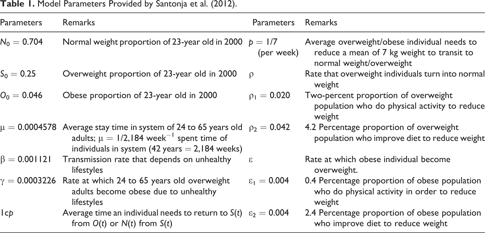
Other parameters of the model (Santonja et al. 2012) are listed in Table 1 with further estimation details. This model is a system of ODEs with variable solutions depending on time t. The model parameters are random variables with estimated values. This is where the MMCFD method can be very useful to solve the model numerically.
Model Parameters Provided by Santonja et al. (2012).
Solution Approach
The general form of a nonlinear initial value problem is written as:

We divide [a, b] into T subintervals such as ti = a + ih for i = 0, 1, 2,…, T, where T is the maximum number of iterations and h is a step size. The step size h = 1 (one week) is chosen here since we are analyzing the actual social epidemic model of body weight change which is more suitable to be observed by weekly at the least instead of by daily. Therefore, the equation (4) becomes:

By using central difference formula of FD method, the equation (5) becomes:

Upon substitution of the equation (6) into the nonlinear system of ODEs (1) to (3) gives:


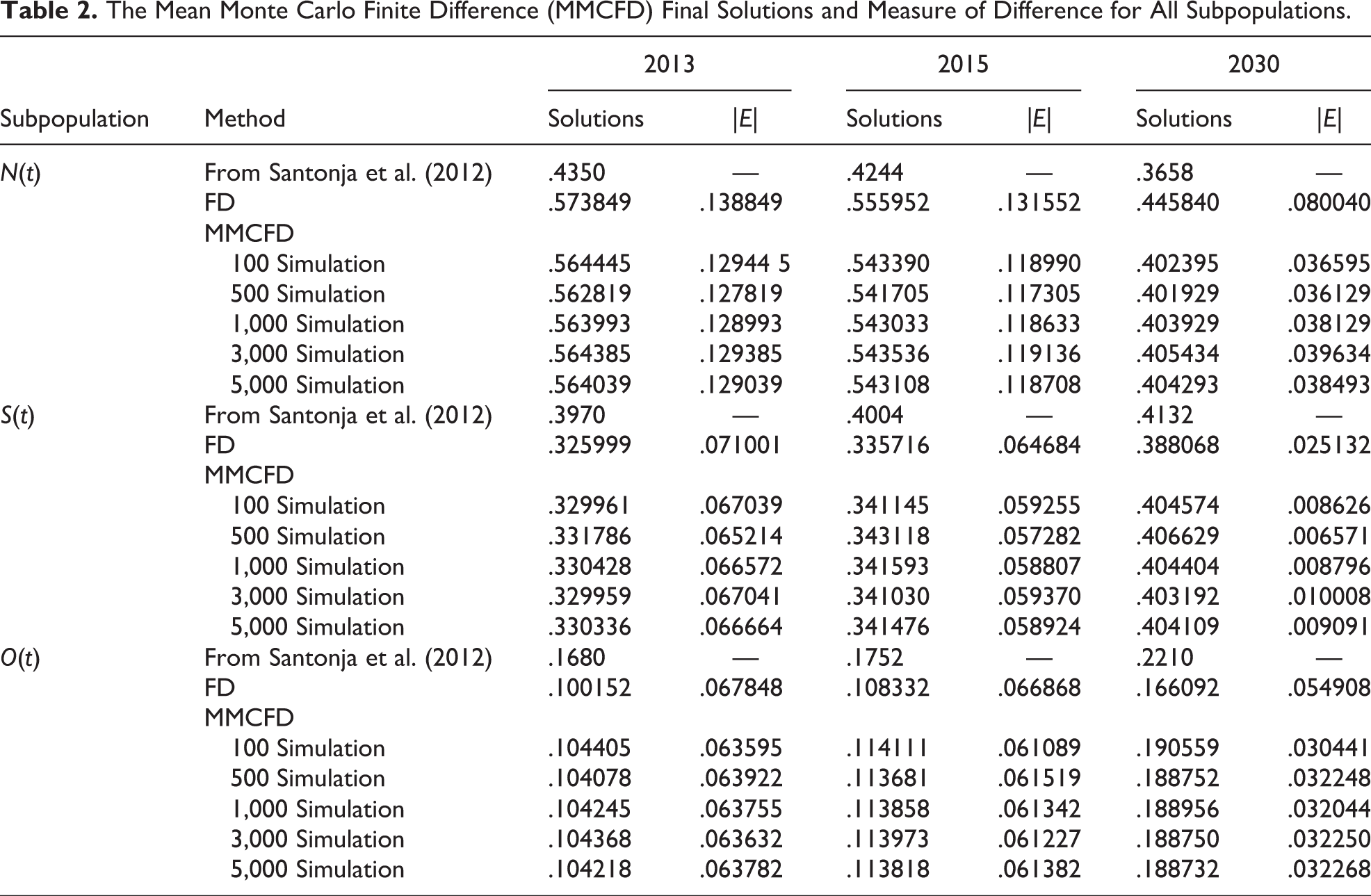
All model parameters (Santonja et al. 2012) are simulated by MC method prior to numerical solutions of the system (7) to (9) by using FD method in MMCFD approach corresponding to specific time interval (Table 2). This process is repeated for 100; 500; 1,000; 3,000; and 5,000 times. As a result, the system has 100 to 5,000 final solutions that are used to calculate their mean. The MMCFD solutions represent the system solution. These mean values correspond to the mean of the last iteration of MMCFD solutions in each repeated simulation cum the mean of the last component of final solutions vector (the end values in the ordered random sample for N(t), S(t), and O(t)) are listed in Table 2. The flow chart of MMCFD procedure is further presented in Figure 1.
The Mean Monte Carlo Finite Difference (MMCFD) Final Solutions and Measure of Difference for All Subpopulations.
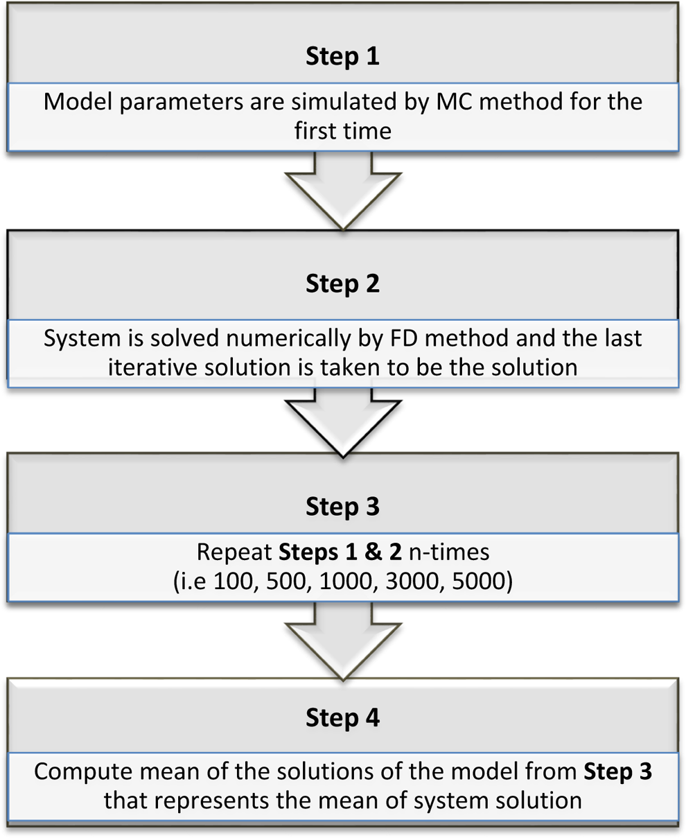
Flow chart of mean Monte Carlo finite difference method.
We compute the time t as a unit in week by using Wolfram Alpha program, where the number of weeks from the beginning of 2001 to the end of 2013 is calculated as 678 weeks, from the beginning of 2001 to the end of 2015 is 782 weeks, and from the beginning of 2001 to the end of 2030 is 1,565 weeks. The number of weeks in each interval is the same number of iterations. Random predictions in 2013 and over the next few years in 2015 and 2030 can be performed by assuming all model parameters to have uniform probability distributions on given intervals (Santonja et al. 2012) since these parameters are random variables. In this case, the outcome results are called as “numerical-simulated solutions” by means of MMCFD method. Since we have previous results for this model that are estimated by a statistical method with estimated parameters (Santonja et al. 2012), comparison between the present MMCFD final solutions with the predicted results (Santonja et al. 2012) is possible. The numerical-simulated solutions of MMCFD are appeared as follows:
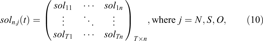
such that each variable N(t), S(t), and O(t) is presented in the above matrix. Then, the solution of the system is:

when T is the maximum number of iterations as well as the number of weeks in each considered intervals (678 weeks in 2013, 782 weeks in 2015, and 1,565 weeks in 2030), and n is the number of random sample space as well as the number of simulation.
The solutions for each variable N(t), S(t), and O(t) in the model using n simulations (taking from the last iteration of equation 11) are represented as the following vector:

Therefore, the solution of the model is:

Hence, the mean of the solutions for each system variable μsol,j is displayed as:

where the MMCFD solutions of the system, μsol, is:

All MMCFD computations are done in MATLAB 13 environment. Some graphical results (for 5,000 simulations) are sketched using MagicPlot (Version 2.7.2) software, while the box plots are drawn by using S-plus 8.1 software.
Statistical Indicators
This study considers certain statistical indicators such as measure of difference |E|, standard deviation of MC (σn), and percentile of distribution in order to compare between MMCFD results and the predicted results (Santonja et al. 2012). For this purpose, we define a measure of difference |E|:

where xsol is a numerical value (the last iteration value of FD or the MMCFD solutions, μsol,j, as in equation 14) and xp is a predicted value from Santonja et al. (2012). Standard deviation σ is calculated as a special measuring of error for the MMCFD method. The expression
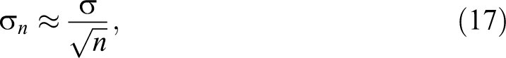
where n represents the number of simulations in the present computation as well as the sample size of the model random variables. Since value of the standard deviation σ of the population is not given, the variance of σn defined as:

is used in the current article with

and

such that j = N, S, O, where soln,j(T) is mentioned in equation (13). In general, the best result is obtained when the standard deviation of the means σn is the smallest (Jacoboni and Lugli 1989).
Another statistical indicator to describe data (solution) is prediction interval. Prediction interval is an interval contains upper and lower bounds for predicted values of the distribution for each subpopulation of the model. It can be obtained by using the pth percentile to give upper and lower limits. A percentile is a value inside a distribution that can divide ordered predicted values into two or more parts by drawing lines between these values. These predicted values belong to the vector distribution of random variable N(t), S(t), and O(t). As a consequence, the pth percentile of the predicted values is inside a population. This percentile value is equal to or less than the number one required to calculate it, when 0 < p < 100. Suppose that n is the total number of predicted values in a distribution (random sample size). The index becomes [(n) × (p ÷ 100)] and represents the place for the pth percentile value within the population distribution. All the predicted values are arranged from the smallest time value (in a week) until the largest time value in the distribution. For example, 0.581503 is the upper limit (95th percentile of N(t) at the end of 2015 for 5,000 simulations) of predicted values inside the population. It means 95 percent of predicted values for the population are equal to or less than 0.581503. The lower limit of this predicted interval is the 5th percentile. The median here is the 50th percentile of the predicted values. In other words, the 50th percentile is a data that split the entire data distribution into two pieces, such that 50 percent of the values lie in one piece and the other values lie in the second piece (Knowelden 1952). Here, we have chosen the 5th and 95th percentile to get a 90 percent prediction interval for our numerical-simulated solutions as an alternative to the 90 percent prediction interval of statistical predictions given by Santonja et al. (2012). Although the 5th and 95th percentiles are selected in the present work, we can also use other percentiles depending on the size of the prediction interval.
Results and Discussion
In this section, the MMCFD solutions are presented for the systems (1) to (3). Since random variables are included as parameters in this model, random variables sampling can be estimated by MMCFD method through MC simulation. Good inference is obtained when all MMCFD solutions are proved to be closer to statistical results (Santonja et al. 2012) than the FD numerical results with difference recurrence of simulations (100; 500; 1,000; 3,000; and 5,000 simulations) in 2013, 2015, and 2030 (Table 2). Since different approaches (numerical and statistical) are employed and due to source of errors, the MMCFD numerical-simulated solutions of the systems (1) to (3) are expected to have a percentage of difference with statistical and FD results spatially at the end of 2013, 2015, and 2030 for the subpopulations N(t), S(t), and O(t) as clearly supported by Tables 2 and 3 and Figures 2 to 4, respectively.
Absolute Growth Rates and Yearly Average Growth Rates of the Subpopulations.

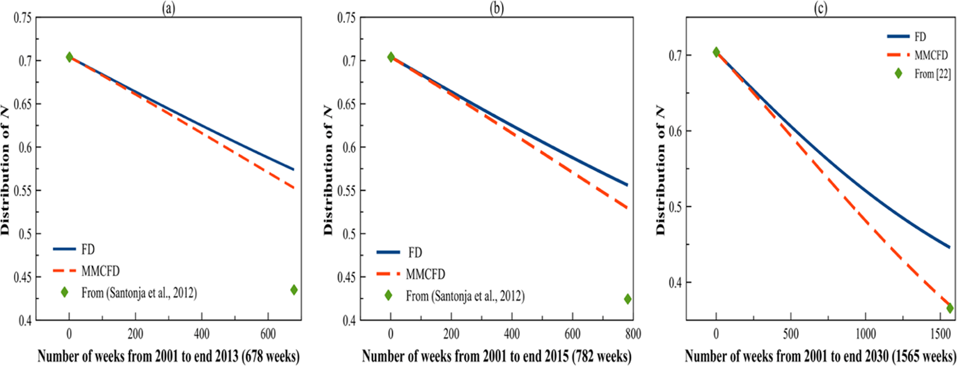
N(t) solutions by using finite difference and mean Monte Carlo finite difference—5,000 simulations from 2001 until the end of (a) 2013, (b) 2015, and (c) 2030.

S(t) solutions by using finite difference and mean Monte Carlo finite difference—5,000 simulations from 2001 until the end of (a) 2013, (b) 2015, and (c) 2030.

O(t) solutions by using finite difference and mean Monte Carlo finite difference—5,000 simulations from 2001 until the end of (a) 2013, (b) 2015, and (c) 2030.
In Table 2, solutions of N(t), S(t), and O(t) are tabulated in comparison with results from Santonja et al. (2012), FD method, and MMCFD method. The corresponding measure of differences between FD and MMCFD methods with respect to statistical predictions (Santonja et al. 2012) are also listed. In general, normal weight subpopulation, N(t), of the Valencia community is expected to reduce as the year increases from 2000 (see Table 1; N0 = 0.704, S0 = 0.250, O0 = 0.046) to 2030, while the subpopulations of overweight S(t) and obese O(t) are growing over the same period. It is observed that the measure of difference of the MMCFD solutions consistently smaller than the measure of difference of the FD method in all years of 2013, 2015, and 2030 under various repeated simulations (100; 500; 1,000; 3,000; and 5,000 simulations). Although the current results depend on 5,000 simulations, different numbers of repeated simulations are tested in Table 2 to find the best number of simulation that produces the closest results to the predicted values (Santonja et al. 2012). In general, the statistical behavior is random with MMCFD method, and it is noted that MMCFD results are extremely convergent with regard to different number of simulations. It is observed that the MMCFD solutions for both normal weight and overweight subpopulations is the most convergent to the predicted values (Santonja et al. 2012) in 500 simulations in all years of 2013, 2015, and 2030. However, the MMCFD results of obese subpopulation in these years are the closest to the statistical values (Santonja et al. 2012) by using only 100 simulations.
On the other hand, the absolute growth rate percentage at the end of 2013, 2015, and 2030 as well as the absolute yearly average growth rate percentage as compared to the initial conditions of each subpopulation in the last week of 2000 (Santonja et al. 2012) are presented in Table 3. It is found that the normal weight N(t) and overweight S(t) subpopulations are decreasing at average rates of 1.6 percent and 2.2 percent per year by statistical prediction (Rohaninejad and Zarghami 2012), at 1.2 percent and 1.8 percent by FD method, and at 1.4 percent and 2.1 percent by MMCFD method, respectively, from the last week of 2000 until the end of 2030. Oppositely, the growth rate of obese subpopulation O(t) is increasing over the 30 years. The average yearly increasing rate for the obese subpopulation is estimated at 12.7 percent, 8.7 percent, and 10.3 percent from Santonja et al. (2012), FD, and MMCFD solutions, respectively. The statistical predictions (Santonja et al. 2012) produce the highest growth rates for all subpopulations and years, the FD method gives the minimum rates, while the MMCFD method provides the intermediate rates between the two different approaches of statistical and numerical methods.
According to Figure 2, normal weight curves for both FD and MMCFD methods are gradually declining. The decrement in N(t) is slightly higher in 2015 than in 2013. It is also noted that the normal weight subpopulations continue to fall until it approaches the predicted value (Santonja et al. 2012) at the end of 2030. This convinces the expectation that N(t) will decrease in future. In general, the normal weight curves for MMCFD are decreasing significantly than the normal weight curves of FD from 2001 to 2030. It is clear that MMCFD curves of normal weight subpopulation converge to the predicted values of Santonja et al. (2012) faster than the FD curves for all 30 years especially at the end of 2030.
Based on Figures 3 and 4, the overweight and obese curves are rising progressively in 2013. Also, the progress is more evidenced in 2015 as compared to 2013. Moreover, S(t) and O(t) are approaching the predicted values (Santonja et al. 2012) closely at the end of 2030. In other words, S(t) and O(t) are expected to increase with MMCFD overweight, and obese curves are consistently higher and closer to the predicted solutions (Santonja et al. 2012) than the FD curves in all years. Even though all curves of normal weight, overweight, and obese starting at the same initial points in the beginning of 2001, however only MMCFD solutions for all N(t), S(t), and O(t) are closer to the given predicted points (Santonja et al. 2012) at the end of 2013, 2015, and 2030 as compared to the FD solutions. It can be concluded that random error from simulation causes difference between FD and MMCFD results and the error increases with more iterations in the future as showed in Figures 2 to 4.
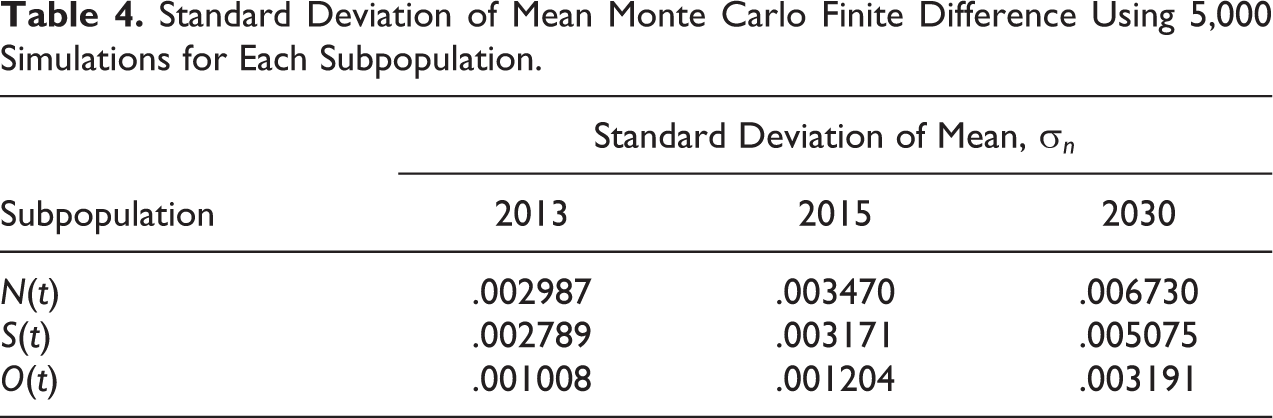
From Table 4, the standard deviation of mean, σn, in equations (17) to (20) of MMCFD for all subpopulations until 2030 is sufficiently small. Therefore, this indicator signifies an acceptable error (Jacoboni and Lugli 1989) for present work. From 2001 to 2030 at 5,000 simulations, standard deviation of error for normal weight subpopulation is not more than 0.006730, while the standard deviation of error for overweight individual drops to 0.005075. At the same time, the standard deviation of error for obese falls to 0.003191. The important point to be addressed here is the MMCFD standard deviation of mean, σn, has a very low percentage of error as evidenced in Table 4. Finally, σn increases with years as a result of statistical simulation errors.
Standard Deviation of Mean Monte Carlo Finite Difference Using 5,000 Simulations for Each Subpopulation.
The predicted intervals of MMCFD solutions are approaching the range of intervals by Santonja et al. (2012) with a percentage of error (see Table 4 in Santonja et al. 2012 and Table 5). In general, many factors can cause errors in the present study. Firstly, modeling error might happen in the systems (1) to (3) as given in Santonja et al. (2012), where this error comes from prediction and actual data. Secondly, the sampling and rounding errors come from simulation method to estimate model parameters that are later being transported to predictions. The third source of the error is due to different simulation techniques to estimate model parameters. In the present work, the parameters are simulated by using the classical MC process, while in Santonja et al. (2012), the parameters are simulated 5,000 times by using LHS technique that is another type of MC sampling. Finally, the error comes from the type of distribution (uniform distribution) for parameters and solutions of the model (Santonja et al. 2012). The numerical method is subjected to two common numerical errors, the round off error which losing of precision due to computer rounding of decimal quantities and data propagation error. Therefore, the error is not restricted and extends in all interval areas of the distribution.
Prediction Intervals [5th Percentile, 95th Percentile] of Mean Monte Carlo Finite Difference Solutions for N(t), S(t), O(t) Using 5,000 Simulations at the End of 2013, 2015, and 2030.
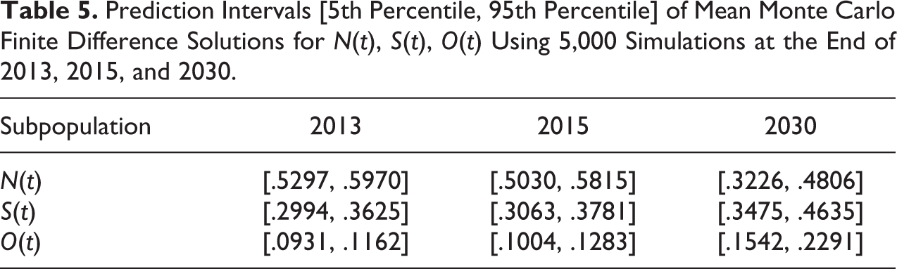
Because of random sampling and rounding errors in the particular model, the solutions can be presented by predicted interval of N(t), S(t), and O(t). The predicted interval consists of percentiles of final solutions for each variable N(t), S(t), and O(t) running at 5,000 evaluations, empirically at 5th and 95th percentiles. These percentiles are used to account 90 percent prediction interval that implies 90 percent of the predicted values inside this interval. Consider predicted intervals of distributions for N(t), S(t), and O(t) contain a lower limit (5th percentile) and an upper limit (95th percentile). Based on MMCFD solutions with 5,000 simulations, the predicted values inside the population is variously distributed for different years (see Table 5 and Figures 5 –7).

The 5th, 50th, and 95th percentiles for mean Monte Carlo finite difference solutions of N(t) with 5,000 simulations from 2001 until the end of (a) 2013, (b) 2015, and (c) 2030.
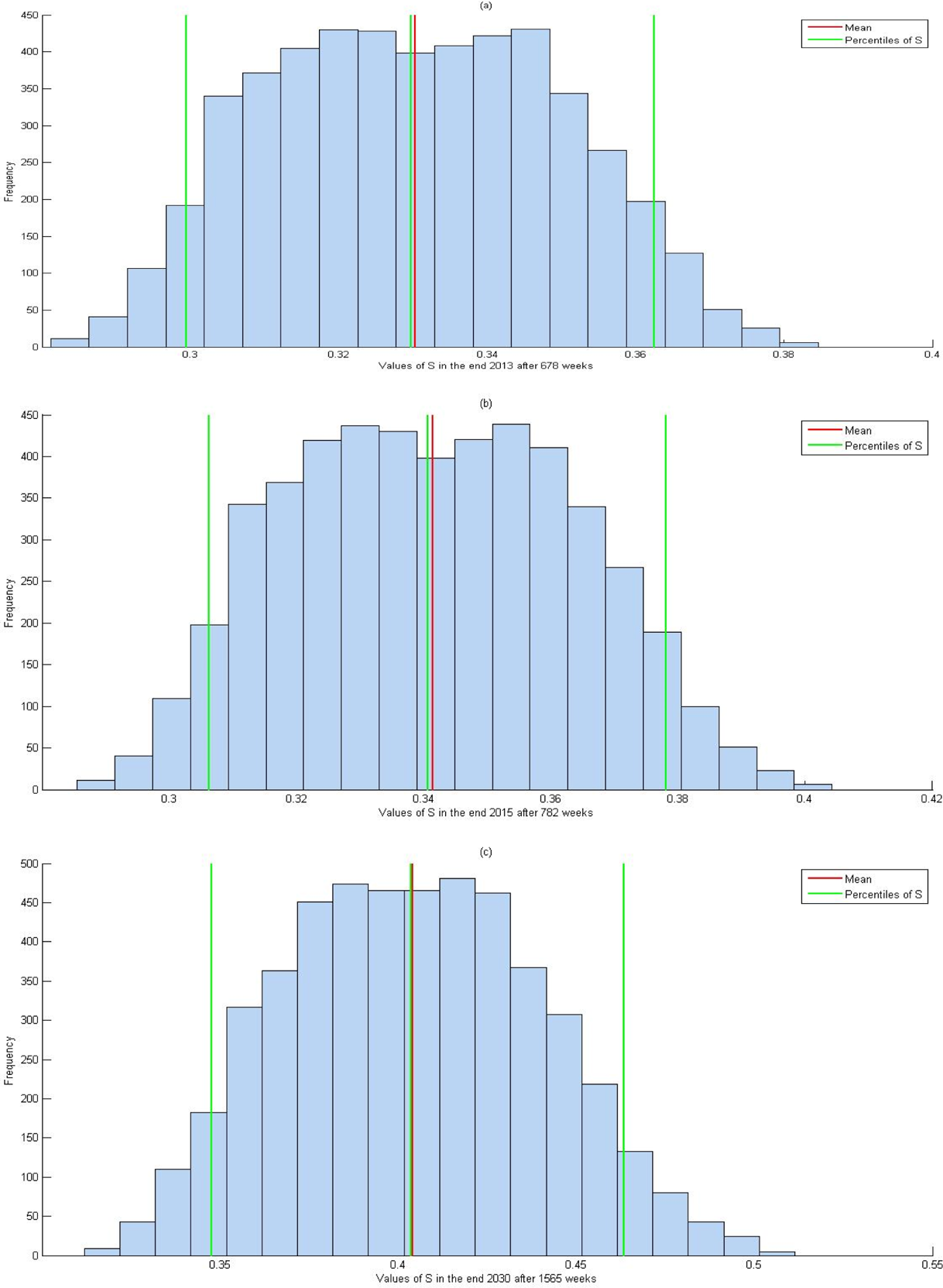
The 5th, 50th, and 95th percentiles for mean Monte Carlo finite difference solutions of S(t) with 5,000 simulations from 2001 until the end of (a) 2013, (b) 2015, and (c) 2030.
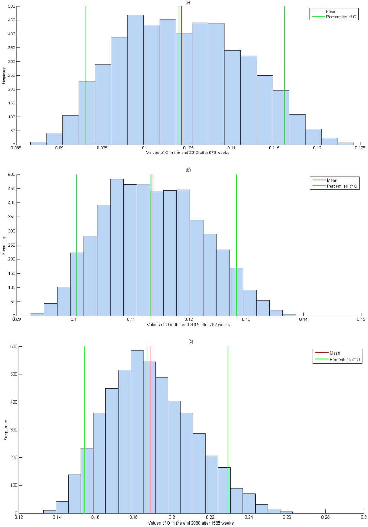
The 5th, 50th, and 95th percentiles for mean Monte Carlo finite difference solutions of O(t) with 5,000 simulations from 2001 until the end of (a) 2013, (b) 2015, (c) 2030.
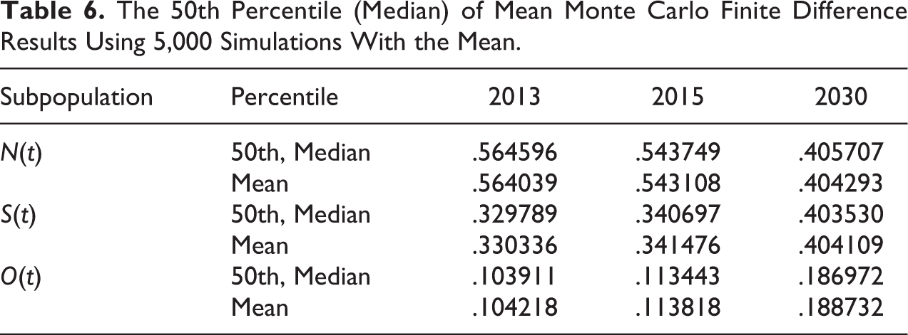
Comparing between the present MMCFD results and the statistical predicted intervals, Santonja et al. (2012) presented 90 percent prediction intervals for N(t), S(t), and O(t) as listed in Table 4 (Santonja et al. 2012:37), which are taken from the empirical 5th and 95th percentiles. The current MMCFD-predicted interval consists of percentiles of N(t), S(t), and O(t) empirically at 5th and 95th percentiles too. Both predicted intervals of solutions to this model are obtained by using 5,000 simulations of model parameters. It is clear that all MMCFD solutions in Tables 2 and 6 with 5,000 simulations are inside the predicted intervals of percentile as presented in Table 5. In addition, the 50th percentile as the median for MMCFD solution distributions is close to the mean of these solutions as shown in all Figures 5 to 7 from 2001 to the end of 2013, 2015, and 2030, respectively.
The 50th Percentile (Median) of Mean Monte Carlo Finite Difference Results Using 5,000 Simulations With the Mean.
Box plots analyzing the results of N(t), S(t), and O(t) from 2001 to 2030 are provided graphically in Figure 8. They show the central point (median), the extreme values (maximum and minimum values), and the outliers which are the points outside the boundaries. The box plots present the pattern of the MMCFD solutions of N(t), S(t), and O(t) throughout the 30 years. Using 5,000 simulations, the box plot of N(t) lays above in 2013 with one outlier point at bottom, declines significantly from 2015-2030. It means the subpopulation values of N(t) take smaller values in the end of 2030 as compared to 2013 and 2015 (see median in Table 6). Inversely, the box plots of S(t) and O(t) are located at the bottom in 2013, then they rise slightly in 2015 with major hikes in 2030. There is only one outlier value above the box for S(t) in 2030, but more outliers are at the top part of the box for O(t) in 2030. It means the subpopulation values of S(t) and O(t) have greater values at the end of 2030 than in 2013 and 2015 (see median in Table 6). The statistical behaviors shown in Figures 2 to 4 and in Figure 8 confirmed that N(t) will decrease while S(t) and O(t) will increase in the future.

Box plots along 30 years (2001–2030) of mean Monte Carlo finite difference solutions With 5,000 simulations for (a) N(t), (b) S(t), (c) O(t).
Conclusion
In this study, the MMCFD method is proposed for the first time to solve an epidemiology model explicating the effects of public health campaign on body weight loss in Spain. The MMCFD method is suggested to generate new numerical-simulated solutions for this model, so that random variables sampling can be estimated by MC method. It is found that the MMCFD method produced numerical-simulated solutions of the model with better approximation toward previous statistical predictions as compared to the FD method in all time intervals considered. Through this work, it is shown that the MMCFD method is beneficial to generate random coefficient sampling for the nonlinear epidemic system. Besides, the MMCFD method is also promising to create agreement and estimation balance between a statistical method and a classical numerical method.
Footnotes
Acknowledgments
The authors thank the reviewers for their valuable suggestions and comments for the improvement of this article.
Declaration of Conflicting Interests
The author(s) declared no potential conflicts of interest with respect to the research, authorship, and/or publication of this article.
Funding
The author(s) received no financial support for the research, authorship, and/or publication of this article.