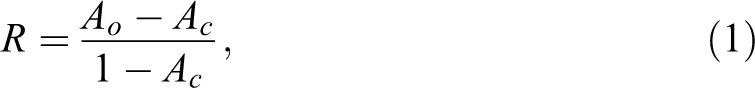
Measuring Social Class with Changing Occupational Classifications: Reliability,Competing Measurement Strategies,and the 1970

Abstract

Periodic changes in occupational classifications make it difficult to obtain consistent measures of social class over time, potentially jeopardizing research on class-based trends. The severity of this problem depends, in part, on the measurement strategies used to address those changes. The authors propose that when a sample has been coded partly with one occupational classification and partly with another, Krippendorff’s index α be used to identify the best strategy for measuring class consistently across the two classifications and to assess the reliability of the class measure employed in the final analyses. This index can be computed regardless of the metric of the class variable; it can be used to compare measures based on different class schemes or that use different metrics; and statistical inference is straightforward, even with a complex sampling design. The authors put the index to work in conducting a case study of the effects of the switch from the 1970 to the 1980 U.S. Census Bureau Classification of Occupations on the reliability of Erikson–Goldthorpe–Portocarero class measures. Their findings indicate that measurement strategies that seem a priori equally reasonable vary substantially in terms of their reliability, and that the bulk of this variation is accounted for by the extent to which the strategies rely on subjective judgments about the relationships between occupational and class classifications. Most importantly, as long as the best-performing measurement strategies are used, the switch in occupational classifications appears to be substantially less consequential than has been previously argued. A computer program made available as a companion to the paper makes estimation of Krippendorff’s α, and statistical inference, very simple endeavors for nominal class variables.

Keywords

social class measurement reliability Krippendorff’s α Erikson–Goldthorpe–Portocarero class scheme occupational classification

Introduction

The study of long-term trends related to social classes—trends regarding a country’s class structure, differences in political attitudes across classes, and intergenerational social mobility, to mention three prominent examples—requires that social class be measured consistently over time.¹ But consistent measures of social class can be hard to obtain. Class measures are typically derived from occupation variables (and sometimes other variables as well, such as self-employment status), and the classifications used to code occupations change periodically as they are improved conceptually and updated to account for changes in the occupational structure. When a data set is coded partly with one occupational classification and partly with another, it can greatly affect social scientists’ ability to study class trends. The severity of the problem depends, in part, on the nature and scope of the changes in the occupational classifications, but to a very large degree it also depends on the strategies used to deal with these changes.

There are usually multiple measurement strategies that can be used to “bridge” two occupational classifications, and a priori they often seem equally sensible. How do we know whether any given strategy produces a measure of social class reliable enough to study trends? How should we select among the available strategies? For nominal class measures, how can we determine the number of classes (or “granularity”) to use in our analyses, given the potential trade-off between granularity and reliability? Similarly, if a class scheme favored on theoretical grounds is suspected to be less reliable than others that are also acceptable, how can we establish the reliability cost of using the theoretically preferred scheme?

Perhaps surprisingly, methodological tools for addressing these issues are not available, as social scientists have not developed any systematic approach for assessing the reliability performance of different measurement strategies when studying class-based trends across a change in occupational classifications. The main goal of this article is to advance such an approach. We propose that a reliability index extensively used in the field of content analysis, Krippendorff’s α (e.g., Krippendorff 2013:chapter 12), be used to assess the performance of different measurement strategies. Among the key properties of this index are that it accommodates any metric (including nominal, ordinal, interval, and ratio) and that, unlike many other reliability indices, it models “chance agreement” in a way that is both theoretically well-founded and pragmatically fruitful. As long as the researcher has access to a subsample that has been coded using both the new occupational classification and its predecessor—and such double-coded data are often available—it is possible to estimate the index and use it to subject different measurement strategies to systematic empirical evaluation.

We also conduct a case study in which we use the index to examine the effects of the switch from the 1970 to the 1980 Census Bureau Classification of Occupations in the United States. Unlike other changes in occupational classifications in the country, that switch involved a deep conceptual and empirical discontinuity (Vines and Priebe 1989). Researchers have interpreted this discontinuity as making very difficult, if not simply precluding, consistent measurement of social class across the 1970–1980 divide, and this has greatly hindered the study of class-related trends. In the case of intergenerational mobility, for instance, Beller (2009) maintained that “[t]rends in social class fluidity after the mid-1980s are unclear, in part because changes to the census coding of occupations in the 1980s made it impossible to directly compare new survey data with older data” (p. 509; references omitted). It has been further argued that the problem is particularly serious when working with the widely used Erikson–Goldthorpe–Portocarero (EGP) class scheme (e.g., Erikson and Goldthorpe 1992). For instance, in a study of social class differences in the earnings of black and white men, Morgan and McKerrow (2004) asserted that it is not possible to reconcile the 1970 and 1980 classifications without introducing substantial distortions into the data, especially when implementing the EGP class scheme (supp. app.), and for this reason they focused on the period starting in 1983.² The reported difficulties have not completely precluded the study of U.S. class-based trends across the 1970–1980 divide using the EGP scheme (see Hout 2005; Mitnik, Cumberworth, and Grusky 2016; Pfeffer and Hertel 2015; Weeden et al. 2007). However, none of these studies provided any systematic assessment of the reliability of the class measures they used, either in absolute terms or compared to other possible measures.³

In our case study, we examine whether the obstacles to obtaining a reliable EGP measure of social class across the 1970–1980 classification divide are as fundamental as has been claimed. Using double-coded data from the General Social Survey (GSS; see Smith et al. 2011), we assess how seven different measurement strategies fare in terms of reliability and in terms of how they perform when used to estimate a common model of intergenerational class mobility. Our results indicate that (a) the strategies, which seem equally reasonable a priori, vary substantially in terms of their reliability, (b) this variation in reliability is largely accounted for by the extent to which the strategies rely on researchers’ subjective judgments about the relationships between occupational and class classifications, and (c) as long as the best-performing strategies are used, the problems generated by the 1970–1980 classification divide appear to be substantially less consequential than has been argued in the literature.

Although in our case study we use the GSS—taking advantage of the double-coded data this survey has long included—and focus on one particular change in occupational classifications and one class scheme, our results are broadly relevant for research on class-based trends. First, they are directly relevant for research on EGP-based trends in the United States using other data sets partly coded with the 1970 occupational classification and partly coded with the 1980 occupational classification.⁴ Second, they suggest more general lessons for research on class-based trends in the United States using other class schemes, and for similar research dealing with changes in occupational classifications in other national or temporal contexts.

This article is organized as follows. In the next section, we introduce Krippendorff’s α and explain its conceptual advantages over several other widely used reliability indices. The form of the index we present in this section is very general and makes its conceptual foundations transparent but is not convenient for computational purposes. In the following section, we therefore introduce a second expression—for nominal class variables only—that makes it much easier to compute point estimates and conduct statistical inference. The fourth section is devoted to our case study. The last section presents our main conclusions.

Reliability and Social-Class Measurement Strategies

In the context of measurement theory, reliability is the extent to which a measurement procedure provides the same results under repeated measurement of the same units; a procedure is considered reliable as long as it tends to produce consistent results across measurements. In turn, data are reliable as long as they have been produced using a reliable procedure. Reliability is distinguished from validity, which pertains to the extent to which a measuring procedure measures what it purports to measure. Reliability is usually interpreted as a precondition for validity (e.g., Carmines and Zeller 1979).

When measuring social class across a change in occupational classifications, a researcher aims to use a reliable measurement procedure—that is, a procedure that assigns people the same class values regardless of which occupational classification was used to code their occupations. For each of the two occupational classifications, the researcher uses a set of rules to assign class values to occupations.⁵ We refer to these sets of rules as “occupation-to-class mappings” or just “mappings.” Together, the two mappings constitute a measurement strategy.⁶ We can therefore say that the researcher’s goal is to use a reliable measurement strategy.

If part of the sample (i.e., a subsample) has been double-coded using the two occupational classifications, the extent to which any strategy approaches the ideal of full reliability can be empirically assessed. To conduct such an assessment, the researcher would assign everyone in the double-coded sample two class values, using the two mappings in the measurement strategy. Loosely speaking, the greater the agreement between the class assignments across mappings, the more reliable the measurement strategy is.

In order to make this loose idea operational, the researcher needs a reliability index to quantify the degree of agreement, to determine whether a particular strategy reaches the minimum level of reliability deemed acceptable, and to compare the reliability of different strategies. Below, we critically examine a set of indices that have been used extensively in various fields to assess reliability. Then, we introduce Krippendorff’s α, which is the index that we favor.

Critical Assessment of Widely Used Reliability Indices

An index that has often been used to assess the reliability of interval variables is the correlation coefficient. This is a very flawed approach, as it confuses predictability with reliability. In our context, the correlation coefficient would provide information about how well the class values produced by one occupation-to-class mapping linearly predict the values produced by the other. But one mapping’s values can perfectly predict the other’s even in cases where the two sets of values are completely different.

For nominal variables, the reliability index that perhaps seems most intuitive is the simple percent agreement—in our case, the percent agreement between two occupation-to-class mappings. For example, a measurement strategy where 80 percent of people are mapped into the same classes by both mappings seems clearly more reliable than a strategy where only 50 percent are mapped into the same classes. But intuitive as it may seem, percent agreement is a very unsound measure of reliability as well. It ignores that some level of agreement would occur even if class categories were assigned randomly (e.g., Mielke and Berry 2001:134). Therefore, it badly overstates the reliability of the data. Equally concerning, given that the agreement expected by chance, or “chance agreement,” is a function of the number of class categories, using the percent agreement as a reliability index makes meaningless any comparisons between class measures with different numbers of categories.

Several measures of reliability for nominal variables have been proposed that do take into account that agreement may occur by chance and therefore include a correction for chance agreement. They all have the following form (Zwick 1988):

R = \frac{A_{o} - A_{c}}{1 - A_{c}},

where R is a reliability measure, $A_{c}$ is the chance proportion of agreements as this is defined under R, and $A_{o}$ denotes the observed proportion of agreements (i.e., the proportion of observations in which the mappings agree in their social class assignments).

Figure 1 shows the basic structure of a cross tabulation of data used to assess the reliability of a measurement strategy for a nominal class variable. The figure shows the same K class categories in rows and columns. The class measure produced by mapping the first occupational classification into the class categories (mapping 1) is in rows, and the measure produced by mapping the second occupational classification into the class categories (mapping 2) is in columns. In the figure, $p_{i j}$ denotes the proportion of people assigned to class i by mapping 1 and to class j by mapping 2, while $p_{i .}$ is the proportion of people assigned to class i by mapping 1 and $p_{. j}$ is the proportion of people assigned to class j by mapping 2. In all reliability measures for nominal variables, $A_{0} = \sum_{k = 1}^{K} p_{k k},$ that is, the observed agreement is simply the sum of the quantities in the main diagonal. The reliability measures differ, however, in how they define $A_{c} .$

Figure 1.

Cross tabulation of nominal class measures produced by a measurement strategy’s mappings.

Bennett, Alpert, and Goldstein (1954) first proposed the reliability index S, which has since been reintroduced under many other names (see Zwick 1988). Under this index, chance is modeled as the random assignment of classes to people, assuming a uniform probability over class categories. The probability of any ordered pair of values is then $\frac{1}{K^{2}}$ , so the expected proportion of agreements is $A_{c} = K \frac{1}{K^{2}} = \frac{1}{K} .$ The index equals one when there is perfect agreement and zero when agreement is as expected by chance. Its main shortcomings are that (a) the value of S can be large even if the two mappings produce very different marginal distributions of the class variable, when this should result in low reliability values, (b) if the mappings assign classes randomly, the values of S will be larger the more disagreement there is about marginal distributions (for these two issues, see Hsu and Field 2003), and (c) for a given value of $A_{o},$ the value of S increases as K (the number of classes) increases, even if no one is assigned the added classes (Scott 1955).

Cohen’s (1960) κ stipulates $A_{c} = \sum_{k = 1}^{K} p_{k .} p_{. k}$ . Thus, chance agreement here is the agreement that can be expected if classes are randomly and independently assigned to people within each mapping, with probabilities equal to the mapping-specific observed relative frequencies of the class categories. Although used widely in epidemiology and other fields, Cohen’s κ is also seriously flawed. The main problem is that, for any given level of agreement (any value of $A_{o}$ ) κ penalizes agreements in marginal distributions across mappings, that is, κ is lower the more agreement there is between those distributions. The reason for this undesirable result is that the index takes the marginal distributions as priors; thus, two mappings that produce similar marginal distributions must achieve a much higher agreement rate to obtain a given value of κ than mappings that produce radically different marginal distributions (Brennan and Prediger 1981:692; see also Warrens 2012 and the references therein). Or, as Krippendorff (2004:420-21) has shown, the better disagreement can be predicted, the higher the value of κ, which conflates predictability with agreement.

Scott’s π defines $A_{c} = \sum_{k = 1}^{K} {(\frac{p_{k .} + p_{. k}}{2})}^{2}$ , so chance agreement here is the agreement that can be expected if classes are assigned to people with probabilities equal to the best available estimates of their true prevalence in the population (Scott 1955:324), that is, their average prevalence across mappings. Unlike Cohen’s κ, Scott’s π does not confuse predictability with agreement (Krippendorff 2004:420-21). Although a sound reliability index, π has a “scope limitation” that it shares with S and κ: None of these indices can be used to establish the reliability of data based on metrics other than the nominal metric (e.g., ordinal, interval, and ratio). As we indicate below, π is a particular case of our preferred and most general reliability index, Krippendorff’s α.

Before introducing this index, a few words regarding Cronbach’s (1951) α, which is presented as a reliability measure and has often been used in sociology, seem in order. In our context, the relevant notion of reliability is reliability-as-replicability—the reproducibility of results across functionally equivalent measurement instruments. Cronbach’s α, however, measures internal consistency (e.g., of the items in a psychometric test). Whatever its merits and limitations in this regard (see Sijtsma 2009 for a detailed analysis), it belongs to the family of correlation coefficients, and it shares their shortcomings if used as a measure of reliability.

Krippendorff’s α

Krippendorff’s α is defined (e.g., Krippendorff 2013:chapter 12) as:

α = 1 - \frac{D_{o}}{D_{e}},

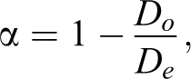
where $D_{o}$ and $D_{e}$ are the measures of observed and expected disagreement, respectively. The index ranges from 1 when there is no disagreement (i.e., when there is perfect agreement) to 0 when observed and expected disagreement are the same.⁷

In our case, which involves two occupation-to-class mappings per measurement strategy, observed disagreement can be expressed as:

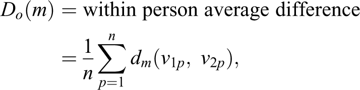
D_{o} (m) = within person average difference = \frac{1}{n} \sum_{p = 1}^{n} d_{m} (v_{1 p}, v_{2 p}),

where n is the number of people in the reliability sample (i.e., the double-coded sample); $v_{q p}$ is the class assigned to person p by mapping q, $q = 1, 2;$ and $d_{m}$ is the difference function under metric m, where m is nominal, ordinal, interval, or ratio. Expressions for these difference functions are provided below.⁸

The disagreement expected by chance is here the expected disagreement when the class values assigned to people are statistically independent from people’s actual values, and the marginal distribution of the values is the one implied by the actual assignments pooled across mappings. More precisely, assume a stochastic process in which the pair of class values found for each person (i.e., one value from each mapping) is the result of randomly selecting, with equal probability, one of the $2 n (2 n - 1)$ 2-permutations (or partial permutations of size 2) of the set of $2 n$ values actually assigned by the mappings to the n people in the reliability sample. A physical implementation of the random assignment just described could be achieved as follows. For each unit in the reliability sample: (a) flip a coin to define which mapping “draws” first, (b) the selected mapping randomly draws one value from the 2n available values, and (c) the other mapping randomly draws one value from the remaining (2n − 1) values. Under this model of chance, expected disagreement is the average difference across all possible $2 n (2 n - 1)$ 2-permutations, which can be expressed as:⁹

D_{e} (m) = within data average difference = \frac{1}{2 n (2 n - 1)} \sum_{i = 1, j = 1}^{n} \sum_{k = 1, l = 1}^{2} d_{m} (v_{k j}, v_{l i}) .

The index can then be written as:

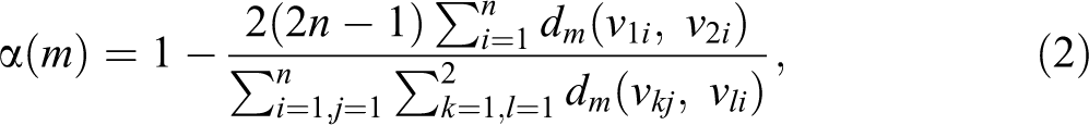
α (m) = 1 - \frac{2 (2 n - 1) \sum_{i = 1}^{n} d_{m} (v_{1 i}, v_{2 i})}{\sum_{i = 1, j = 1}^{n} \sum_{k = 1, l = 1}^{2} d_{m} (v_{k j}, v_{l i})},

where:

d_{nominal} (c, k) = I (c \neq k),

d_{ordinal} (c, k) = {(\sum_{g = c}^{g = k} F_{g} - \frac{F_{c} + F_{k}}{2})}^{2},

d_{interval} (c, k) = {(c - k)}^{2},

d_{ratio} (c, k) = {(\frac{c - k}{c + k})}^{2},

I is the indicator function (i.e., a function that equals 1 if its argument is true and 0 otherwise), and $F_{j}$ is the total number of observations assigned to category j by the two mappings combined.¹⁰

At least three well-known indices are particular cases of Krippendorff’s α when, as here, only two mappings are included in a measurement strategy (Hayes and Krippendorff 2007; Krippendorff 1970): α approaches Scott’s π when the sample is large and the metric is nominal, and it is equal to Spearman’s rank correlation coefficient and to Pearson’s intraclass correlation coefficient when the metrics are ordinal and interval, respectively. In addition, by making $D_{o} = 1 - A_{0}$ and $D_{e} = 1 - A_{c}$ , it is easy to see that, in the case of the nominal metric, α is also a particular case of Zwick’s (1988) expression (see equation [1]).¹¹

Krippendorff’s α is highly attractive as a reliability measure. It avoids the category mistake of conflating predictability and agreement. It takes into account that agreement may occur by chance, and it assesses deviations from perfect reliability by the proportion of observed to expected disagreement. Its (typical) range of variation has a clear interpretation, with 1 indicating perfect agreement and 0 indicating the same level of agreement as would be expected by chance.¹² By modeling chance agreement as the agreement that would occur if classes were assigned to people independently from their actual classes, it avoids the drawbacks associated with other measures that also take into account that agreement may occur by chance. In particular, Krippendorff’s α punishes dissimilarity (and rewards similarity) between mapping-specific marginal distributions and is fully unaffected by the inclusion or exclusion of unused class categories. Further, α allows fair reliability comparisons between class measures of different granularity and between class measures that operationalize different theoretical approaches. And it can be computed for literally any metric, which has the additional advantage of allowing reliability comparisons even across metrics (e.g., of nominal versus interval social class variables). Lastly, α admits several other useful interpretations (Krippendorff 2013:chapter 12), including that it measures the extent to which the proportion of the undesirable to total disagreements subtracts from perfect agreement, where desirable and undesirable disagreements (in the assignment of class values to people) are those between and within people, respectively, and total disagreement is the sum of these two types of disagreements.

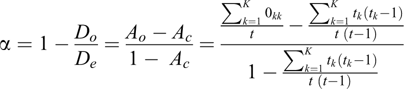
Krippendorff’s α with Nominal Class Variables: Computation and Statistical Inference

The expression for Krippendorff’s α provided by equation (2) is very general but is not convenient for computational purposes. Computationally simpler expressions are available, in particular when class variables have a nominal metric (Krippendorff 2011). As this is the relevant metric for our case study and for much research on class-based trends, in what follows we focus exclusively on the nominal-metric case.

The computationally simpler expression we use is based on a coincidence matrix, which is a square and symmetric values-by-values matrix. This matrix records each pair of class values assigned to the people in the reliability sample twice, with the values in the pair “switching order.” For instance, if person p was assigned the pair of class values $(v_{1 p}, v_{2 p})$ , both this pair and $(v_{2 p}, v_{1 p})$ are included in the matrix.

Figure 2 shows an example of how a coincidence matrix is constructed. In the example, the reliability sample includes six people, and the class scheme comprises three class positions: Manual worker (MW), nonmanual worker (NMW), and professional or manager (PM). The left panel of the figure shows the reliability sample as a standard data set with people as observation units and two variables containing the class values assigned by the two mappings. The right panel shows the coincidence matrix constructed from these data (observe, in particular, that the total number of assigned values, i.e., 12, is the same in both cases). Figure 3 shows the notation we use to refer to the different quantities in a general coincidence matrix. Using this notation, the much-easier-to-compute expression for α with a nominal class variable is:

α = 1 - \frac{D_{o}}{D_{e}} = \frac{A_{o} - A_{c}}{1 - A_{c}} = \frac{\frac{\sum_{k = 1}^{K} 0_{k k}}{t} - \frac{\sum_{k = 1}^{K} t_{k} (t_{k} - 1)}{t (t - 1)}}{1 - \frac{\sum_{k = 1}^{K} t_{k} (t_{k} - 1)}{t (t - 1)}}

= \frac{(t - 1) \sum_{k = 1}^{K} o_{k k} - \sum_{k = 1}^{K} t_{k} (t_{k} - 1)}{t (t - 1) - \sum_{k = 1}^{K} t_{k} (t_{k} - 1)},

Figure 2.

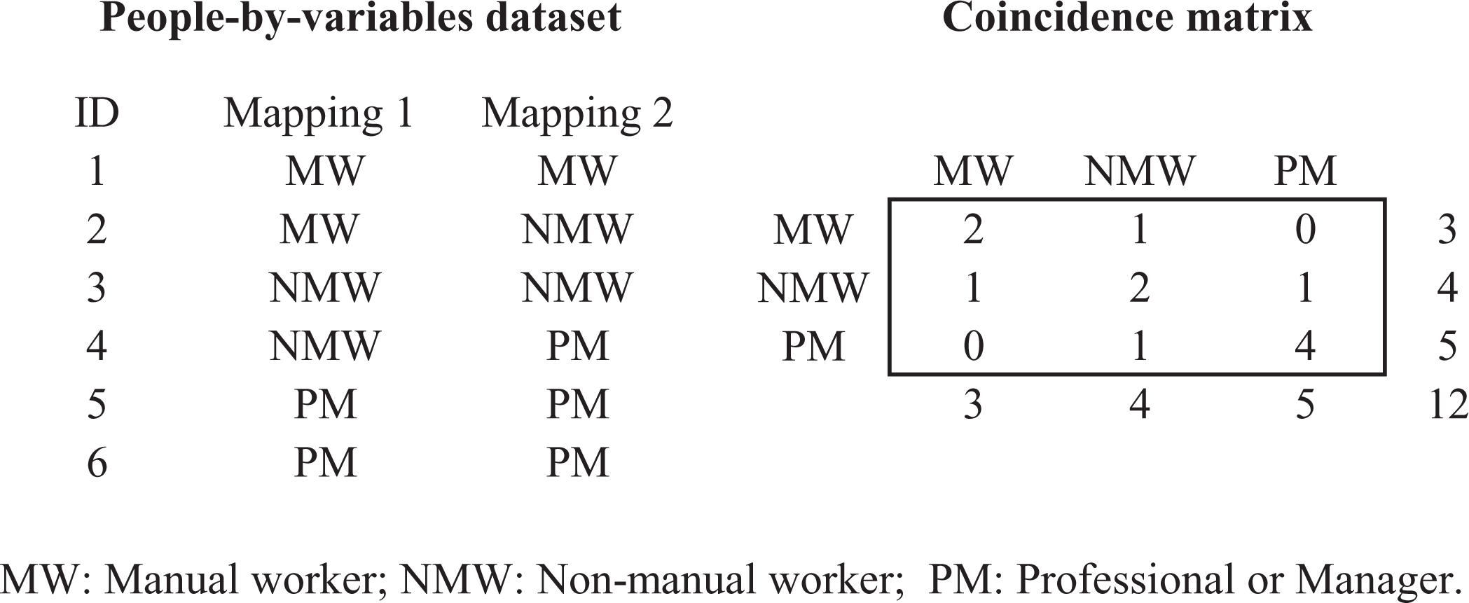
Example of a reliability sample (standard and coincidence-matrix representations).

Figure 3.

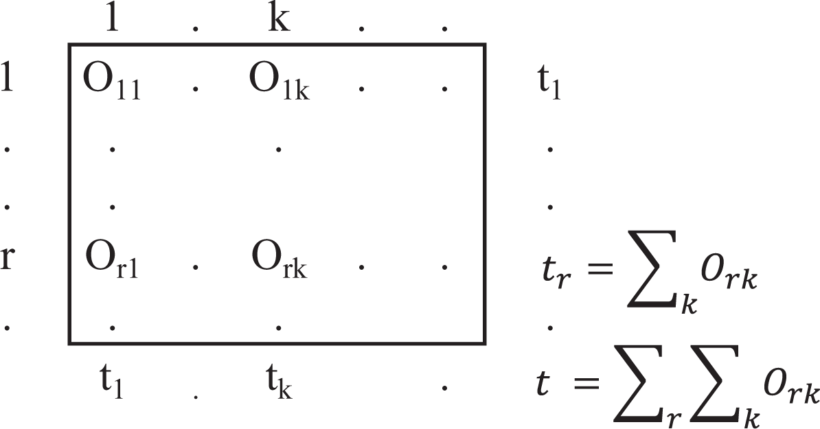
General coincidence matrix.

where $t = \sum_{k = 1}^{K} t_{k}$ is the total number of assigned values (or twice the number of people in the reliability sample), $t_{k}$ is the absolute frequency of class value k in the marginal distribution of class values (or the total number of times the value k was assigned by the mappings), and $o_{k k}$ is the k element in the main diagonal of the coincidence matrix (or twice the number of people both mappings coded as belonging to class k). As should be apparent, in contrast to equation (2), computation of Krippendorff’s α with equation (3) is a very simple exercise once the coincidence matrix has been generated.

In addition to providing the basis for an easy-to-compute expression, working with a coincidence matrix makes it possible to conduct statistical inference without having to resort to resampling approaches and to deal with complex sampling designs easily. To the best of our knowledge, neither of these two advantages has been previously discussed in the literature on Krippendorff’s α.

Let’s assume for now that both the main sample and the reliability sample are simple random samples (SRS)—the main sample an SRS of the population of ultimate interest, and the reliability sample an SRS of the main sample. A value of α computed from a reliability sample is an estimate of the parameter of interest (the population to which that parameter pertains is discussed below) and is therefore subject to sampling variability. But the asymptotic distribution of $\hat{α}$ is unknown, so previous research has proposed basing statistical inference on the nonparametric bootstrap (Hayes and Krippendorff 2007; Krippendorff 2013:chapter 12). This is a highly computer- and time-intensive approach (the recommended number of bootstrap samples is 20,000), and its implementation is somewhat complicated (see Krippendorff [2006] 2016).

The alternative approach we propose here is to use the “delta method” (e.g., Oehlert 1992). This involves computing, first, estimates of $o_{k k}$ and $t_{k}$ for $k = 1, 2, \dots, K$ , which we denote by ${\hat{o}}_{k k}$ and ${\hat{t}}_{k}$ , and of their variance–covariance matrix, which we denote by $\hat{V}$ . With this information in hand, we can use that $\hat{α} = g ({\hat{o}}_{11} \dots {\hat{o}}_{K K}, {\hat{t}}_{1} \dots {\hat{t}}_{K})$ , and therefore $\hat{V a r} (\hat{α}) = \hat{V a r} (g ({\hat{o}}_{11} \dots {\hat{o}}_{K K}, {\hat{t}}_{1} \dots {\hat{t}}_{K}))$ , which allows a standard application of the delta method, and then do statistical inference using standard asymptotic procedures.¹³ Estimates of the elements of the coincidence matrix, and their variance–covariance matrix, can be generated very easily from data in standard form, regardless of the number of class categories.¹⁴

Let’s now assume that while the reliability sample is an SRS of the main sample, the latter is not an SRS of the population of ultimate interest. Rather, the main sample has been drawn using a “complex survey design” (e.g., Heeringa, West, and Berglund 2010; Skinner, Holt, and Smith 1989), such as a design with clustering, stratification, and uneven probabilities of selection. How should we compute the coincidence matrix in this context?

One possible answer is that the parameter α pertains to the main sample, that is, that it characterizes the reliability of the data in the main sample regardless of the relationship of these data with the ultimate population of interest. Under this interpretation, the complex survey design used to draw the main sample should be ignored, $o_{k k}$ and $t_{k}$ should be estimated using “unweighted estimators,” and $\hat{V}$ should be computed using standard “SRS formulas.”

A different—and, in our view, methodologically superior—answer is as follows. As we are ultimately concerned with the effects of data unreliability on the description of trends and the estimation of trend-relevant models, it seems natural to give more weight in our reliability assessments to the reliability of those data that represent larger segments of the population of interest. So, if there is a social class that is very unreliably coded, and the people that are assigned that class by either mapping have large sampling weights in the main sample, we want this fact to be reflected in our estimate of reliability. Formally, the parameter α would pertain in this case not to the main-sample data but to the population data. That is, imagine that the full population of interest is coded using the two mappings. In this context, (a) α has a specific value for the population, which we can estimate using “weighted estimators” of $o_{k k}$ and $t_{k}$ , and (b) our uncertainty regarding the true value of α given our point-estimate $\hat{α} = g ({\hat{o}}_{11} \dots {\hat{o}}_{K K}, {\hat{t}}_{1} \dots {\hat{t}}_{K})$ can be assessed by computing $\hat{V}$ with a “complex-survey formula,” that is, a formula that does take into account the complex survey design used to draw the main sample (e.g., Skinner et al. 1989).¹⁵

Regardless of what is deemed as the parameter of interest, if the reliability sample is not an SRS of the main sample, this typically cannot be ignored when generating the coincidence matrix—or, equivalently, the estimates of $o_{k k}$ and $t_{k}$ —and the associated matrix $\hat{V} .$ Further, when the reliability sample is not an SRS of the main sample and the main sample has been drawn using a complex survey design, then estimating the parameter α for the ultimate population of interest rather than for the main-sample data requires taking into account both the sampling design used to draw the main sample from the population of interest and that used to draw the reliability sample from the main sample.

As a companion to this article, we have made available a Stata program to compute Krippendorff’s α when the class variable is nominal. The program uses the delta method for statistical inference and allows for the main features of a complex survey design to be taken into account. With this program, assessing the reliability of nominal class variables using the approach we have advanced here is a very simple endeavor.¹⁶

Case Study: Bridging the 1970–1980 U.S. Occupational Classification Divide

As we mentioned in the Introduction, unlike other changes in the U.S. Census Bureau Classifications of Occupations (COCs), the switch from the 1970 to the 1980 classification involved a deep conceptual and empirical discontinuity. Indeed, the COCs changed little between 1940 and 1960, and even the 1970 classification—which increased the number of categories by almost 50 percent compared to the 1960 classification—is organized along lines analogous to its predecessors. The 1980 and 1990 classifications, for their part, are almost identical. However, in spite of the fact that it only involved a 14 percent increase in the number of categories compared to the 1970 classification, the 1980 classification constituted a major departure from previous ones (Vines and Priebe 1989).

As we pointed out earlier, researchers have interpreted this discontinuity as making very difficult, if not simply precluding, consistent measurement of social class across the 1970–1980 divide, in particular with the widely used EGP class scheme (e.g., Erikson and Goldthorpe 1992). Here, we will examine whether the difficulties are as fundamental as has been claimed. To this end, we use data from the GSS 1988–1990, in which all observations have been double-coded using both the 1970 and the 1980 COCs.¹⁷

We start by briefly describing the logic and categories of the full version of the EGP class scheme. Next, we characterize the various measurement strategies we consider. After that, we present the main results of our reliability analysis, both for the class of the respondent and for the class of his or her father, and document the correspondence between a strategy’s reliability (as measured by Krippendorff’s α) and its performance in an illustrative analysis in which we estimate a widely used model of intergenerational mobility. We finish the section by discussing the results of our case study and the more general lessons it suggests.

The EGP Class Scheme

Table 1 shows the full version of the EGP class scheme, with the different classes identified, as is conventional, by roman numerals (later we will refer to “collapsed versions,” in which the class scheme is defined at lower granularities). The theoretical foundations of the scheme have been discussed in detail by Erikson and Goldthorpe (1992) and Goldthorpe (2000), among others; here, we provide a brief overview.

Table 1.

Erikson–Goldthorpe–Portocarero Class Scheme, Full Version.

I	Higher-grade professionals, administrators, and officials; managers in large industrial establishments; large proprietors
II	Lower-grade professionals, administrators, and officials; higher-grade technicians; managers in small industrial establishments; supervisors of nonmanual employees
IIIa	Routine nonmanual employees, higher grade (administration and commerce)
IIIb	Routine nonmanual employees, lower grade (sales and services)
IVa	Small proprietors, artisans, and so on with employees
IVb	Small proprietors, artisans, and so on without employees
IVc	Farmers and smallholders; other self-employed workers in primary production
V	Lower-grade technicians; supervisors of manual workers
VI	Skilled manual workers
VIIa	Semi- and unskilled manual workers (not in agriculture)
VIIb	Agricultural and other workers in primary production

The EGP class scheme is based, in part, on the distinction between those who own the means of production and those who do not and are employed by others. Classes IVa, IVb, and IVc are made up of small-scale owners, or the “petty bourgeoisie.” Class IVa is the nonfarm petty bourgeoisie with employees, class IVb is the nonfarm petty bourgeoisie without employees, and class IVc includes all farmers. The other eight classes are comprised mostly of nonowners/employees, but for partially pragmatic (and not uncontroversial) reasons, large employers are included in one of those classes (see Erikson and Goldthorpe 1992:40-41).

Employees are further differentiated by distinguishing between those whose jobs are regulated by a “labor contract” and those whose jobs are regulated by a “service relationship” with the employer (Erikson and Goldthorpe 1992). Jobs tend to be set up as labor contracts when the work they involve is relatively easy to monitor and the skills and knowledge they require are easily found in the market. In such circumstances, payment is for discrete amounts of work and there is little attempt to secure a durable relationship. On the other hand, jobs tend to be set up as service relationships when the skills and expertise they require are harder to find in the market or when monitoring work is more difficult. Service relationships offer strong incentives for the employee to align his or her interests with the employer, such as preestablished salary increases over time, well-defined career opportunities, job security, and pension rights.

In the EGP scheme, classes I and II (professional, administrative, and managerial workers) include those people whose jobs best fit the service-relationship characterization, while classes VI and VII (skilled and unskilled manual workers) and IIIb (“lower-grade” routine nonmanual occupations) comprise those people whose jobs best fit the labor-contract characterization. The two remaining classes are mixed or intermediary cases. People in class IIIa (e.g., clerks) hold jobs that don’t require specialized skills but do involve some monitoring difficulties. Those in class V (lower-grade technicians) hold jobs where monitoring is not a problem, but some specialized skills are required.

Measurement Strategies

We examine seven different measurement strategies, which implement three different measurement approaches. As discussed earlier, any measurement strategy involves two mappings from occupation to social class—one for the first occupational classification and one for the second. We term the three different approaches to generating these two mappings the direct approach, the internal indirect approach, and the external indirect approach. The direct approach involves defining the two mappings independently of each other. The occupations in each occupational classification (and possibly other variables) are separately mapped into social class categories by assessing their conceptual relationship to the class categories. This approach was used by Hout (2005) and Pfeffer and Hertel (2015).

In the internal indirect approach, one of the two occupational classifications is first mapped into the other classification, and then, the second classification is mapped into class categories—so here, one of the final mappings is the result of concatenating two intermediary mappings. This approach requires a “crosswalk” between the two occupational classifications based on the analysis of double-coded data. A crosswalk shows how the people in each category of one classification are distributed among the categories of the other classification. For instance, one of the crosswalks used in our analyses shows that among people coded as “architects” under the 1970 classification, 88 percent are classified as architects under the 1980 classification, and the remaining 12 percent are split between “civil engineers” (7 percent) and “marine engineers and naval architects” (5 percent). Whenever more than one possible destination occupation exists for a given origin occupation, the occupation that is the most likely destination based on its relative frequency among potential destination occupations is the one selected. This indirect approach was employed by Mitnik et al. (2016) and Weeden et al. (2007).

In the external indirect approach, each primary occupational classification is mapped into an “external” occupational classification (which may be the same or different for the two primary classifications). Then, the external classification (or classifications) is mapped into EGP classes. In this case, both final mappings are the result of concatenating two intermediary mappings. As discussed in more detail below, Beller (2009) used an external classification in order to code EGP classes, but without crossing the 1970–1980 divide.

Table 2 describes the measurement strategies we examine, and Table 3 lists the EGP classes that these strategies produce at three granularities: High, intermediate, and low. The first strategy we consider (strategy A) uses the direct approach. This strategy was used by Hout (2005) and is based on two separate occupation-to-class mappings, one from the 1970 COC and one from the 1980 COC. At its highest granularity, the resulting classification includes nine classes; of these, three are classes in the full version of the EGP scheme, three are aggregations of classes from that scheme, and the remaining three are the result of taking managers out of classes I and II to separate them from upper and lower professionals.

Table 2.

Measurement Strategies.

Measurement Strategy	Approach	Description
A	Direct	Hout’s (2005) mappings of the 1970 and 1980 COCs into EGP classes
B	Indirect, internal	Hout’s (2005) mapping of the 1980 COC into EGP classes and 1970→1980 crosswalk
C	Indirect, internal	Hout’s (2005) mapping of the 1970 COC into EGP classes and 1980→1970 crosswalk
D	Indirect, internal	Beller–Hout mapping of the 1980 COC into EGP classes and 1970→1980 crosswalk
E	Indirect, internal	Morgan and Tang’s (2007) mapping of the 1980 COC into EGP classes and 1970→1980 crosswalk
F	Indirect, external	GSS’s 1980 COC→ISCO-88 and 1970 COC→ISCO-68 recodes, plus GT-88 and GT-68 mappings into EGP classes
G	Indirect, external	GSS’s 1980 COC→ISCO-68 and 1970 COC→ISCO-68 recodes, plus GT-68 mapping into EGP classes

Note: EGP = Erikson–Goldthorpe–Portocarero; GSS = General Social Survey; COC = U.S. Census Bureau Classification of Occupations; ISCO = International Standard Classification of Occupations; GT = Ganzeboom-Treiman.

Table 3.

Erikson–Goldthorpe–Portocarero Classes at Different Granularities.

Granularity	Measurement Strategy
Granularity	A, B, C, and D	E	F and G
Highest available	I excp. managers	I	I
	II excp. managers	II	II
	Managers	IIIa	IIIa + IIIb
	IIIa	IIIb	IVa + IVb
	IIIb	IVa + IVb	IVc
	IVa + IVb	IVc	V
	V + VI	V	VI
	VIIa	VI	VIIa
	IVc + VIIb	VIIa	VIIb
		VIIb
Intermediate (stressing manual/nonmanual divide)	I + IIIIIa + IIIbIVa + IVbV + VIVIIaIVc + VIIb	I + IIIIIa + IIIbIVa + IVbV + VIVIIaIVc + VIIb	I + IIIIIa + IIIbIVa + IVbV + VIVIIaIVc + VIIb
Intermediate (stressing similarity in income)	I + IIIIIaIVa + IVbV + VIVIIa + IIIbIVc + VIIb	I + IIIIIaIVa + IVbV + VIVIIa + IIIbIVc + VIIb
Low (professional/managers vs. all other classes)	I + IIAll other classes	I + IIAll other classes	I + IIAll other classes

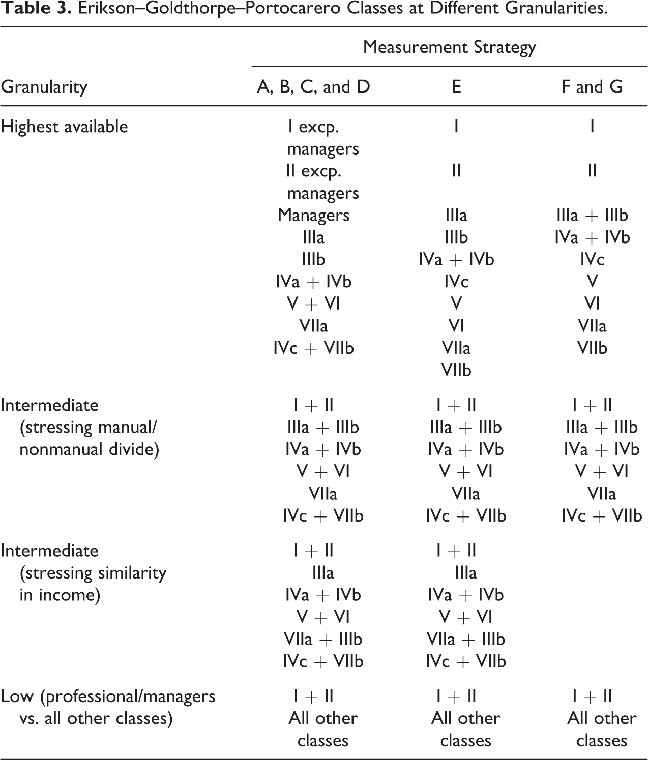
Strategies B through E all employ the internal indirect approach, using in all cases crosswalks generated by the U.S. Census Bureau (see Vines and Priebe 1989; Tables 1 and 2). We refer to these crosswalks as the 1970→1980 crosswalk (showing the 1980 COC distribution for each occupation in the 1970 COC) and the 1980→1970 crosswalk (defined analogously). Strategy B uses the 1970→1980 crosswalk to map the 1970 COC into the 1980 COC and then applies Hout’s mapping of the 1980 COC into EGP classes also used in strategy A. Strategy C proceeds in a similar way, but with the 1970 COC as the bridge classification: It uses the 1980→1970 crosswalk to map the 1980 COC into the 1970 COC and then uses Hout’s mapping of the 1970 COC into EGP classes. Strategy D is based on a mapping of the 1980 COC into EGP classes that was used in an auxiliary sensitivity analysis by Beller (2009:Ftn. 4); this mapping was also developed by Michael Hout.¹⁸ In Table 2, we refer to it as the Beller–Hout mapping. We combine it with the 1970→1980 crosswalk to map the 1970 COC into EGP classes. This measurement strategy was used by Mitnik et al. (2016). Table 3 shows that strategies B through D produce the same approximate EGP categories as strategy A.

Strategy E is based on the mapping from the 1980 COC into EGP classes developed by Morgan and Tang (2007). We combine it with the 1970→1980 crosswalk in order to map the 1970 COC into classes. A similar strategy was used by Weeden et al. (2007). Table 3 shows that, at its highest granularity, this strategy produces almost all of the classes in the full EGP scheme—the only exception being that classes IVa and IVb are collapsed into one class.

Finally, we examine two measurement strategies based on the external indirect approach. In both, the external classification used is the International Standard Classification of Occupations (ISCO). The ISCO is widely employed in cross-national research, as it was developed to give researchers a way to consistently classify occupations across countries. It has been revised several times, so to date, there are four versions: ISCO-58, ISCO-68, ISCO-88, and ISCO-08. The GSS recodes the 1970 COC into ISCO-68, and it recodes the 1980 COC into both ISCO-68 and ISCO-88.¹⁹

Ganzeboom and Treiman (e.g., 1996) have developed mappings from ISCO-68 and ISCO-88 into EGP classes; we will refer to these widely used mappings as GT-68 and GT-88. In her research with GSS data, Beller (2009) used the GSS’s 1980 COC→ISCO-88 recode and GT-88 to generate EGP classes, at an intermediate granularity, for the period 1994–2007.²⁰ We use a similar approach with measurement strategies F and G. Strategy F defines one mapping by combining the GSS’s 1980 COC→ISCO-88 recode and GT-88 and the other by combining the GSS’s 1970 COC→ISCO-68 recode and GT-68. Strategy G is similar but substitutes the GSS’s 1980 COC→ISCO-68 recode and GT-68 to define the first of the two mappings. Table 3 shows that, at their highest granularity, both strategies produce nine classes: Seven are classes from the full version of the EGP scheme, and the remaining two are aggregations of classes in that scheme (IIIa + IIIb and IVa + IVb).²¹

In addition to assessing the reliability of all measurement strategies at the highest granularity available, we also assess it at the intermediate granularity used in most empirical research. We consider two different ways of collapsing the full EGP scheme into six classes, which only differ in how they treat routine nonmanual employees, lower grade (IIIb; see Table 3).²² The first stresses the divide between manual and nonmanual workers, with all routine nonmanual workers grouped into one class (IIIa + IIIb). This way of collapsing EGP classes is very close to the widely used seven-class version (or CASMIN version) of the EGP scheme (Erikson and Goldthorpe 1992)—the only difference being that we assign all people working in agriculture to the same class, while the CASMIN version keeps farmers (IVc) and agricultural workers (VIIb) as two different classes.²³ We refer to this granularity as the “intermediate (manual/nonmanual) granularity.”

The second six-class version of the EGP scheme we consider includes all nonfarm lower-skill/lower-wage workers in one class, regardless of whether they are manual or nonmanual workers, by combining classes IIIb and VII (nonfarm semi- and unskilled manual workers). Mitnik et al. (2016) collapsed the EGP scheme in this way because prioritizing income similarities across classes rather than the manual/nonmanual divide was more appropriate for their goal of exploring the relationship between the post-1980 income-inequality take off and social fluidity in the United States. We refer to this granularity as the “intermediate (income-based) granularity.”

Finally, we assess the various measurement strategies at the minimum level of granularity that is possible, that is, when there are only two classes. Given recent arguments on the centrality of the divide between professionals and managers, and all other classes, for the study of trends (Mitnik et al. 2016), we focus here on a two-class version of the EGP scheme that only distinguishes classes I and II from all other classes.

Main Reliability Results

We present here the main results of our reliability analysis. As previously indicated, our analysis is based on the double-coded data in the 1988–1990 GSS. We constrain our sample to subjects ages 18–64 and estimate the reliability of EGP class measures for men and women separately, and for “all” (i.e., men and women pooled). We also estimate the reliability of measures of father’s class in two different ways.²⁴ In one case, we use the same EGP schemes that we use for men and women and drop all observations for which the father was absent from the household when the subject was 16 years old (the information on the subject’s father pertains to that age). In the other case, we add the category “nonresident father” to the EGP scheme. We refer to the resulting “population” as “fathers (expanded).” Table 4 shows the number of observations used to assess reliability in each case.²⁵

Table 4.

Number of Observations with Nonmissing Class Values.

Measurement Strategy	Population
Measurement Strategy	All	Men	Women	Fathers	Fathers (exp.)
A	3,314	1,530	1,784	2,904	3,389
B	3,293	1,510	1,783	2,858	3,343
C	3,316	1,532	1,784	2,909	3,394
D	3,289	1,506	1,783	2,856	3,341
E	3,282	1,502	1,780	2,838	3,323
F	3,302	1,514	1,788	2,881	3,366
G	3,329	1,539	1,790	2,931	3,416

Table 5 presents the point estimates of Krippendorff’s α (in boldface) and the corresponding confidence intervals (in square brackets).²⁶ The first three columns include the results for the EGP class of all respondents combined and of men and women separately. The last two columns show the results for fathers’ EGP class. Estimation of α is quite precise, so most of our discussion focuses on the point estimates.

Table 5.

Estimates of Krippendorff’s α.

Measurement Strategy	Measurement Granularity	Population
Measurement Strategy	Measurement Granularity	All	Men	Women	Fathers	Fathers (exp.)
A	High	.75 [.73, .77]	.73 [.70, .75]	.76 [.73, .78]	.73 [.71, .75]	.77 [.76, .79]
	Intermediate (manual/nonm.)	.77 [.75, .79]	.75 [.72, .78]	.78 [.75, .80]	.74 [.72, .76]	.78 [.77, .80]
	Intermediate (income)	.76 [.74, .78]	.74 [.71, .77]	.77 [.74, .80]	.74 [.72, .76]	.78 [.77, .80]
	Low	.77 [.75, .80]	.77 [.73, .80]	.77 [.74, .81]	.76 [.73, .79]	.84 [.82, .86]
B	High	.78 [.77, .80]	.78 [.76, .80]	.78 [.75, .80]	.78 [.77, .80]	.82 [.80, .83]
	Intermediate (manual/nonm.)	.81 [.79, .83]	.81 [.78, .83]	.80 [.77, .82]	.79 [.77, .81]	.83 [.81, .84]
	Intermediate (income)	.80 [.78, .81]	.80 [.77, .82]	.79 [.76, .81]	.79 [.77, .81]	.83 [.81, .84]
	Low	.79 [.77, .81]	.78 [.75, .82]	.80 [.77, .83]	.76 [.73, .78]	.84 [.82, .86]
C	High	.77 [.75, .78]	.75 [.73, .78]	.77 [.74, .79]	.79 [.77, .81]	.83 [.81, .84]
	Intermediate (manual/nonm.)	.81 [.79, .82]	.79 [.76, .82]	.81 [.78, .83]	.81 [.79, .83]	.84 [.83, .86]
	Intermediate (income)	.77 [.75, .79]	.77 [.74, .79]	.77 [.74, .80]	.80 [.78, .82]	.84 [.82, .85]
	Low	.79 [.76, .81]	.78 [.74, .81]	.79 [.76, .82]	.79 [.77, .82]	.86 [.84, .88]
D	High	.79 [.78, .81]	.80 [.78, .82]	.78 [.76, .81]	.83 [.82, .85]	.86 [.84, .87]
	Intermediate (manual/nonm.)	.82 [.80, .84]	.83 [.80, .85]	.80 [.77, .82]	.84 [.82, .86]	.87 [.85, .88]
	Intermediate (income)	.81 [.79, .82]	.82 [.79, .84]	.79 [.76, .81]	.84 [.82, .86]	.87 [.85, .88]
	Low	.81 [.79, .83]	.82 [.78, .85]	.80 [.77, .84]	.85 [.82, .87]	.90 [.89, .92]
E	High	.72 [.70, .74]	.70 [.67, .73]	.73 [.70, .75]	.75 [.73, .77]	.79 [.77, .81]
	Intermediate (manual/nonm.)	.80 [.78, .81]	.78 [.76, .81]	.80 [.77, .82]	.81 [.80, .83]	.85 [.83, .86]
	Intermediate (income)	.76 [.74, .77]	.75 [.72, .77]	.75 [.73, .78]	.80 [.78, .82]	.83 [.82, .85]
	Low	.77 [.74, .79]	.75 [.71, .79]	.78 [.75, .82]	.79 [.77, .82]	.86 [.85, .88]
F	High	.58 [.56, .60]	.58 [.55, .61]	.56 [.53, .59]	.62 [.60, .64]	.68 [.66, .70]
	Intermediate (manual/nonm.)	.66 [.64, .68]	.67 [.64, .70]	.63 [.59, .66]	.72 [.70, .74]	.77 [.76, .79]
	Low	.72 [.70, .75]	.72 [.68, .76]	.72 [.69, .76]	.72 [.69, .75]	.81 [.79, .83]
G	High	.69 [.67, .71]	.67 [.64, .70]	.69 [.66, .72]	.71 [.69, .73]	.76 [.74, .77]
	Intermediate (manual/nonm.)	.71 [.69, .73]	.69 [.66, .72]	.70 [.67, .73]	.73 [.71, .75]	.78 [.76, .80]
	Low	.75 [.73, .78]	.75 [.71, .79]	.76 [.72, .79]	.76 [.73, .78]	.84 [.82, .86]

Note: Point estimates are in boldface, 95% confidence intervals are in square brackets.

The estimated values of α exhibit a great deal of variability—they span the range .56 to .90, with a mean of .77 and a median of .78. They also show clear patterns across strategies. Some of these patterns are particularly apparent in Figure 4, where we use different colors and shapes to distinguish the values of α according to the approach of the corresponding measurement strategy and display those values separately for all respondents, men, women, fathers, and fathers (expanded) at each granularity.

Figure 4.

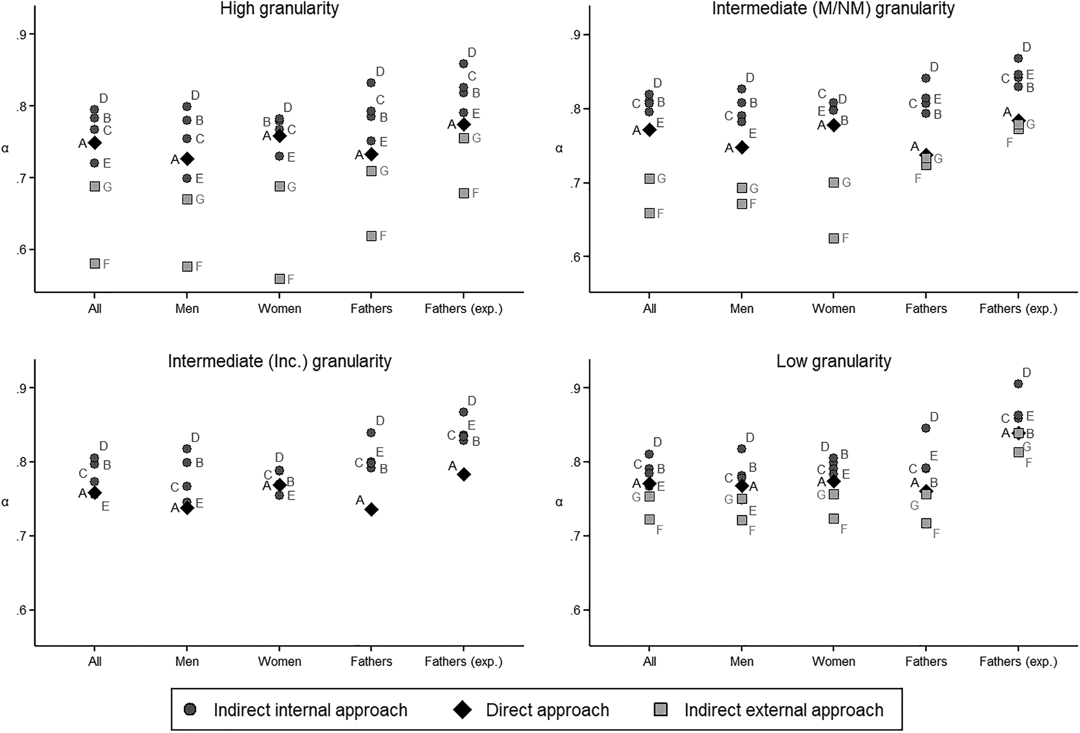
Krippendorff’s α by granularity and approach.

The most important of these patterns is the near-perfect ordering of the strategies—within population-granularity pairs—by approach, with those strategies using the internal indirect approach (B, C, D, and E) outperforming all others in nearly every case, and the strategy using the direct approach (A) never outperformed by (and mostly outperforming) those using the external indirect approach (F and G). For the intermediate (manual/nonmanual) granularity (the granularity most often employed in empirical research), the seven strategies are perfectly ordered by approach regardless of population. At the other three granularities, the pattern is very similar, though in some cases, strategy A outperforms strategy E.

What drives the ordering of the strategies by approach? To answer, we need to distinguish between two types of mappings between classifications. There are mappings that are generated through a fully objective procedure, such as those based on the 1970→1980 and 1980→1970 crosswalks. The crosswalks result from a simple cross tabulation of a double-coded data set. Once the double-coded data on which a crosswalk is based are available, the associated mapping could be fully generated—at least in principle—by a computer program. Therefore, we may refer to mappings like this as “mechanical mappings.” In contrast, there are mappings that rely in an essential way on a researcher’s judgment regarding the relationship between the categories in two classifications, as is the case with all mappings from occupational classifications into EGP classes. Although these mappings are based on objective facts that clearly constrain which occupations may be reasonably mapped into which EGP classes, they involve an unavoidable element of discretionary subjective judgment. We may refer to these mappings as “nonmechanical mappings.”

Our hypothesis is that, within granularity-population pairs, reliability performance is mostly accounted for by the number of nonmechanical mappings a measurement strategy relies upon. Or, in other words, that reliability performance is largely accounted for by the extent to which a strategy relies on subjective judgments regarding relationships between classifications.

The strategies based on the internal indirect approach (which we found to produce the most reliable class measures) use only one nonmechanical mapping—the mapping of one occupational classification into EGP classes. Here, the second occupational classification is mapped into the first through a mechanical mapping and then mapped into classes using the same nonmechanical mapping employed with the first classification.²⁷ The direct approach, in contrast, involves two nonmechanical mappings because each occupational classification is mapped separately into classes. The one strategy we consider that is based on the direct approach, strategy A, is consistently outperformed by the four strategies based on the internal indirect approach.

The strategies we examine that use the external indirect approach involve even more nonmechanical mappings: Strategy F uses four while strategy G uses three. (Strategy F uses nonmechanical mappings of the two COCs into two different ISCOs and then uses two nonmechanical mappings to map the ISCOs into EGP classes. Strategy G differs only in that it maps both COCs into the same ISCO, so it requires only one ISCO→EGP mapping.) Consistent with our hypothesis that reliability is closely related to the number of nonmechanical mappings employed, these two strategies are consistently the least reliable of our seven, and F performs substantially worse than strategy G. Indeed, strategy F has the lowest reliability of all strategies, for all populations. This is the case for all granularities at which this strategy can be implemented, but most notably at the high measurement granularity, where its performance is about two standard deviations below the mean.²⁸

In addition to the ordering of strategies by approach, some granularity-related patterns are apparent. Table 5 and Figure 4 show that, regardless of strategy, there is in nearly all cases a gain in reliability (and never a loss) when switching from the high granularity to the other granularities. As Krippendorff’s α does take into account that chance agreement is more likely as the granularity of a measure falls, this pattern reflects a real reliability penalty attached to working with high-granularity measures. At the same time, the reliability gains from switching from the high to the low granularity are only substantial for strategies E, G, and F and are largest for the latter (which, as indicated, performs very poorly at the high granularity). Moreover, for the best-performing strategies (B, C, and D), reliability at the intermediate granularities tends to be higher than at both the high and the low granularities, although only slightly so in most cases. For five of the seven strategies, we can also compare the values of α across the two intermediate granularities. Table 5 indicates that the class measure is less reliable at the intermediate (income-based) granularity than at the intermediate (manual/nonmanual) granularity in the case of strategies C and E, while the differences are either nil or negligible in the other cases.

For the most part, there are only small differences in reliability across “generations” (men versus fathers). When nonresident fathers are included, the values of α for fathers are quite substantially larger than those for men (Figure 4 and Table 5), but this is only because there is always agreement across mappings when nonresident fathers are added as a separate category. When nonresident fathers are excluded from the analysis, the values of α for fathers tend to be slightly smaller than those for men in the case of strategies A and B and slightly larger otherwise.

Gender does not seem to make any difference, that is, Table 5 does not suggest any consistent gender advantage in reliability. The values of α tend to be slightly higher for women than for men in strategies A, C, E, and G, the other way around in strategies D and F, with gender differences varying in sign across granularities in the case of strategy B.

Table 6 reports the results of a linear regression of α on the number of nonmechanical mappings (entered as a nominal variable), granularity, gender, and generation. All estimates are consistent with the patterns identified in our qualitative analysis. In particular, the coefficients for two, three, and four nonmechanical mappings are all negative, substantial in magnitude, and statistically significant. The value of the adjusted $R^{2}$ indicates that about four fifths of the observed variation in α is accounted by the explanatory factors included in the regression.²⁹

Table 6.

Linear Regression of Krippendorff’s α on Number of Nonmechanical Mappings, Granularity, Gender, and Generation.

	Krippendorff’s α
Number of nonmechanical mappings
Two	−.04**
Three	−.07**
Four	−.12**
Granularity
Intermediate (manual/nonmanual)	.04**
Intermediate (income based)	.03**
Low	.05**
Gender
All (men and women)	.01
Women	.00
Generation
Father	.02*
Father (expanded)	.07**
Constant	.75**
Observations	130
Adjusted R ²	.78

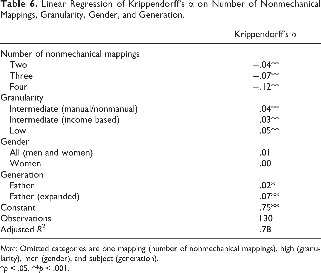
Note: Omitted categories are one mapping (number of nonmechanical mappings), high (granularity), men (gender), and subject (generation).

*p < .05. **p < .001.

We finish our main reliability analysis by presenting, in Table 7, the results of testing the null hypothesis that the value of α is not larger than .75 for each measurement strategy, at each granularity and for each population we consider. We use .75 as a threshold for an “acceptable” level of reliability; this value is in line with thresholds that have been used in several other related contexts.³⁰ If the null hypothesis is rejected, we can be reasonably confident that a measurement strategy produces class measures that are reliable enough to be employed in empirical analyses.

Table 7.

Hypothesis Tests for Krippendorff’s α ≤ .75.

Measurement	Measurement	Population
Strategy	Granularity	All	Men	Women	Fathers	Fathers (exp.)
A	High					**
	Intermediate (M/NM)	*		*		***
	Intermediate (Inc.)					***
	Low	*				***
B	High	***	**	**	***	***
	Intermediate (M/NM)	***	***	***	***	***
	Intermediate (Inc.)	***	***	**	***	***
	Low	***	*	**		***
C	High	*			***	***
	Intermediate (M/NM)	***	**	***	***	***
	Intermediate (Inc.)	**			***	***
	Low	**		**	***	***
D	High	***	***	**	***	***
	Intermediate (M/NM)	***	***	***	***	***
	Intermediate (Inc.)	***	***	**	***	***
	Low	***	***	***	***	***
E	High					***
	Intermediate (M/NM)	***	**	***	***	***
	Intermediate (Inc.)				***	***
	Low			*	***	***
F	High
	Intermediate (M/NM)					**
	Low					***
G	High
	Intermediate (M/NM)					***
	Low					***

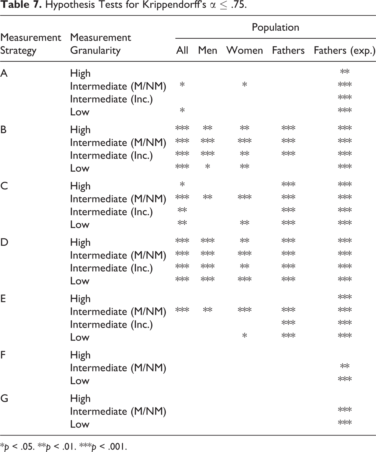
*p < .05. **p < .01. ***p < .001.

This table underscores again that the strategies based on the internal indirect approach (strategies B through E) produce class measures that are clearly superior in their reliability to strategies based on the other approaches. Strategies B and D perform particularly well. For the latter, the null hypothesis can be rejected for all granularities and populations; for the former, it can be rejected for all granularities and populations except one. For the strategies using the external indirect approach—F and G—the null cannot be rejected for any population, regardless of granularity (ignoring the expanded scheme for fathers). Strategy A, which uses the direct approach, falls somewhere in between.

At the highest level of granularity—and again ignoring the expanded scheme for fathers—the null can only be rejected for the best-performing strategies (i.e., B, C, and D). At the intermediate manual/nonmanual granularity most often used in empirical research, the null is very clearly rejected for all populations when using strategies B, C, D, and E (all of which are based on the indirect internal approach and use only one nonmechanical mapping), but not with the other strategies.

Illustrative Analysis: The Core Model of Social Fluidity

The “core model of social fluidity,” developed by Erikson and Goldthorpe (1992), is used widely in the field of intergenerational class mobility (see, e.g., Breen 2004). We estimate it here for men ages 31–64, using the double-coded data from the GSS 1988–1990 we employed in our previous analyses.³¹ For each of our seven measurement strategies, we estimate the same model twice, once using the EGP class measure based on the 1970 COC and once using the class measure based on the 1980 COC. We use class measures at the intermediate (manual/nonmanual) granularity. This illustrative analysis will allow us to show that the extent to which results differ within measurement strategies (that is, across occupational classifications) is strongly related to their reliability performance as measured by Krippendorff’s α.

The reliability estimates for the sample used in the analysis are presented in Table 8. The table includes estimates of α for the EGP class of men ages 31–64 and for the EGP class of their fathers (as well as the corresponding p values for the null hypothesis that $α \leq .75$ ). In the context of content analysis, Krippendorff (2013:326) has argued that “it is a serious mistake to average the reliabilities of the variables of a complex instrument and take this average as a measure of overall data reliability…[g]enerally, when variables are equally important to the research effort…the lowest α among them is the reliability of all data” (italics omitted). This suggests using the minimum of men’s and their fathers’ α (or “minimum α”) as the relevant measure of reliability when comparing strategies. This is what we do below.

Table 8.

Estimates of Krippendorff’s α, Core-Model Class Variables (Men Ages 31–64).

Measurement	Number of Observations	Men’s		Men’s Fathers
Strategy	Number of Observations	α	p Value	α	p Value
A	935	.72 [.68, .76]	.934	.72 [.68, .75]	.961
B	913	.79 [.76, .82]	.011	.79 [.76, .82]	.007
C	940	.76 [.73, .80]	.221	.79 [.76, .82]	.007
D	909	.81 [.78, .84]	.000	.82 [.79, .85]	.000
E	904	.76 [.72, .80]	.308	.81 [.78, .84]	.000
F	924	.67 [.63, .71]	1.000	.72 [.69, .76]	.949
G	951	.68 [.64, .72]	1.000	.73 [.70, .76]	.869

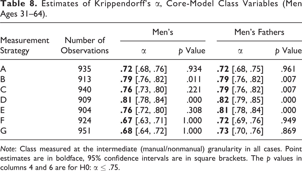
Note: Class measured at the intermediate (manual/nonmanual) granularity in all cases. Point estimates are in boldface, 95% confidence intervals are in square brackets. The p values in columns 4 and 6 are for H0: α ≤ .75.

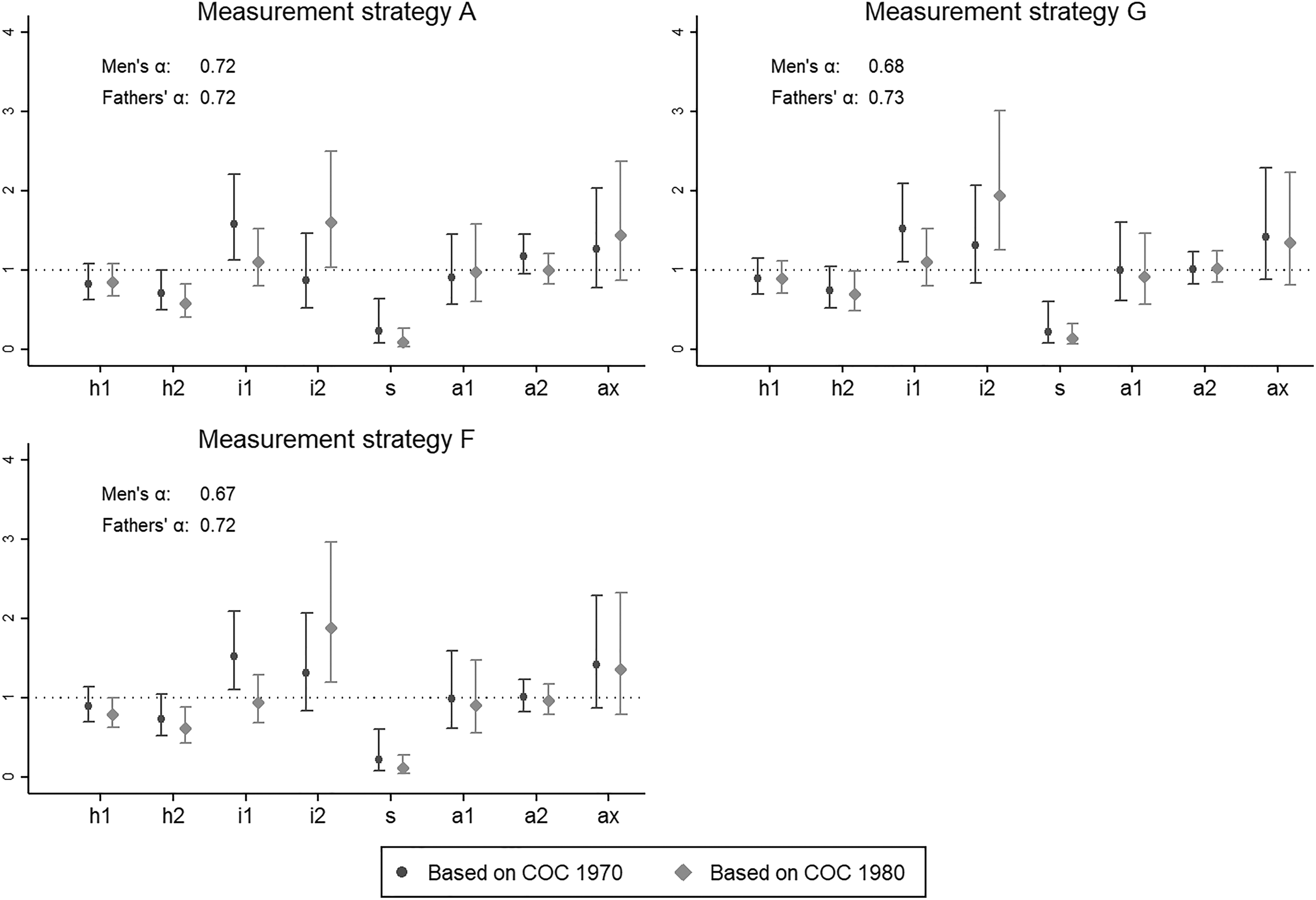
We estimate the “U.S. variant” of the core model of social fluidity (Erikson and Goldthorpe 1992:121-31, 318-9). As the model is very well known, we will not present it in any detail here. However, to facilitate understanding of the discussion that follows, we remind the reader that this is a log-linear, or multiplicative, model of the cells of a mobility table (i.e., a cross tabulation of the subject’s and his father’s EGP class) and that the predicted quantities in the model are the expected frequencies in each cell of that table. We will focus on eight key parameters: Parameters h1 and h2, which aim to capture the effects on relative-mobility patterns of barriers to movements across classes at different hierarchical levels; parameters i1 and i2, which reflect the tendency of sons to inherit the class position of their fathers; parameter s, which measures barriers to movements between agricultural and nonagricultural class positions; and parameters a1, a2, and ax, which measure affinity among class positions. We refer to these eight parameters as “model-specific parameters.” As is standard in models of relative mobility based on mobility tables, the core model also includes other parameters aimed at capturing the main effects of the distribution of individuals over origin and destination classes and the scale of the table.³²

Figures 5a and 5b display, for each measurement strategy, a graph with the estimates of the model-specific parameters with the two EGP measures.³³ The darker bars show the parameter estimates using the class measure based on the 1970 COC; the lighter bars show the estimates using the class measure based on the 1980 COC. The strategies are arranged in decreasing order of reliability (as measured by their minimum α)—that is, the first graph corresponds to the strategy with the highest reliability, the second graph to the strategy with the second-highest reliability, and so forth. The first two graphs are those for strategies D and B, whose minimum α is close to .8. For these strategies with relatively high reliability, the estimates based on the 1970 and 1980 COCs are extremely similar (although clearly not identical). At the other end of the spectrum, the graphs for strategies A, G and F, whose minimum α is in the .67 to .72 range, show large within-graph discrepancies in the estimates of the inheritance parameters i1 and i2 (other discrepancies are similar in magnitude to those found in the case of strategies D and B). Importantly, the differences between the estimated inheritance parameters are very consequential for the qualitative conclusions that can be drawn. For instance, if i1 is equal to one, that means that—once all other forces included in the model are considered—sons are not more likely to be found in the same class positions as their fathers. The null hypothesis that this is the case cannot be rejected if the confidence interval for the parameter includes one. With strategies A, G, and F, the confidence interval covers the value one with one occupational classification but not with the other. Not rejecting the null would go against “one of the most secure findings of mobility research” (Erikson and Goldthorpe 1992:125).

Figure 5a.

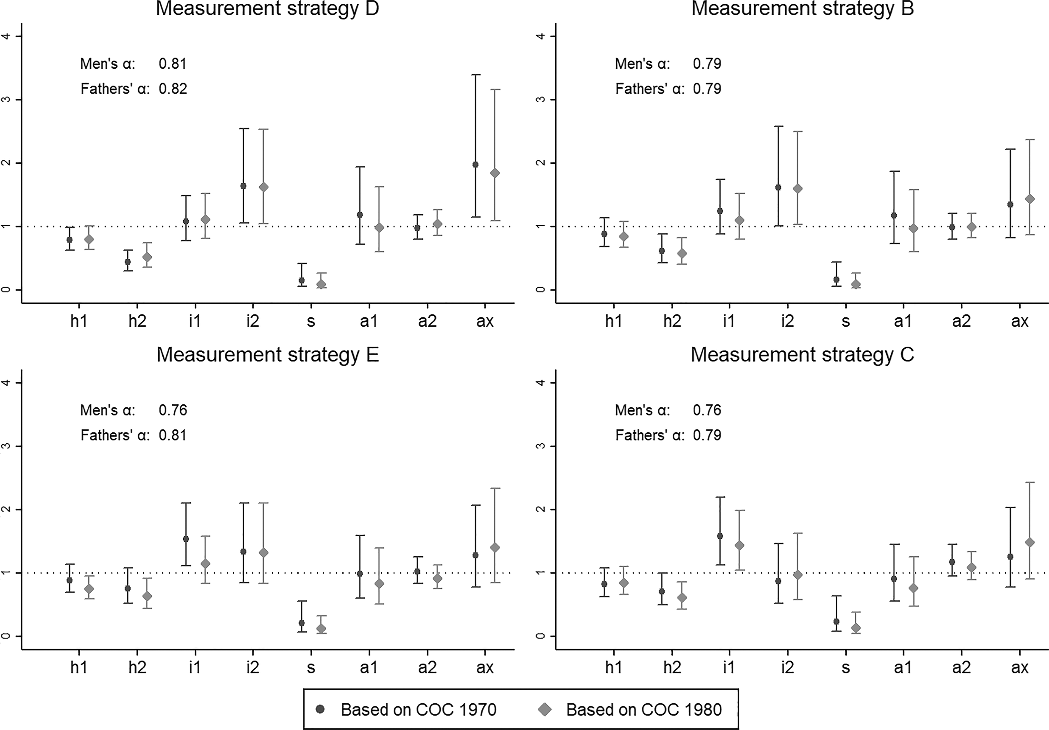
Core-model parameter estimates (model-specific parameters).

The graphs for strategies E and C, whose minimum α is .76 in both cases, indicate that the magnitude of discrepancies for these cases is in between those found for the other two groups. Thus, considered jointly, the estimates in Figures 5a and 5b reveal a clear correspondence between reliability levels and qualitative assessments of the consistency of the estimates across occupational classifications.

For some purposes, researchers may care about the operation of the full model rather than about specific parameters. In this context, one way of assessing how much the estimates of the model as a whole differ across occupational classifications is by defining loss functions whose arguments are the differences in predicted frequencies in the cells of the mobility table. These loss functions capture the net effect of differences in the estimates of all parameters at once. The expectation is that we will observe again a clear correspondence between reliability and the losses defined by these loss functions.

As table totals vary slightly across measurement strategies, it is more convenient to work with predicted relative frequencies than with predicted frequencies (which are the quantities directly predicted by the model). To carry out the analysis, we define four loss functions that vary in two dimensions: (a) whether they measure the distance between predicted values as absolute differences or as absolute proportional differences and (b) whether they use the arithmetic mean or the median as summary measure of the observed differences.³⁴ The resulting loss functions are thus the mean and median absolute differences in predictions, and the mean and median absolute proportional differences in predictions, across occupational classifications.³⁵ We will refer to the losses defined by these four loss functions as “prediction losses.”

Figure 6 presents plots of the prediction losses against the minimum α. It includes one graph for each loss function, with the loss in the vertical axis and the minimum α in the horizontal axis. For all loss functions, there is a clear negative relationship between the values of α and the size of the losses, with the dots representing the most reliable strategies clustered in the right-bottom quadrant of the graphs, and those representing the other strategies appearing in the left-upper quadrant. Spearman rank correlations are negative and large in all cases, that is, their absolute values are in the .71 to .79 range. The expectation of a clear correspondence between values of α and prediction losses is borne out by these results.

Figure 5b.

Core-model parameter estimates (model-specific parameters).

Figure 6.

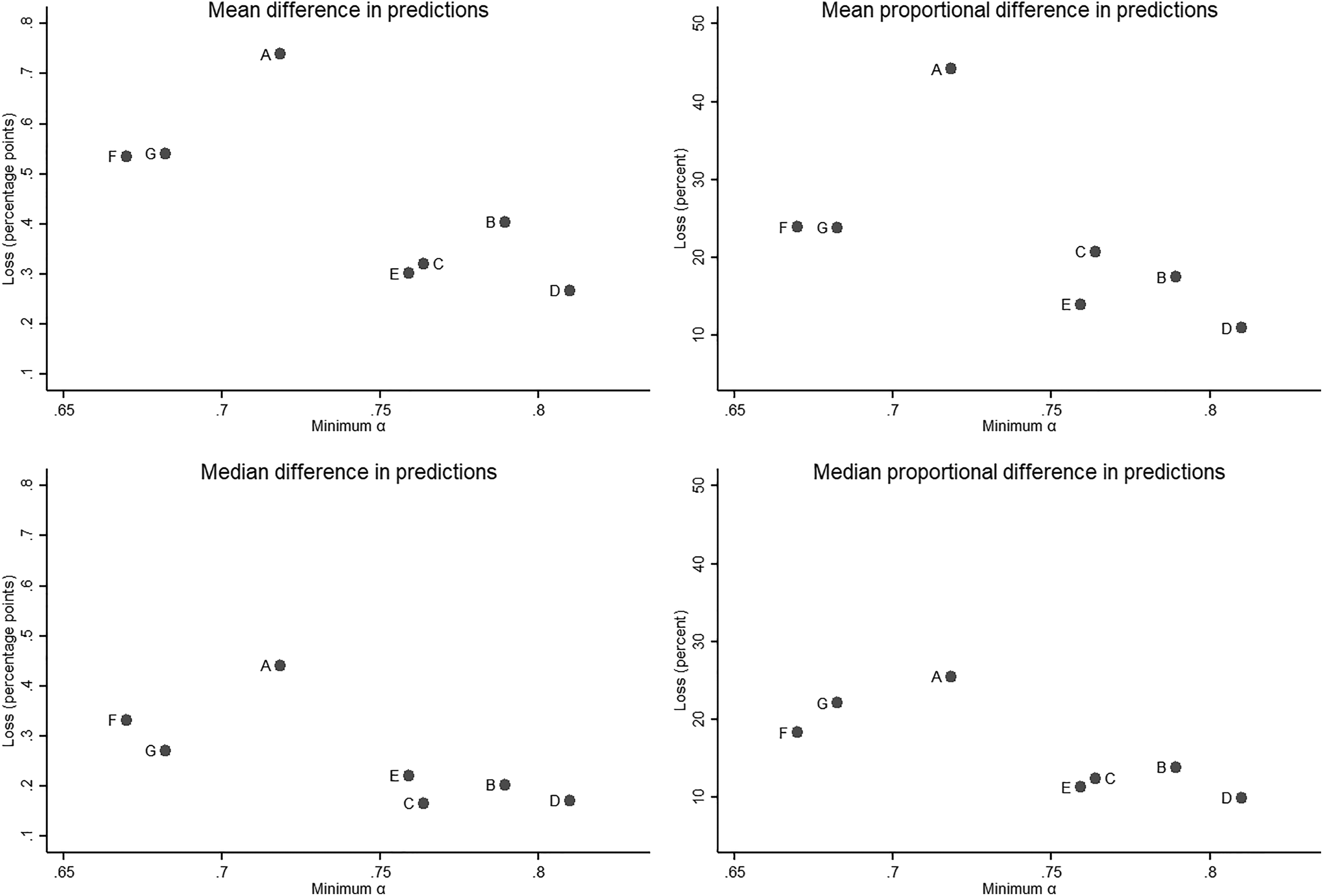
Core-model prediction losses as a function of Krippendorff’s α.

Figure 6 also indicates that for the best-performing strategy in terms of reliability (strategy D), the mean and median differences in predicted relative frequencies are smaller than .3 and .2 percentage points, respectively. The proportional differences are also small, around 10 percent. The other three strategies with reliability above .75 (B, C, and E) do not do as well as D—but they do not do much worse either, especially in terms of the median loss functions, which are much more robust to outlier differences. Among the three strategies with lower reliability values—all of which tend to post much larger losses—strategy A performs much worse than F and G, in spite of a larger minimum α. The reason for this is that with strategy A, the disagreements in coded EGP classes across the 1970 and 1980 COCs are disproportionally concentrated in one category, nonfarm self-employment (disagreements are much more evenly distributed with all other strategies). This has a large impact on the estimates of the main effects of the distribution of individuals over origin and destination classes, which translates into much larger differences in predicted frequencies.³⁶

Discussion

Our case study has made clear that measurement strategies that may seem equally sensible a priori differ markedly in the reliability of the class measures they generate. At the crucial intermediate (manual/nonmanual) granularity used most often in empirical research, reliability, as measured by Krippendorff’s α, is between 13 and 27 percent higher with the best-performing measurement strategy than with the worst-performing one (with the exact figure depending on the population). The reliability differential is even higher at the high granularity, where α is between 26 and 38 percent higher with the best performer.

Crucially, there seems to be a simple logic to the reliability differences observed within granularity-population pairs, as the variation in performance among the seven strategies is largely accounted by the number of nonmechanical mappings they employ. Thus, the analysis suggests that the fewer “researcher degrees of freedom” that go into defining a measurement strategy, the more reliable the data tend to be.

The case study has uncovered trade-offs between reliability and granularity, but these are somewhat complex. Although it is the case that the lower the granularity the higher the percentage of agreements across occupational classifications, it is not the case that, in general, the lower the granularity the higher the reliability of the data. For nearly all populations and measurement strategies, there are reliability penalties associated with measuring at a high granularity compared to measuring at both the intermediate and low granularities. However, there is no consistent penalty for measuring at the intermediate granularities compared to measuring at the low granularity, as in this case reliability only increases consistently across populations for the worst performers, while it often falls or stays the same for the more reliable strategies. Lastly, all granularity penalties tend to be rather small with the best-performing strategies.

We examined two different ways of collapsing the full EGP scheme into an intermediate granularity. Mitnik et al. (2016) have argued that the standard way of collapsing EGP categories in empirical analyses—that is, the CASMIN version of the EGP scheme, which is similar to our intermediate (manual/nonmanual) granularity—is, for some purposes, conceptually less appealing than an approach that prioritizes income similarities across classes rather than the manual/nonmanual divide. Our results indicate that there is a nonnegligible reliability cost from using the income-based approach with two of the five strategies for which we could compare the approaches, but not with the other three.

Our illustrative analysis focused on the core model of social fluidity and showed a clear correspondence between values of α and qualitative assessments of the consistency of the estimates of its model-specific parameters across occupational classifications. A quantitative, and more holistic, assessment based on prediction losses also indicated correspondence. It showed a clear separation of the measurement strategies into two groups, with those with reliability lower than .75 tending to post much larger losses, and with the associated rank correlations between prediction losses and values of α all above .7 and some close to .8. These results provide reassurance that α works as expected.

At the same time, in the analysis of prediction losses, within-group ranks based on the minimum α do not match well the corresponding ranks based on losses. This is particularly the case for the lower-reliability group, in which strategy A performs substantially worse than strategies F and G despite its higher α. Other empirical analyses, whose results we did not include here to save space, exhibit similar patterns. This suggests that researchers should not use values of α to mechanically rank measurement strategies, but rather should use them to (a) discard strategies that are below some minimum value deemed acceptable, (b) among those strategies that are acceptable, only use values of α to rank strategies (in terms of their reliability) if the differences between those values are substantial, and (c) report the value of α for the measures actually used in their empirical analyses.

What may be deemed an acceptable value of α? Based on threshold values used in related contexts (see note 30) and on the results of our empirical analyses, we suggest that, as a rule of thumb, a class measure be judged acceptable if the null hypothesis that $α \leq .75$ is rejected at the conventional significance level. And that, when comparing strategies for which this null hypothesis can be rejected, only differences in the value of α of about .04 or larger be considered informative. In spite of the fact that our acceptability criterion may seem somewhat conservative, the class variables generated by four of the measurement strategies we examined satisfy it for all populations (Table 7). In the case of the data used in our illustrative study (men ages 31–64 and their fathers), Table 8 indicates that strategies B and D satisfy the criterion for both the subject- and the father-class variables (with strategies C and E satisfying it for the father but not for the subject).

Conclusions

Periodic changes in occupational classifications may be a serious obstacle for conducting research on class-based trends. The magnitude of the problem, however, depends not only on the nature and scope of the changes but also on the measurement strategies used to address them. We have proposed here that scholars interested in conducting research on class-based trends use Krippendorff’s α to assess the reliability of class measures generated from data coded using different occupational classifications.

This reliability index has many desirable properties. It does not conflate predictability with agreement in class values. It takes into account that agreement may occur by chance, using for this purpose a methodologically appealing conception of chance. It has a range of variation with clear reliability interpretations. It may be computed regardless of the metric of the class variable. It may be legitimately used to compare measurement strategies across class schemes, metrics, and granularities, which allows evaluation of various reliability-related trade-offs (for instance, from working at a higher rather than at a lower granularity or from using one class scheme rather than another). Lastly, coincidence-matrix formulas typically used to simplify computation also allow straightforward estimation and statistical inference—based not in the resampling approaches employed in the reliability literature but in the much less time- and computer-intensive delta method—even in the context of complex sampling designs. For nominal variables, a computer program made available as a companion to the paper, and which implements the approach for statistical inference suggested here, makes both estimation and inference very simple and fast endeavors.

We put Krippendorff’s α to work in conducting a case study of the effects of the switch from the 1970 to the 1980 U.S. COC on the reliability of EGP class measures. We found that the reliability of EGP class measures varies substantially across measurement strategies that, a priori, seem equally sensible. In addition, our analysis showed that the main driving force behind that variation is the extent to which researchers’ subjective judgments play a role in defining a strategy. These results suggest general lessons that can be expected to apply to research on class-based trends regardless of its national and temporal context.

Class scholars have maintained that the discontinuity resulting from the switch in occupational classifications in the United States has made it very difficult, if not impossible, to consistently measure social class across the 1970–1980 divide, in particular with the EGP class scheme. The results of our case study indicate, however, that as long as the right measurement strategies are employed, the problems generated by that switch are substantially less consequential than previously argued. The best-performing strategies appear to produce data reliable enough to study class-based trends, in particular at the intermediary level of granularity typically used in empirical research. Given that in most cases the replacement of an old occupational classification by a new one involves a more limited conceptual and empirical break than the one we have considered here, our results suggest that well-chosen measurement strategies should generally produce data reliable enough for the study of class-based trends with data sets coded partly with one occupational classification and partly with a different, temporally contiguous, classification.

Supplemental Material

Supplemental Material, Mitnik_Cumberworth_Replication_package - Measuring Social Class with Changing Occupational Classifications: Reliability, Competing Measurement Strategies, and the 1970–1980 U.S. Classification Divide

Supplemental Material, Mitnik_Cumberworth_Replication_package for Measuring Social Class with Changing Occupational Classifications: Reliability, Competing Measurement Strategies, and the 1970–1980 U.S. Classification Divide by Pablo A. Mitnik and Erin Cumberworth in Sociological Methods & Research

Footnotes

Acknowledgment

The authors would like to thank Emily Beller and Michael Hout for sharing several algorithms they developed and used in their research to map occupations and other variables into Erikson–Goldthorpe–Portocarero classes.

Declaration of Conflicting Interests

The author(s) declared no potential conflicts of interest with respect to the research, authorship, and/or publication of this article.

Funding

The author(s) received no financial support for the research, authorship, and/or publication of this article.

Supplemental Material

Supplemental material for this article is available online.

Notes

References

Beller

Emiliy

. 2009. “Bringing Intergenerational Social Mobility Research Into the Twenty-first Century: Why Mothers Matter.” American Sociological Review 74(4):507–28.

Bennett

Alpert

Goldstein

. 1954. “Communications Through Limited-response Questioning.” Public Opinion Quarterly 18(3):303–8.

Breen

Richard

(Ed.). 2004. Social Mobility in Europe. Oxford, England: Oxford University Press.

Brennan

R. L.

Prediger

D. J.

. 1981. “Coefficient Kappa: Some Uses, Misuses, and Alternatives.” Educational and Psychological Measurement 41:687–99.

Carmines

Edward

Zeller

Richard

. 1979. Reliability and Validity Assessment. London, England: Sage.

Cohen

1960. “A Coefficient of Agreement for Nominal Scales.” Educational and Psychological Measurement 20:37–46.

Cronbach

L. J.

1951. “Coefficient Alpha and the Internal Structure of Tests.” Psychometrica 16:297–334.

Erikson

Robert

Goldthorpe

John

. 1992. The Constant Flux: A Study of Class Mobility in Industrial Societies. New York: Oxford University Press.

Fleiss

Joseph L.

Levin

Bruce

Paik

Myunghee Cho

. 2003. Statistical Methods for Rates and Proportions. New York: Wiley.

10.

Ganzeboom

Harry

Treiman

Donald

. 1996. “Internationally Comparable Measures of Occupational Status for the 1988 International Standard Classification of Occupations.” Social Science Research 25:201–39.

11.

Goldthorpe

John

. 2000. On Sociology: Numbers, Narratives and the Integration of Research and Theory. Oxford, England: Oxford University Press.

12.

Hauser

Robert

. 1998. “Intergenerational Economic Mobility in the United States. Measures, Differentials and Trends.” CDE Working Paper No 98-12, Center for Demography and Ecology, University of Wisconsin-Madison.

13.

Hayes

Andrew

Krippendorff

Klaus

. 2007. “Answering the Call for a Standard Reliability Measure for Coding Data.” Communication Methods and Measures 1(1):77–89.

14.

Heeringa

S. G.

West

B. T.

Berglund

P. A.

. 2010. Applied Survey Data Analysis. Boca Raton, FL: Chapman & Hall/CRC.

15.

Hout

Michael

. 2005. “Educational Progress for African-Americans and Latinos in the United States from the 1950s to the 1990s: The Interaction of Ancestry and Class.” Pp. 262–87 in Ethnicity, Social mobility and Public Policy: Comparing the USA and UK, edited by Loury

Glenn

Modood

Tariq

Teles

Steven Michael

. Cambridge, England: Cambridge University Press.

16.

Hsu

Louis

Field

Ronald

. 2003. “Interrater Agreement Measures: Comments on Kappa_n, Cohen’s Kappa, Scott’s π, and Aickin’s α.” Understanding Statistics 2(3):205–19.

17.

Krippendorff

Klaus

. 1970. “Bivariate Agreement Coefficients for Reliability of Data.” Sociological Methodology 2:139–50.

18.

Krippendorff

Klaus

. 2004. “Reliability in Content Analysis. Some Common Misconceptions and Recommendations.” Human Communication Research 30(3):411–33.

19.

Krippendorff

Klaus

. 2011. “Computing Krippendorff’s Alpha-reliability.” Retrieved July 10, 2013. (http://web.asc.upenn.edu/usr/krippendorff/mwebreliability5.pdf).

20.

Krippendorff

Klaus

. 2013. Content Analysis: An Introduction to its Methodology. 3rd ed. Los Angeles, CA: Sage.

21.

Krippendorff

Klaus

. [2006] 2016. “Bootstrapping Distributions for Krippendorff’s Alpha.” Retrieved November 7, 2016. (http://web.asc.upenn.edu/usr/krippendorff/boot.c-Alpha.pdf).

22.

McCall

Leslie

Manza

Jeff

. 2011. “Class Differences in Social and Political Attitudes in the United States.” Pp. 552–70 in The Oxford Handbook of American Public Opinion and the Media, edited by

Jacobs

Lawrence R.

Edwards

George C.

Shapiro

Robert Y.

23.

Mielke

Paul

Berry

Kenneth

. 2001. Permutation Methods: A Distance Function Approach. New York: Springer.

24.

Mitnik

Pablo

Cumberworth

Erin

Grusky

David

. 2016. “Social Mobility in a High-inequality Regime.” The Annals of the American Academy of Political and Social Science 663(1):140–84.

25.

Morgan

Stephen

Cha

Youngjoo

. 2007. “Rent and the Evolution of Inequality in Late Industrial United States.” American Behavioral Scientist 50(5):677–701.

26.

Morgan

Stephen

McKerrow

Mark

. 2004. “Social Class, Rent Destruction, and the Earnings of Black and White Men, 1982–2000.” Research in Social Stratification and Mobility 21:215–51.

27.

Morgan

Stephen

Tang

Zun

. 2007. “Social Class and Workers’ Rent, 1983–2001.” Research on Social Stratification and Mobility 25:273–93.

28.

Nunnally

J. C.

Bernstein

I. H.

. 1994. Psychometric Theory. New York: McGraw-Hill.

29.

Oehlert

Gary

. 1992. “A Note on the Delta Method.” The American Statistician 46(1):27–29.

30.

Pfeffer

Fabian

Hertel

Florian

. 2015. “How Has Educational Expansion Shaped Social Mobility Trends in the United States?” Social Forces 94(1):143–80.

31.

Scott

William

. 1955. “Reliability of Content Analysis. The Case of Nominal Scale Coding.” Public Opinion Quarterly 19:321–25.

32.

Shrout

Patrick

. 1998. “Measurement Reliability and Agreement in Psychiatry.” Statistical Methods in Medical Research 7:301–17.

33.

Sijtsma

Klaas

. 2009. “On the Use, the Misuse, and the Very Limited Usefulness of Cronbach’s Alpha.” Psychometrica 74(1):107–20.

34.

Skinner

C. J.

Holt

Smith

T. M. F.

(eds.). 1989. Analysis of Complex Surveys. New York: Wiley.

35.

Smith

Tom W.

Marsden

Peter H.

Hout

Michael

Jibum

Kim

. 2011. General Social Surveys, 1972–2010 [machine-readable data file]. Chicago, IL: National Opinion Research Center.

36.

Vines

Paula L.

Priebe

John A.

. 1989. The Relationship Between the 1970 and 1980 Industry and Occupation Classification Systems. Washington, DC: U.S. Bureau of the Census.

37.

Warrens

Matthijs

. 2012. “The Effects of Combining Categories on Bennett, Alpert and Goldstein’s S.” Statistical Methodology 9:341–52.

38.

Weeden

Kim

Young-Mi

Carlo

Matthew Di

Grusky

David

. 2007. “Social Class and Earnings Inequality.” American Behavioral Scientist 50:702–36.

39.

Weeden

Kim

Grusky

David

. 2004. “Are There Any Big Classes at All?” Research in Social Stratification and Mobility 22:3–56.

40.

Wright

Erik Olin

Martin

Bill

. 1987. “The Transformation of the American Class Structure, 1960–1980.” American Journal of Sociology 93(1):1–29.

41.

Zwick

Rebecca

. 1988. “Another Look at the Inter-rater Agreement.” Psychological Bulletin 103(3):374–87.

Supplementary Material

Please find the following supplemental material available below.

For Open Access articles published under a Creative Commons License, all supplemental material carries the same license as the article it is associated with.

For non-Open Access articles published, all supplemental material carries a non-exclusive license, and permission requests for re-use of supplemental material or any part of supplemental material shall be sent directly to the copyright owner as specified in the copyright notice associated with the article.

24.68 MB

0.00 MB

Measuring Social Class with Changing Occupational Classifications: Reliability,Competing Measurement Strategies,and the 1970–1980 U.S. Classification Divide

Abstract

Keywords

Introduction

Reliability and Social-Class Measurement Strategies

Critical Assessment of Widely Used Reliability Indices

Krippendorff’s α

Krippendorff’s α with Nominal Class Variables: Computation and Statistical Inference

Case Study: Bridging the 1970–1980 U.S. Occupational Classification Divide

The EGP Class Scheme

Measurement Strategies

Main Reliability Results

Illustrative Analysis: The Core Model of Social Fluidity

Discussion

Conclusions

Supplemental Material

Supplemental Material, Mitnik_Cumberworth_Replication_package - Measuring Social Class with Changing Occupational Classifications: Reliability, Competing Measurement Strategies, and the 1970–1980 U.S. Classification Divide

Footnotes

Acknowledgment

Declaration of Conflicting Interests

Funding

Supplemental Material

Notes

References

Supplementary Material