Anything Lorenz Curves Can Do,Top Shares Can Do: Assessing the TopBot Family of Inequality Measures

Abstract

Newly precise evidence of the trajectory of top incomes in the United States and around the world relies on shares and ratios, prompting new inquiry into their properties as inequality measures. Current evidence suggests a mathematical link between top shares and the Gini coefficient and empirical links extending as well to the Atkinson measure. The work reported in this article strengthens that evidence, making several contributions: First, it formalizes the shares and ratios, showing that as monotonic transformations of each other, they are different manifestations of a single inequality measure, here called TopBot. Second, it presents two standard forms of TopBot, which satisfy the principle of normalization. Third, it presents a new link between top shares and the Gini coefficient, showing that properties and results associated with the Lorenz curve pertain as well to top shares. Fourth, it investigates TopBot in mathematically specified probability distributions, showing that TopBot is monotonically related to classical measures such as the Gini, Atkinson, and Theil measures and the coefficient of variation. Thus, TopBot appears to be a genuine inequality measure. Moreover, TopBot is further distinguished by its ease of calculation and ease of interpretation, making it an appealing People’s measure of inequality. This work also provides new insights, for example, that, given nonlinearities in the (monotonic) relations among inequality measures, Spearman correlations are more appropriate than Pearson correlations and that weakening of correlations signals differences and shifts in distributional form, themselves signals of income dynamics.

Keywords

top shares top-to-bottom ratios Atkinson measure Gini coefficient principles of inequality measurement continuous univariate distributions general inequality parameter lognormal distribution Pareto distribution power-function distribution

Introduction

In the summer of 2011, two numbers—99 and 1—and the inequality between the subgroups they represent—the bottom 99 percent and the top 1 percent of the income distribution—electrified the United States and the world. Interest in top shares of income and wealth already had a long history (Feenberg and Poterba 1993; Kuznets 1953; Lampman 1962), but now there was newly precise evidence of their trajectory over the past decades (starting with Piketty [2001, 2003] for France and Piketty and Saez [2003] for the United States and extending to studies of 22 countries summarized in Atkinson, Piketty, and Saez [2011]), including a substantial surge in the United States since 1980. The new evidence signaled a new actor, the top 1 percent, an actor quickly seen as a Usurper, usurping from the people: “Of the 1%, by the 1%, for the 1%” (Stiglitz 2011:126). Top shares imply bottom shares. If the top 1 percent captures 25 percent of income and 40 percent of wealth, then the bottom 99 percent holds 75 percent of income and 60 percent of wealth. But now, in 2011, the bottom 99 percent was more than a complementary percentage; it had a face—the Occupiers—and an identity, “We are the 99 percent” (Gould-Wartofsky 2015; Keister and Lee 2014:20).¹

Meanwhile, a new way to represent the inequality between top and bottom, namely, the ratio of average income among the top 1 percent to average income among the bottom 99 percent, became popular—a People’s inequality measure, joining the People’s library, the People’s kitchen, and other basic elements of the new 99-1 life (Gould-Wartofsky 2015:1-3, 311). The ratio of top to bottom averages is exactly related to the top share, and paralleling the relation between the top and bottom shares, it is also exactly related to the ratio of the bottom average to the top average (its reciprocal). These measures convey the same information, albeit with different numbers.

For example, when the top share is 20 percent, the bottom share is (1 − .2 =) 80 percent, the top-to-bottom ratio is ([.2/.8] × 99 =) 24.75, and the bottom-to-top ratio is (1/24.75 =) 4.04 percent. Thus, they may be regarded as different expressions of the same underlying inequality measure—which for simplicity and convenience we may call TopBot.²

In 2011, as information spread about the surging top shares and top-to-bottom ratios, the classic measures, such as the Gini, Atkinson, and Theil measures, acquired a serious rival. The major strengths of TopBot are ease of calculation and ease of interpretation, making it a true People’s measure of inequality. Everyone understands a top share of 20 percent, for example, and almost everyone can calculate it, but it takes some schooling to understand a Gini coefficient of .39 or an Atkinson measure of .26 or to calculate measures involving geometric means and logarithms. Not even the extremely popular Gini coefficient (Kleiber and Kotz 2003:30) can boast the comprehensive top 1 percent to bottom 99 percent ratios and top shares available in the United States not only for the country as a whole and for the 50 states but also for metropolitan areas and counties (Sommeiller, Price, and Wazeter 2016). Moreover, and importantly, TopBot is not constrained to the 99-1 percent split but can be used with any percent split of a population into two subpopulations, such as 90-10, 50-50, 10-90, 1-99, and so on, or whatever may be most appropriate for the substantive context.³

Thus, a natural question arises: What kind of inequality measure is TopBot? Or, put differently, how does it compare to other inequality measures (Leigh 2007)? There are two main approaches for addressing these questions: theoretical and empirical. Theoretically, there are three main tasks: (1) assess the extent to which TopBot satisfies classical principles of inequality measurement (Cowell 2011; Dagum 1983) to be introduced in the third section, (2) explore algebraic links between TopBot and classical inequality measures, and (3) investigate the behavior of TopBot in mathematically specified probability distributions, assessing whether TopBot and measures of overall inequality are monotonic functions of each other. Empirically, the overarching task is to examine the relations between TopBot and overall inequality measures calculated on the same data sets, over a range of countries and time periods.

Theoretical results to date indicate that TopBot satisfies three of the seven principles listed by Dagum (1983)—the principles of scale independence, population, and anonymity—and partly satisfies a fourth, the principle of transfers (Leigh 2007:F624), and that it is mathematically related to the Gini coefficient (Alvaredo 2011:274-75; Atkinson 2007:19-20; Atkinson et al. 2011:10). Empirical results obtained by Leigh (2007) indicate that TopBot tracks the Gini and Atkinson measures quite well, with regressions of the top share (for both top 10 percent and top 1 percent) on these measures, with and without country and year fixed effects, producing positive and statistically significant coefficients. More recent results obtained by Morelli, Smeeding, and Thompson (2015:683-87) and Roine and Waldenström (2015:503-06) corroborate Leigh’s (2007) results, although Morelli et al. (2015:685-87) note a weakening relation between top shares and the Gini coefficient in the first decade of the twenty-first century. These authors all agree that, as Leigh (2007) concludes, TopBot may be a useful measure of inequality, especially when data limitations make it difficult to calculate other inequality measures.⁴

Besides the obvious need to continue empirical investigation on the relations between TopBot and an expanded set of inequality measures, including, for example, the new version of the Gini that more sharply detects upper-tail activity (Gastwirth 2014), there are three continuing theoretical tasks. The first pertains to the question of how well TopBot satisfies other principles of inequality measurement, beyond the properties already established by Leigh (2007). For example, the Gini and Atkinson measures satisfy the principle of normalization, but the ratios and shares of TopBot do not. The second task is to examine further algebraic links between TopBot and the classic measures. The third task is to investigate TopBot in mathematically specified probability distributions, assessing whether it and other measures of inequality are monotonic functions of each other. This task is quite general. Because all distributions are subject to the same mathematical underpinnings, it is plausible that TopBot and other measures of inequality are linked in specified ways.⁵

This article undertakes those theoretical tasks, complementing the theoretical and empirical results originally obtained by Atkinson (2007) and Leigh (2007) and extended and strengthened by Alvaredo (2011), Morelli et al. (2015), and Roine and Waldenström (2015). The second section formalizes the shares and ratios of TopBot, examining their relations and inequality interpretation. In particular, the tight link between bottom shares and top shares foreshadows the subsequent results on the link between top shares and the Lorenz curve and the Gini coefficient. The third section considers the principles of inequality measurement; after reviewing Leigh’s (2007) results on four principles (scale independence, population, anonymity, and transfers), we state explicitly how the ratios and shares of TopBot satisfy the principles of equal additions and operationality and propose two standard forms of TopBot that satisfy the principle of normalization—(1) one minus the bottom-to-top ratio and (2) a form that can be expressed as a linear function of either the top share or the bottom share. The fourth section also considers the interpretation of the normalized ratio and the relations among the ratios and shares of TopBot, showing, in particular, (1) how the normalized ratio concentrates upper-tail activity into a narrow region, showing itself blunt to pronounced differences in top shares and top-to-bottom ratios and thus rendering the top shares and top-to-bottom ratios more useful and appealing, and (2) how although the shares and ratios are all perfectly associated with each other, only the Spearman rank-order correlations achieve magnitudes of perfect unity, with the Pearson correlation sensitive to their nonlinear relations and bouncing around to figures as low as .4.

The fourth section establishes a further link between top shares and the Gini coefficient, via the top share’s relation to the bottom share and thus the Lorenz curve, showing that all the useful results accumulated for the Lorenz curve also pertain to top shares. In the fifth section, we analyze and illustrate the behavior of TopBot in three families of mathematically specified distributions, the lognormal, Pareto, and power function, building on results obtained by Jasso and Kotz (2008) for a different substantive problem but which turn out to be directly applicable to the problem of top shares and top-to-bottom ratios; this section shows that TopBot and the classical inequality measures all vary together, thus strengthening the foundation for TopBot as a genuine inequality measure and a useful all-purpose proxy for other inequality measures. The sixth section places TopBot in the larger context of inequality measures, showing that it is a measure of subgroup inequality, as confirmed by its formulas in mathematically specified distributions; it also shows how TopBot may be protected from any disadvantage due to its only weakly satisfying the principle of transfers by its double link to classic measures that do satisfy the principle of transfers—a universal link to the Gini coefficient and a link within an important class of probability distributions to all measures of inequality. The seventh section illustrates how weakening of the Spearman correlations among inequality measures (such as between top shares and the Gini) signals a shift in distributional shape, suggesting that the study of correlations among inequality measures is not only methodologically useful but also sheds light on underlying income dynamics. A short note concludes.

TopBot—Preliminaries

Consider the distribution of a positive money variable X; for convenience, the word “income” will be used, but expressions and results are applicable to any money concept of interest—wage, earnings, income, wealth, and consumption. Arranging the individual income amounts x in ascending order, we next divide the distribution into two subgroups such that the bottom subgroup contains p proportion of the population and the top subgroup contains (1 − p) proportion. Accordingly, p denotes the percent split between the two subgroups. Put differently, the distribution generates a censored subdistribution structure in which the censoring point p corresponds to the boundary between the two subgroups.

Summing all the individual income amounts x yields the total amount of X. It is then straightforward to obtain the bottom share S^B—the proportion of X held by the bottom p proportion—and the top share S^T—the proportion of X held by the top (1 − p) proportion. Of course, top and bottom shares sum to one.⁶

Intuitively, the bottom share S^B can be multiplied by the overall average of X and divided by p to yield the average of X within the bottom subgroup, denoted µ^B. And similarly the top share S^T can be multiplied by the overall average of X and divided by (1 − p) to yield the average of X for the top subgroup, denoted µ^T.

The top and bottom averages are then combined to obtain the ratios of bottom average to top average and of top average to bottom average, denoted µ^B/µ^T and µ^T/µ^B, respectively. Of course, the ratios are monotonic transformations of the shares. For example, the ratio of top average to bottom average, µ^T/µ^B, can be expressed by or obtained from S^Tp/[(1 − S^T)(1 − p)].

Thus, the top and bottom shares and the bottom-to-top and top-to-bottom ratios may all be regarded as alternative manifestations of the same underlying inequality measure—TopBot. As noted, TopBot and its shares and ratios may be applied to any percent split p—for example, to 99-1, 90-10, or 50-50. For the reader’s convenience, Table 1 collects both the notation and the basic relations for TopBot.

Table 1.

TopBot—Notation and Basic Relations.

Notation
p	Proportion in bottom subgroup
1 − p	Proportion in top subgroup
μ^B	Average X in bottom subgroup
μ^T	Average X in top subgroup
S ^B	Share of X in bottom subgroup
S ^T	Share of X in top subgroup
μ^B/μ^T	Ratio of bottom to top averages
μ^T/μ^B	Ratio of top to bottom averages
Basic relations
p + (1 − p) = 1
μ^Bp + μ^T(1−p) = μ
S^B + S^T = 1
μ^B = (S^Bμ)/p
μ^T = (S^Tμ)/(1 − p)
S^B = (μ^Bp)/μ
S^T = [μ^T(1 − p)]/μ
μ^B/μ^T = [(1 − S^T) (1 − p)]/(S^Tp)
μ^T/μ^B = (S^Tp)/[(1 − S^T) (1 − p)]

Note: As discussed in the text, the percent split p may be any number between zero and one. For example, in the special case where p is .99, the formula for the ratio of the top to the bottom average is equal to [S^T(1 − S^T)] × 99.

Of course, the inequality interpretation differs across the shares and ratios of TopBot. To summarize, as inequality increases,

the top share S^T increases, ranging from (1 − p) to one,

the bottom share S^B decreases, ranging from p to zero,

the ratio of top average to bottom average µ^T/µ^B increases, ranging from one to infinity, and

the ratio of bottom average to top average µ^B/µ^T decreases, ranging from one to zero.

Finally, note that the four shares/ratios of TopBot give rise to six pairwise relations and, as shown in Table 1, panel B, all but one are nonlinear relations. The exception is the relation between the bottom share and the top share, which is a linear relation.

TopBot and the Principles of Inequality Measurement

Satisfying the Principles of Inequality Measurement

Building on the classic literature, Dagum (1983) provides a list of seven principles that inequality measures should satisfy:

Principle of transfers. Principle 1, suggested by Pigou (1912:24) and developed by Dalton (1920, esp. 351-52), requires that a rank-preserving transfer from a richer to a poorer person reduce inequality.

Principle of scale independence. Principle 2 requires that the measure yield the same value regardless of the currency or denomination in which income is measured.

Principle of equal additions. Principle 3 requires that adding a positive constant to every income reduce inequality, while subtracting a positive constant from every income increase inequality.⁷

Principle of population. Principle 4 requires that the measure be invariant to pooling identical populations.

Principle of anonymity. Principle 5 requires that the inequality measure be blind to any characteristic other than income. Put differently, the principle of anonymity requires that only the array of incomes matters, not who gets what.

Principle of normalization. Principle 6 requires that the measure sit on the unit interval, with zero representing perfect equality and the measure increasing as inequality increases.

Principle of operationality. Principle 7 requires that the measure be independent of the researcher’s subjective inequality aversion.

From Leigh (2007), TopBot is already known to satisfy three principles of inequality measurement—scale independence, population, and anonymity (Principles 2, 4, and 5)—but to only weakly satisfy the principle of transfers (Principle 1). While transfers to/from bottom and top subgroups alter TopBot in the correct direction, TopBot is impervious to transfers within top or bottom subgroups. This drawback of TopBot is further discussed below.

Pressing on, it is straightforward to establish that the ratios and shares of TopBot also satisfy the principle of equal additions (Principle 3). The principle of equal additions is a corollary of scale independence, but it is important enough to merit its own principle, as has been recognized at least since Dalton (1920:356-57). The principle of equal additions can be stated for the shares and ratios of TopBot, drawing on their inequality interpretation at the end of the second section (“TopBot–Preliminaries”), as follows: Consider first the top share S^T, which can be expressed as [µ^T(1 − p)]/µ (Table 1, panel B). After adding a positive constant k, [(µ^T + k)(1 − p)]/(µ + k) is smaller than [µ^T(1 − p)]/µ, indicating less inequality. Next consider the bottom share S^B, which can be expressed as (µ^Bp)/µ (Table 1, panel B). After adding a positive constant k, [(µ^B + k)p]/(µ + k) is greater than (µ^Bp)/µ, indicating less inequality. Moving now to the ratios, consider the top-to-bottom ratio µ^T/µ^B. After adding a positive constant k, (µ^T + k)/(µ^B + k) is smaller than µ^T/µ^B, indicating less inequality. Finally, consider the bottom-to-top ratio µ^B/µ^T. After adding a positive constant k, (µ^B + k)/(µ^T + k) is larger than µ^B/µ^T, indicating less inequality.

TopBot also satisfies the principle of operationality (Principle 7), which requires that the measure be independent of the researcher’s subjective inequality aversion. It is evident that calculation of the ratios and shares of TopBot is an objective undertaking, independent of researcher views. This principle is reminiscent of the classic principle of intersubjective ascertainability in empirical science.

Thus, the ratios and shares of TopBot satisfy Principles 2, 3, 4, 5, and 7 and weakly satisfy Principle 1. But they do not satisfy the principle of normalization (Principle 6), which requires that an inequality measure range from zero to one, with zero representing perfect equality and inequality increasing as the measure goes toward one. Fortunately, it is straightforward to define two standard forms that, like the Gini and Atkinson measures, sit on the unit interval and increase as overall inequality increases.

To define and state the standard forms, look again at the properties of the four ratios and shares at the end of the second section (“TopBot–Preliminaries”) and at the basic relations in Table 1 (panel B). The last of the four measures at the end of the second section—the ratio of bottom average to top average µ^B/µ^T—already sits on the unit interval; however, as it increases from zero to one, inequality decreases. Thus, µ^B/µ^T satisfies only half the principle of normalization, so to speak. Fortunately, all that is required in order to fully satisfy the principle of normalization is to subtract µ^B/µ^T from one, producing a standard form of TopBot: 1 − µ^B/µ^T. At perfect equality, when µ^B = µ^T, the normalized ratio equals zero; and at the extreme of inequality, when µ^B/µ^T approaches zero, the normalized ratio approaches one.

Thus, TopBot satisfies Principles 2–5 and 7, weakly satisfies Principle 1, and via the standard form satisfies Principle 6.

A Closer Look at TopBot’s Transfers Behavior, Standard Forms, and Correlations

TopBot and the principle of transfers

TopBot’s insensitivity to transfers within the subgroups requires further thought. It would seem that this is a serious disadvantage, that TopBot’s blindness to within-subgroup activities compromises its ability to portray inequality. However, it will be possible to make a counterargument in the sixth section below (“TopBot in the Grand Scheme of Inequality Measures”) after examining its mathematical link to the Gini coefficient and its behavior in mathematically specified distributions (fourth and fifth sections, respectively).

TopBot and the principle of normalization

What does the standard form of TopBot introduced above look like? Consider the well-known extremes of the ratio of the average among the top 1 percent to the average among the bottom 99 percent across the states of the United States in 2013 compiled by Sommeiller et al. (2016, table 1)—13.2 in Alaska and 45.4 in New York (for the whole United States, the ratio is 25.3).⁸ The extremal µ^T/µ^B ratios imply µ^B/µ^T ratios of .0758 for Alaska and .0220 for New York and normalized ratios (1 − µ^B/µ^T) of .924 for Alaska and .978 for New York. At first blush, the normalized ratio appears blunt, with the substantial differences across the two extremes bunched in the upper 10 percent region. Certainly the standard form does not seem to convey the same degree of inequality as 13.2 and 45.4, or the associated top 1 percent shares, 11.6 percent and 31 percent for Alaska and New York, respectively (Sommeiller et al. 2016, table 10). Yet the information content is exactly the same.

For a deeper look, we construct a data set with 200 observations corresponding to top-to-bottom ratios ranging from 1 to 200, calculating for each observation the implied top share and normalized ratio (from Table 1). Top-to-bottom ratios of 200 may seem extreme, but the estimate for U.S. metropolitan areas reaches 213 in Jackson, Wyoming-Idaho, and the estimate for U.S. counties reaches 233 in Teton County, Wyoming (Sommeiller et al. 2016, tables 2 and 3). Figure 1 provides graphs of the standard form as a function of the top share (panel A) and of the top-to-bottom ratio (panel B). The graphs show vividly that the standard form climbs steeply to .9, reaching it before the top share reaches 10 percent and exactly as the top-to-bottom ratio reaches 10. All the surges in inequality yet to come will hardly change the standard form, which moves glacially from .9 to its limit of one. When the top-to-bottom ratio reaches 15 and 25, the standard form reaches .933 and .96, respectively; the standard form reaches .99, when the top-to-bottom ratio quadruples to 100 and the top share increases to .5.

Figure 1.

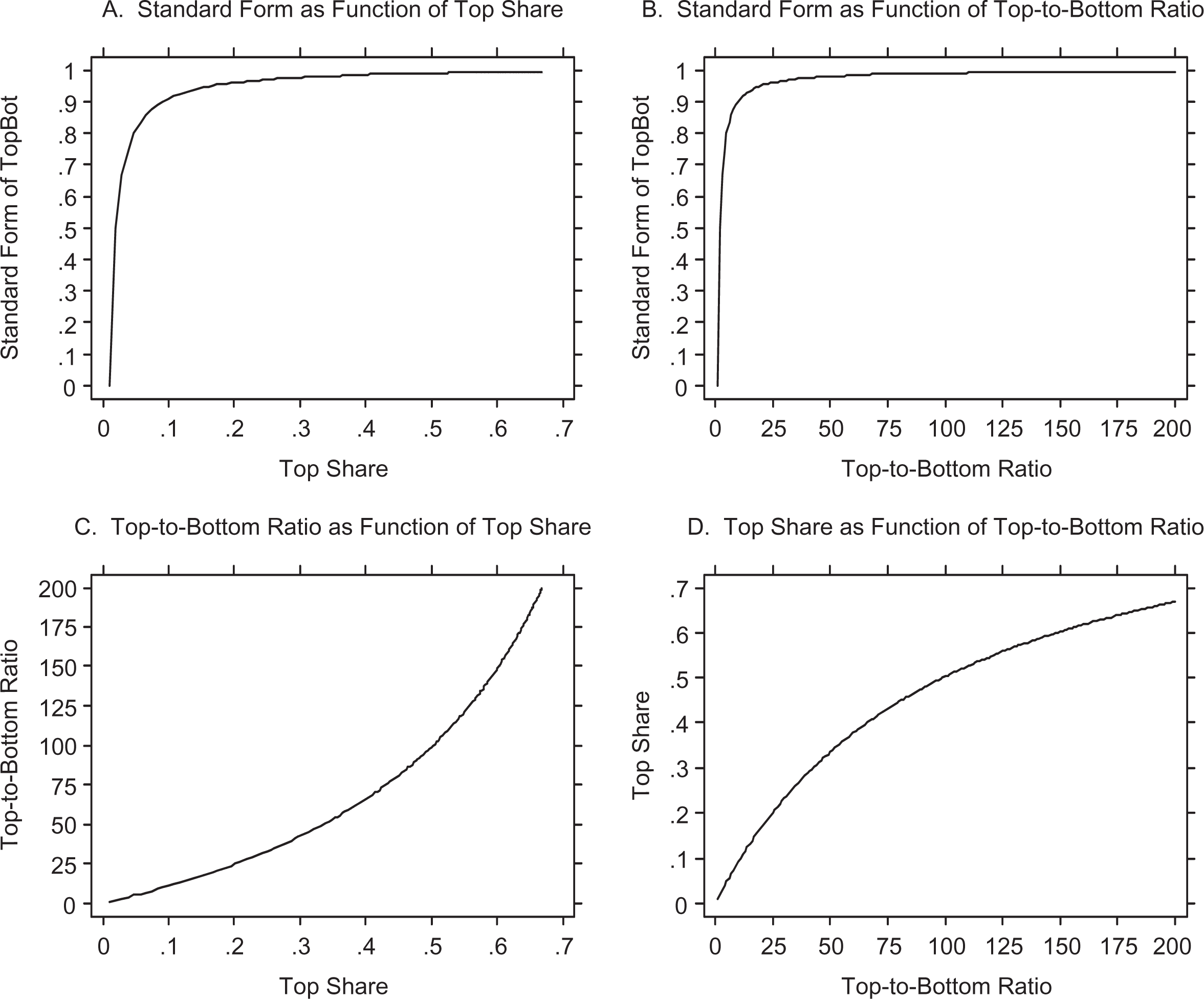
Relations between the ratios and shares of TopBot: top share, top-to-bottom ratio, standard form, for 99-1 percent split.

Thus, while it is good to have a standard form to include with the other manifestations of TopBot, for sheer rhetorical power, for intuitive appeal and ease of interpretation, this standard form cannot compete with the top share and the top-to-bottom ratio. The normalized ratio may be a good “dress blues” measure, to display when it is important to show that a member of the TopBot family satisfies the principle of normalization and to use for deepening understanding of inequality dynamics, but other work in the social science trenches—understanding determinants and consequences of inequality, for example, and policy formulation and assessment—will most likely be done by the top share and the top-to-bottom ratio.

The bluntness of the normalized ratio at the upper reaches of the income distribution underscores Cowell’s (2011:72-73) caution concerning the desirability of satisfying the principles of inequality measurement. There is little doubt that the top share and the top-to-bottom ratio outperform the normalized ratio on simplicity and interpretability.⁹

For contrast, Figure 1 also presents graphs of the top share and the top-to-bottom ratio as functions of each other (panels C and D). As shown, they are increasing and nonlinear, with the top-to-bottom ratio increasing at an increasing rate as the top share increases and the top share increasing at a decreasing rate as the top-to-bottom ratio increases. However, the nonlinear relations in panels C and D are mild compared to those in panels A and B.

Of course, as is well known, there are often multiple ways to construct a standard form, and different standard forms may behave differently. Look again at the basic relations in Table 1 and at the properties of the four ratios and shares at the end of the second section (“TopBot–Preliminaries”). The last of the four measures—the ratio of bottom average to top average µ^B/µ^T—provides the most direct route to a standard form, but not the only route. To illustrate, consider the top share S^T, which ranges from (1 − p) to one. A simple two-step procedure yields a standard form: first, subtract (1 − p), yielding a measure that ranges from zero to p; second, divide by p, yielding the desired standard form that sits on the unit interval, {[S^T/p] − [(1 − p)/p]}. Similarly, algebraic manipulation of the bottom share S^B yields the standard form [1 − (S^B/p)]. Visually, these two new standard forms appear to be linear functions of the top share and the bottom share, respectively. However, due to the exact relation between the top share and the bottom share (Table 1), they are merely different expressions of the same standard form, which can be written in terms of either the top share or the bottom share. Of course, it can be most useful to have alternative expressions for the same quantity, not only because one or the other may be more tractable across different situations but also because they reveal the “inner workings” of the quantity.¹⁰

For the reader’s convenience, we list the two standard forms and their three expressions, where SF denotes standard form, and for the second form, the suffixes B and T indicate whether the formula is based on the bottom share or the top share:

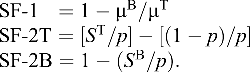
\begin{matrix} SF - 1 = 1 - μ^{B} / μ^{T} \\ SF - 2 T = [S^{T} / p] - [(1 - p) / p] \\ SF - 2 B = 1 - (S^{B} / p) . \end{matrix}

As discussed, SF-2T and SF-2B are equivalent and yield the same numerical outcomes. Note also that the second term in SF-2T is the ratio of the complementary percentages that lie at the heart of this work.

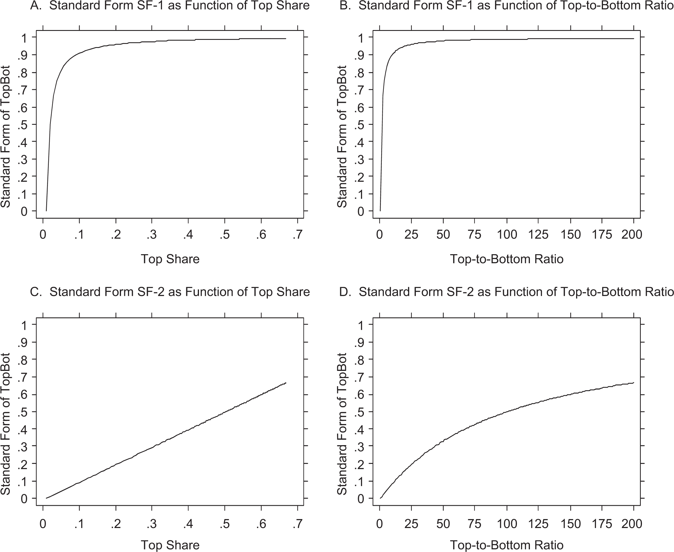
For a head-to-head contrast between the two standard forms, Figure 2 provides visualization, with panels A and B repeating the graphs in Figure 1 for the first standard form and panels C and D depicting the second standard form. Recall that the second standard form, in one of its guises, is a linear function of the top share. Thus, the graph of SF-2 on the top share (panel C) is an upward sloping straight line, exactly as expected, and the graph of SF-2 on the top-to-bottom ratio (panel D) resembles that of the top share on the top-to-bottom ratio (Figure 1, panel D)—nonlinear and increasing at a decreasing rate. The graph of SF-2 on the bottom share (not shown) is a downward sloping straight line. As for the contrast between the first and second standard forms, they seem a world apart, the first form dramatically nonlinear, the second adhering closely to the top share. Together, the two distinct standard forms of TopBot underscore the universality and versatility of the TopBot family.

Figure 2.

Two standard forms of TopBot, for 99-1 percent split.

TopBot and the correlations among its shares and ratios

To further understand the ratios and shares of TopBot, we examine their correlations in the constructed data set with 200 observations corresponding to top-to-bottom ratios ranging from 1 to 200. As expected from Figure 1 (panels C and D), the Pearson correlation of top share and top-to-bottom ratio is .961. However, the correlation of the standard form SF-1 and top share (panel A) is .518, and that of the standard form SF-1 and the top-to-bottom ratio (panel B) is .395. The nonlinearity is severe enough to substantially reduce the Pearson correlations among these measures, which are perfectly associated with each other. Of course, the Spearman rank-order correlations are exactly one.

The second standard form SF-2 (in either algebraic expression) is a linearly increasing function of the top share and a linearly decreasing function of the bottom share. Thus, its Pearson correlations are +1 with the top share and −1 with the bottom share. Its other correlations show the imprint of the top share. Its correlation with the top-to-bottom ratio is the same as that of the top share, .961, and its correlation with the bottom-to-top ratio is the negative of that between the top share and SF-1, −.518; and the correlation between SF-1 and SF-2 is .518.

The visualizations in Figure 1 also suggest that perhaps the classical concern with inequality measures’ differential sensitivity across regions of the income distribution can be fruitfully studied by mapping regions of bluntness and analyzing nonlinearities in the relations between inequality measures.

A New Link Between TopBot and the Gini Coefficient

From Atkinson (2007) and Alvaredo (2011), we know that top shares are mathematically related to the Gini coefficient. Atkinson (2007) observed that when the top subgroup is infinitesimal in numbers but with a finite share of total income, the Gini coefficient for the population can be approximated by an expression including the Gini coefficient for the bottom subgroup (everyone except the infinitesimally small top subgroup) and the top share. Alvaredo (2011) provided a formal proof for the expression and extended the result to the case where the top subgroup is not infinitesimal.

This section proposes a second connection between top shares and the Gini coefficient, further strengthening the Atkinson (2007) and Alvaredo (2011) results. As discussed above (first and second sections), top shares imply bottom shares, and bottom shares are none other than the Lorenz quantity. As is well known, (1) the Lorenz curve is the graph of the bottom share on the proportion in the bottom subgroup, namely, the graph of S^B on p, and (2) the Gini coefficient is tightly mathematically connected to the Lorenz curve. Thus, there must be a connection between top shares and the Gini coefficient.

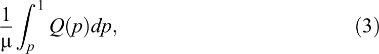
To understand this approach to linking top shares and the Gini coefficient, it is useful to begin with the connection between the Lorenz curve and the Gini coefficient. This connection can be expressed in several ways, including (1) twice the area between the Lorenz curve and the line of perfect equality (viz, the southwest to northeast [SW-NE] diagonal), (2) the ratio of the area between the Lorenz curve and the line of perfect equality to the total area below the diagonal (viz, one half), and (3) one minus twice the integral of the Lorenz curve (see, e.g., Gastwirth 1972:307; Kleiber and Kotz 2003:30; Stuart and Ord 1987:60-62). For example, the third way to express the connection begins with the bottom share, written in terms of the quantile function (QF), denoted Q(p):¹¹

\frac{1}{μ} \int_{0}^{p} Q (p) d p,

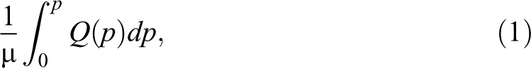
and proceeds to the Gini coefficient:

1 - \frac{2}{μ} \int_{0}^{1} \int_{0}^{p} Q (p) d p d p .

Informally, it may be said that the bottom share integrates to the Gini coefficient.¹²

Thus, the top share, via its intimate link to the bottom share (Table 1, panel B), is linked to the Gini coefficient, providing a second connection to supplement the Atkinson (2007) and Alvaredo (2011) results.

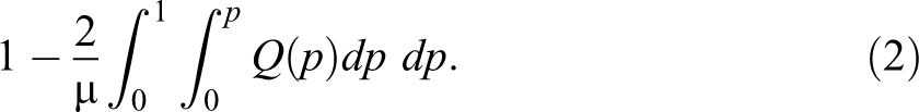
But a new natural question arises immediately: What is the direct relation between the top share and the Gini coefficient? Given the various expressions for the connection between the bottom share and the Gini coefficient, it is natural to expect a similar variety of expressions for the connection between the top share and the Gini coefficient. For example, following on the connection in expressions (1) and (2), it is straightforward to show that the Gini coefficient equals twice the integral of the top share minus one. Formally, starting with the expression for the top share:

\frac{1}{μ} \int_{p}^{1} Q (p) d p,

we can write the associated expression for the Gini coefficient:

[\frac{2}{μ} \int_{0}^{1} \int_{p}^{1} Q (p) d p d p] - 1.

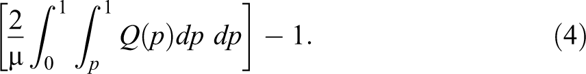
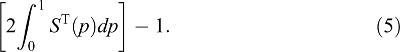
It can be readily verified that expression (2) equals expression (4), providing two parallel approaches to writing the connections between income shares and the Gini coefficient. That is, using bottom shares leads to expression (2), in which the Gini coefficient equals one minus twice the integral of the bottom share, and using top shares leads to expression (4), in which the Gini coefficient equals twice the integral of the top share minus one. Informally, it may be said that the bottom share and the top share each integrate to the Gini coefficient.

Denoting expression (3) for the top share by S^T (p), expression (4) for the Gini coefficient can be written more compactly:¹³

[2 \int_{0}^{1} S^{T} (p) d p] - 1.

The first and second ways highlighted above for expressing the link between the Lorenz curve and the Gini coefficient find similar parallels with top shares. To visualize the symmetries between the bottom share and the top share and their connections to the Gini coefficient, Figure 3 presents six plots. The first, in panel A, depicts the classic representation of the Lorenz curve. The plot shows the graph of the bottom share on the bottom proportion p, together with the equality line, the two forming a “basket.” The Gini coefficient is equal to twice the area in the basket, as in the first approach highlighted above to linking the Gini and the Lorenz curve (Kleiber and Kotz 2003:30). Thus, the deeper the basket, the greater the inequality. Moreover, by the second approach, the Gini equals the ratio of the area in the basket to the area below the diagonal (viz, one half).

Figure 3.

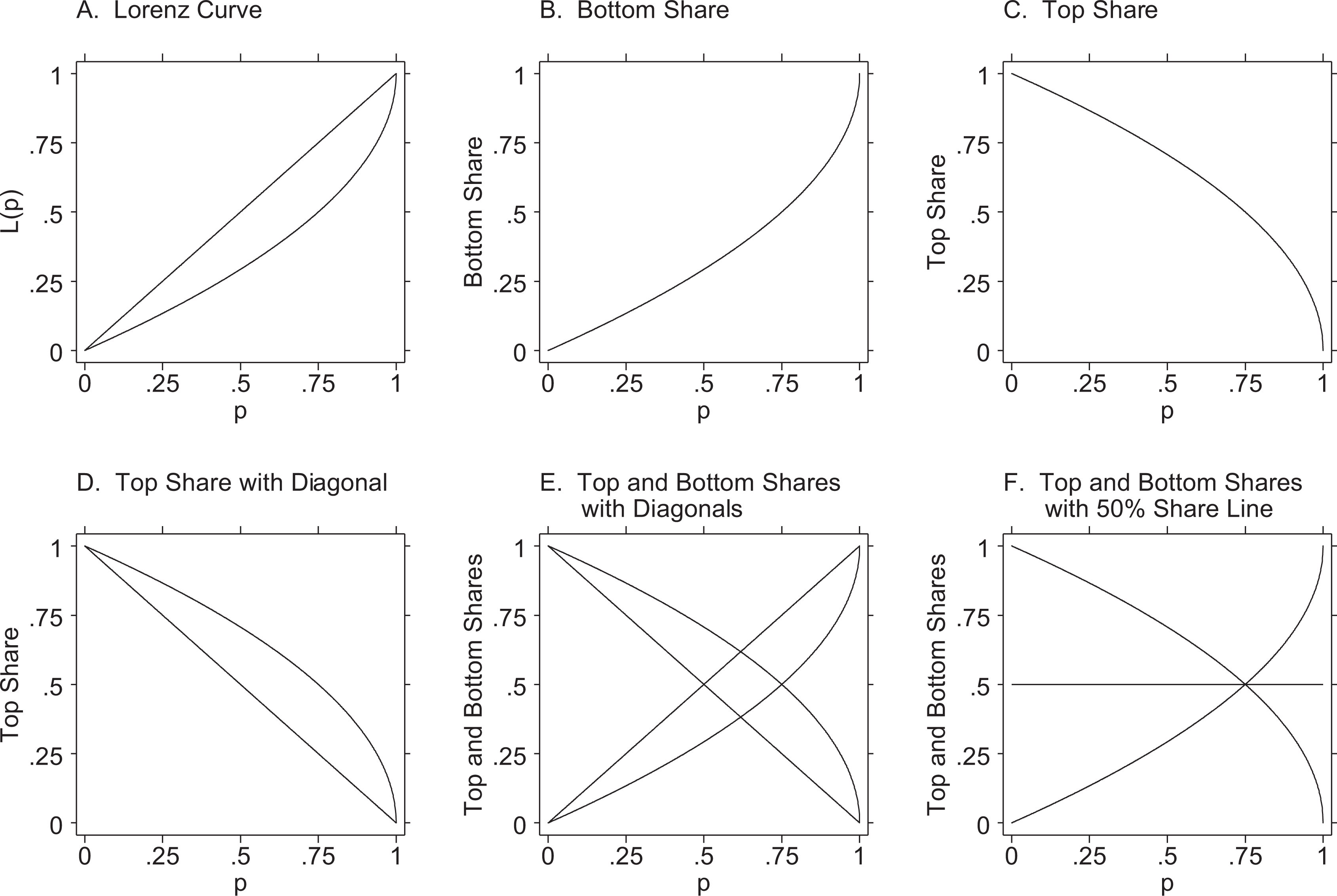
Visualizations of bottom and top shares.

Figure 3, panel B, depicts the same graph of the bottom share but omits the diagonal, highlighting the area under the curve—the relevant area for the link to the Gini coefficient in expression (2).

The third and fourth plots, in panels C and D, depict the top share in two versions analogous to the plots of the bottom share in panels A and B. In all the graphs, the top share is expressed as a function of the percent split p. For example, when p is .4, the top subgroup has 60 percent of the population and its share of income—the share of the top 60 percent—is over 75 percent (to the naked eye). Figure 3, panel C, shows the graph of the top share, alone on the grid (as the bottom share in panel B). The area under the top-share curve is the area linked to the Gini coefficient in expression (4).

Figure 3, panel D, adds a diagonal (the NW-SE diagonal that complements the diagonal in the Lorenz curve diagram in panel A), forming a picture of an inverted basket. The Gini coefficient is equal to twice the area in this inverted basket (analogous to the first way highlighted above for representing the link between the Lorenz curve and the Gini coefficient). Similarly, by the second way highlighted above, the Gini coefficient equals the ratio of the area in the basket in panel D to the area above the diagonal (viz, one half). It is illuminating to let the eye go from panel A to panel D and see the beautiful symmetry.

Finally, panels E and F of Figure 3 provide two views of both top shares and bottom shares together. Panel E combines the baskets in panels A and D. Panel F combines the sans-diagonals representations in panels B and C, showing that the graphs of the top and bottom shares are reflections of each other about the horizontal line at 50-percent shares. To the naked eye, it appears that the bottom 75 percent and the top 25 percent each hold half the income. Panel F indeed suggests an easy visualization of the intersection of top shares and bottom shares, answering the question at what percentage split do top and bottom subgroups each hold half the income.

The plots in Figure 3 also show vividly both that the top and bottom shares sum to one and that the integrals of the bottom share and top share sum to one. Panels E and F provide direct visualization of the relation between top and bottom shares (via vertical lines connecting the bottom-share and top-share curves at any point p). Panels B and C provide similarly direct visualization of the relation between the two integrals (given that the area under the bottom-share curve in panel B equals the area above the top-share curve in panel C).

The visualizations in Figure 3 lead to the inescapable conclusion that, paraphrasing the Broadway song by Irving Berlin, anything Lorenz curves can do top shares can do. Thus, top shares may have a rich parallel life of nonintersecting curves and curve dominance. And new angles of vision open new doors.

Further research will no doubt find more connections between TopBot and the Gini and possibly other classic measures of inequality as well.¹⁴

TopBot in Classical Probability Distributions

To further assess theoretically how TopBot tracks classic inequality measures like the Gini, Atkinson, and Theil measures, we investigate its behavior in three mathematically specified distributions whose properties are well known and which are widely used to model income distributions: the lognormal, Pareto, and power function (Johnson, Kotz, and Balakrishnan 1994, 1995; Kleiber and Kotz 2003). Together, this set includes combinations of bottom and top incomes useful for representing a variety of societies across space and time. The lognormal is defined for all positive values, the Pareto for all positive values larger than a specified number, and the power function for all positive values smaller than a specified number. Thus, the Pareto is appropriate for modeling distributions with a “safety net” and the power function for modeling distributions in times of scarcity.

All three are continuous univariate two-parameter distributions expressed in terms of the mean µ and a second parameter, denoted c, which Jasso and Kotz (2008), building on the literature pioneered by Pareto (1897) and more recent contributions such as Cowell (1977:95), Cramer (1971:51-58), Jasso (1987:96), and Kleiber and Kotz (2003:78, 115-18), suggest operates as a general inequality parameter governing all measures of overall inequality.¹⁵ Formulas for the major inequality measures in the three variates are well known (Cowell 1977, 2011; Kleiber and Kotz 2003), and Jasso and Kotz (2008) show that all are monotonic functions of the general inequality parameter c. Across the three variates, the general inequality parameter operates differently; it is a decreasing function of c for the Pareto and the power-function variates and an increasing function of c for the lognormal. To illustrate, the formula for the Gini coefficient in the Pareto is well known to be [1/(2c − 1)]. As the formula shows, inequality is solely a function of c; the first derivative, reported in Jasso and Kotz (2008:39), shows that the Gini is monotonic and, as expected, decreasing in c. The lognormal illustrates the opposite situation; in the lognormal, inequality is an increasing function of c, and the formulas for the inequality measures are increasing functions of c.¹⁶

Each of the three variates has a distinctive shape, as is well known. The lognormal has a mode toward the middle of the range and both a left tail going to zero and a long right tail. The Pareto has a mode at the nonzero minimum income and a long right tail. The power function has a mode whose location is at zero when c is less than one and at the maximum income when c is greater than one. A distinctive feature of the Pareto is that as inequality decreases, the minimum income increases. All three variates share the features that as inequality increases, the median gets smaller and the proportion below the mean increases.

The question now is whether the ratios and shares of TopBot are also monotonic functions of c in the three variates. If they are, then, in these variates, TopBot and the Gini, Atkinson, and Theil measures operate in similar ways and track each other.

Fortuitously, results already in the literature show that TopBot is a monotonic function of the general inequality parameter c in the three variates and thus joins the classical inequality measures as a set of measures that track each other and may be regarded as different manifestations of the same underlying inequality. The pertinent results are in work that addresses a different substantive question, namely, whether overall inequality is related to subgroup inequality, the latter defined as ratios and differences between averages in nonoverlapping subgroups formed by personal qualitative characteristics like race or gender. Of course, mathematically there is no difference between nonoverlapping subgroups of size p and (1 − p) and the bottom and top subgroups considered in the top share literature. And thus, the results obtained by Jasso and Kotz (2008) are directly applicable to TopBot.

Two results in particular apply directly. These pertain to the ratio of the bottom average to the top average (Jasso and Kotz 2008:44-49, esp. table 4 and figure 3) and to the bottom share (Jasso and Kotz 2008:49-52, esp. table 5 and figure 6), together with their first derivatives with respect to the general inequality parameter c. As already discussed above, these measures are related to the top-to-bottom ratio and to the top share—and, of course, to the standard forms of TopBot—and all are monotonic functions of c (Jasso and Kotz 2008).¹⁷

Thus, we conclude that TopBot is indeed an authentic measure of inequality. At least in the three variates under scrutiny, TopBot tracks the Gini, Atkinson, and Theil measures (as well as the coefficient of variation).

Table 2 reports the formulas for the bottom and top averages and top share of TopBot in the three variates. The subgroup averages are the building blocks for the ratios and directly related to the bottom and top shares (Table 1) and thus to the standard forms. As shown, all are functions of both the general inequality parameter c and the percent split p. Readers can use these formulas to model any combination of degree of inequality and percent split.

Table 2.

Bottom and Top Subgroup Means and Top Share in Probability Distributions.

Probability Distribution	Average in Bottom p µ^B	Average in Top (1 − p) µ^T	Top Share S^T
General	$\frac{1}{p} \int_{0}^{p} Q (p) d p$	$\frac{1}{1 - p} \int_{p}^{1} Q (p) d p$	$\frac{1}{μ} \int_{p}^{1} Q (p) d p$
Lognormal	$\frac{μ}{p} {F_{N} [Q_{N} (p) - c]}$	$\frac{μ}{1 - p} {1 - F_{N} [Q_{N} (p) - c]}$	$1 - F_{N} [Q_{N} (p) - c]$
Pareto	$\frac{μ [1 - {(1 - p)}^{(c - 1) / c}]}{p}$	$μ {(1 - p)}^{- 1 / c}$	${(1 - p)}^{(c - 1) / c}$
Power function	$μ p^{1 / c}$	$\frac{μ (1 - p^{(c + 1) / c})}{1 - p}$	$1 - p^{(c + 1) / c}$

Note: The bottom subgroup contains p proportion of the population and the top subgroup contains (1 − p) proportion. Accordingly, p denotes the percent split between the two subgroups, where 0 < p < 1. The average is denoted μ, and the superscripts B and T denote the bottom and top subgroups, respectively. General formulas are expressed in terms of the cumulative distribution function F(x) and the quantile function Q(α). The expressions $F_{N} (\cdot) and Q_{N} (\cdot)$ denote the cumulative distribution function and the quantile function, respectively, of the standard normal variate. Formulas for particular variates are expressed in terms of the mean μ and the general inequality parameter c, which in continuous univariate two-parameter distributions governs all measures of inequality. Inequality is a decreasing function of c for the Pareto and the power-function variates and an increasing function of c for the lognormal distribution.

The second and third sections (“TopBot–Preliminaries” and “TopBot and the Principles of Inequality Measurement”) noted that some of the shares and ratios of TopBot are nonlinearly related to each other. Now, considering together the formulas in the three variates for both the shares and ratios of TopBot and the classic inequality measures shows that, though they are all monotonic functions of the general inequality parameter, their relations with each other are mostly nonlinear. Exceptions include the relations (1) between the bottom and top shares, (2) between the bottom-to-top ratio and the standard form SF-1, (3) between SF-2 and either the top share or the bottom share, and (4) between the two Theil measures in the lognormal (which are identical). However, some of the nonlinearities appear mild. Nonetheless, these nonlinearities affect the Pearson correlations among the measures, though, of course, not the Spearman rank correlations.

TopBot in the Grand Scheme of Inequality Measures

TopBot as a measure of subgroup inequality

The fifth section (“TopBot in Classical Probability Distributions”) established that in at least a subset of probability distributions, the shares and ratios of TopBot and the classic measures of inequality are all monotonic functions of the general inequality parameter and thus track each other. But are there different types of inequality measures? And might TopBot and the classic measures be different types of inequality measures? If so, what type of inequality measure is TopBot?

The formulas provide a clue. The formulas for the classic inequality measures indicate that they are solely a function of the general inequality parameter c. For example, the formula for the Gini coefficient in the Pareto is [1/(2c − 1)]. In contrast, the formulas for TopBot indicate that they are a function not only of the general inequality parameter c but also of the percent split p, as shown in Table 2.

Returning to the results in Jasso and Kotz (2008), it is evident that all the measures of subgroup inequality examined in that work are functions not only of the general inequality parameter c but also, as would be expected, of the percent split p. Thus, it seems that there are indeed two types of inequality, overall inequality and subgroup inequality, and a measure’s formula indicates its type. The ratios and shares of TopBot are thus measures of subgroup inequality.

In a further twist, the formulas in Jasso and Kotz (2008) indicate that while ratios of subgroup averages are functions only of the general inequality parameter and the percent split, differences of subgroup averages are functions as well of the overall mean. Thus, there are two subtypes of measures of subgroup inequality, and TopBot is of the ratio subtype.

Methodologically, this work suggests a simple test for candidates for inequality measures. First, express the candidate measure in the form for mathematically specified distributions. Second, obtain the formulas for the candidate measure in two or three distributions, for example, the lognormal and Pareto. Third, inspect the formulas and their first partial derivatives. If they are monotonic functions of the general inequality parameter c, the candidate measure is a genuine measure of inequality. To establish what kind of measure the candidate measure is, given that it is a monotonic function of c, continue as follows. If the formulas are functions only of c, the candidate measure is a measure of overall inequality. If the formulas are functions of c and p, the candidate measure is a measure of subgroup inequality of the ratio subtype. If the formulas are functions of c, p, and µ, the candidate measure is a measure of subgroup inequality of the difference subtype.

Reconsidering TopBot and the Principle of Transfers

As discussed in the third section (“TopBot and the Principles of Inequality Measurement”), TopBot only weakly satisfies the principle of transfers. TopBot is blind to transfers within bottom and top subgroups. This would seem prima facie a serious disadvantage of TopBot. Obviously, a good measure of inequality should notice transfers from any part of the distribution to any other part. However, we now have two pieces of information that would seem to mitigate whatever disadvantage may accrue to TopBot based on weakly satisfying the principles of transfers. First, we now know, from the fourth section (“A New Link Between TopBot and the Gini Coefficient”), that TopBot is intimately linked to the Gini coefficient in exactly the same way that the Lorenz curve is linked to the Gini coefficient. Second, we now know, from the fifth section (“TopBot in Classical Probability Distributions”) and the subsection immediately above (“TopBot as a Measure of Subgroup Inequality”), that in an important class of probability distributions, TopBot varies together with classic measures which do satisfy the principle of transfers and is governed by the same general inequality parameter that governs them. Accordingly, TopBot would seem to be protected from disadvantages associated with its only weakly satisfying the principle of transfers by its double link to classic measures which do satisfy the principle of transfers—a universal link to the Gini coefficient and a link within an important class of probability distributions to all measures of inequality.

To explore the link within probability distributions and the protection it may provide, consider the case of a Pareto distribution with c = 2. In this case, the Gini coefficient equals 1/3, the Atkinson inequality equals approximately .176, the minimum income is half the mean, the proportion below the mean is .75, and the top 1 percent hold a top share of 10 percent. Suppose inequality increases, so that the general inequality parameter c = 1.5. Now the Gini coefficient equals .5, the Atkinson inequality equals approximately .351, the minimum income is one third the mean, the proportion below the mean is .808, and the top 1 percent hold a top share of 21.5 percent. Of course, transfers have occurred, and by algebraic manipulation of the QFs of the two distributions, it is straightforward to establish that transfers were made from the bottom 91.2 percent of the population to the top 8.8 percent. Thus, given that the two distributions are members of the Pareto family, information about any of these features—Gini coefficient, Atkinson inequality, minimum income, proportion below the mean, and top share—is sufficient to establish that transfers occurred and, further, exactly who lost income and who gained income.

More generally, if it is plausible that the underlying distributional family is stable, any of the above features (and others governed by the general inequality parameter) is sufficient to infer that transfers have occurred. In such situations then, information that the top share has increased is sufficient to infer that transfers have occurred.

Thus, the key to the protection provided by the link between measures of overall inequality and measures of subgroup inequality lies in the possibility that the distributional family is stable. If, however, the family is not stable, the link between overall and subgroup inequality is broken.

What are the clues to stability of distributional form? There are at least two. One is nonintersecting Lorenz curves (or, equivalently, nonintersecting top-share curves). A second is Spearman rank correlations of perfect unity.

Accordingly, the fact that TopBot, being a measure of subgroup inequality, only weakly satisfies the principle of transfers may be less of a disadvantage than at first appears, for (1) within distributional family, it is tightly linked to measures of overall inequality, which do satisfy the principle of transfers, and (2) regardless of distributional family, top shares are, like the Lorenz curve, tightly linked to the Gini coefficient, which does satisfy the principle of transfers.

Reconsidering TopBot and the Principle of Normalization

The third section (“TopBot and the Principles of Inequality Measurement”) showed the ease with which standard forms can be defined, so that TopBot satisfies the principle of normalization. But one of the standard forms, SF-1, does not share in the grace of the other shares and ratios of TopBot, particularly the top share and the top-to-bottom ratio. This appears to be a case where measures that do not satisfy a principle of inequality measurement outperform a measure that does, consistent with Cowell (2011:72-73). If SF-1 were TopBot’s only standard form, it would still provide a modicum of protection to the other shares and ratios, with which it is tightly linked, echoing the discussion above of the principle of transfers.

Fortunately, however, TopBot has another standard form, SF-2, which, as a linear function of both the top share and the bottom share, inherits their grace.

Insights for Empirics

As shown above, many of the shares and ratios of TopBot are nonlinearly related to each other, as are the classic measures of inequality. These nonlinearities suggest that the appropriate measure for analyzing relations among inequality measures is the Spearman rank correlation. In this section, we explore operation of TopBot and the classic inequality measures in the three variates already introduced—the lognormal, Pareto, and power function.

Table 3 uses the information in Table 2 to present 10 inequality scenarios in each of the three variates, all for the 99-1 percent split. The leftmost three columns report the linked top-to-bottom ratio, the top share, and the standard form SF-1. These are the same across the three variates. For example, algebraically, when the top-to-bottom ratio is 5, the top share is always .0481, and SF-1 is always .8. The 10 degrees of inequality displayed in Table 3—namely, 5–200 on the top-to-bottom ratio—were chosen to mirror the variation reported by Sommeiller et al. (2016, tables 1–3). For example, the top-to-bottom ratio among tax units in U.S. counties ranges from 5.1 in Wade Hampton County, Alaska, to 233 in Teton County, Wyoming. In metropolitan areas, the corresponding figures range from 5.9 in Junction City, Kansas, to 213 in Jackson, Wyoming-Idaho.

Table 3.

Three Expressions of TopBot for the Bottom 99 Percent and the Top 1 Percent—Ratio of the Top Average to the Bottom Average, Top Share, and Standard Form—With Features of the Implied Distribution in Three Variates.

Ratio μ^T/μ^B	Top Share S^T	1 − (μ^B/μ^T)	Features of Implied Distribution
Ratio μ^T/μ^B	Top Share S^T	1 − (μ^B/μ^T)	c	Minimum	Median	% Below Mean	Gini	Atkinson	Maximum
Lognormal
5	.0481	.800	.663	0	.803	.630	.361	.197	∞
15	.132	.933	1.207	0	.482	.727	.607	.518	∞
25	.202	.960	1.490	0	.329	.772	.708	.671	∞
50	.336	.980	1.902	0	.164	.829	.821	.836	∞
75	.431	.987	2.153	0	.0986	.859	.872	.901	∞
100	.503	.990	2.333	0	.0658	.878	.901	.934	∞
125	.558	.992	2.472	0	.0471	.892	.920	.953	∞
150	.602	.993	2.586	0	.0353	.902	.933	.965	∞
175	.639	.994	2.681	0	.0275	.910	.942	.973	∞
200	.669	.995	2.763	0	.0220	.916	.949	.978	∞
Pareto
5	.0481	.800	2.933	.659	.835	.706	.206	.0732	∞
15	.132	.933	1.787	.440	.649	.769	.388	.229	∞
25	.202	.960	1.533	.348	.547	.802	.484	.332	∞
50	.336	.980	1.311	.237	.402	.848	.617	.492	∞
75	.431	.987	1.224	.183	.322	.875	.691	.586	∞
100	.503	.990	1.176	.149	.269	.893	.740	.650	∞
125	.558	.992	1.145	.127	.232	.906	.775	.697	∞
150	.602	.993	1.124	.110	.204	.916	.802	.732	∞
175	.639	.994	1.108	.0974	.182	.924	.823	.760	∞
200	.669	.995	1.096	.0873	.164	.931	.839	.782	∞
Power function
5	.0481	.800	.256	0	.328	.665	.661	.901	4.902
15	.132	.933	.0767	0	.00167	.817	.867	→1	14.037
25	.202	.960	.0467	0	→0	.865	.915	→1	22.403
50	.336	.980	.0252	0	→0	.911	.952	→1	40.678
75	.431	.987	.0181	0	→0	.930	.965	→1	56.111
100	.503	.990	.0146	0	→0	.940	.972	→1	69.469
125	.558	.992	.0125	0	→0	.947	.976	→1	81.244
150	.602	.993	.0110	0	→0	.951	.978	→1	91.771
175	.639	.994	.00997	0	→0	.955	.980	→1	101.291
200	.669	.995	.00918	0	→0	.958	.982	→1	109.979

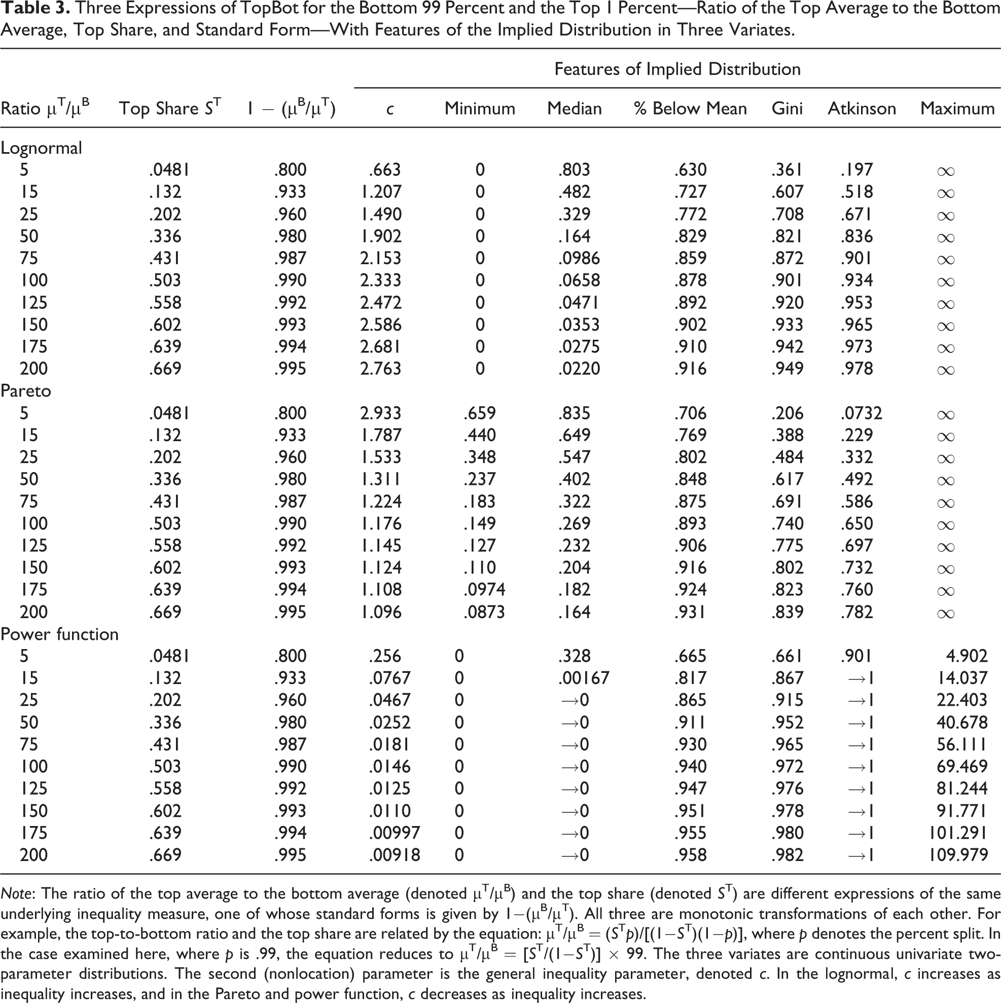
Note: The ratio of the top average to the bottom average (denoted μ^T/μ^B) and the top share (denoted S^T) are different expressions of the same underlying inequality measure, one of whose standard forms is given by 1−(μ^B/μ^T). All three are monotonic transformations of each other. For example, the top-to-bottom ratio and the top share are related by the equation: μ^T/μ^B = (S^Tp)/[(1−S^T)(1−p)], where p denotes the percent split. In the case examined here, where p is .99, the equation reduces to μ^T/μ^B = [S^T/(1−S^T)] × 99. The three variates are continuous univariate two-parameter distributions. The second (nonlocation) parameter is the general inequality parameter, denoted c. In the lognormal, c increases as inequality increases, and in the Pareto and power function, c decreases as inequality increases.

The fourth through tenth columns report features of the implied distributions, separately for the three variates. The first important feature is the general inequality parameter c. The formulas in Table 2 are used to solve for c from the top share or the standard form SF-1. In the lognormal (panel A), c increases with inequality, and thus it increases as the top-to-bottom ratio and the top share increase; the opposite occurs in the Pareto and power-function variates (panels B and C). Figures for the minimum, median, and maximum are expressed in terms of relative income (x/μ). Other columns report the proportion below the mean, the Gini coefficient, and the Atkinson measure defined as one minus the ratio of the geometric mean to the arithmetic mean (viz, when the inequality aversiveness parameter ε approaches 1).¹⁸

Notice that the correspondence between the TopBot measures and magnitudes of the Gini and Atkinson measures differs across variate. For example, when the top share is about 20 percent—approximately the level in the United States in 2013 (Sommeiller et al. 2016, table 10)—the Gini is .708 in the lognormal, .484 in the Pareto, and .915 in the power function. More broadly, as the top-to-bottom ratio moves from 5 to 200 (Table 2, leftmost column), the Gini inhabits a distinctive region of the unit interval in each of the three variates—.361 to .949 in the lognormal, .206 to .839 in the Pareto, and .661 to .982 in the power function. Within variate, the correlations between the Gini and the measures of TopBot will be fairly high, and the Spearman correlations will be one.

Now imagine a disjuncture—in a time series, say, a country’s income distribution changes shape; or in a set of countries, new countries are incorporated, whose income distributions differ in shape from those in the original set. Both the Pearson and the Spearman correlations will weaken substantially. To illustrate, suppose a country’s income distribution is approximated by a lognormal. As the top-to-bottom ratio increases from 5 to 75, the Gini goes from .361 to .872 (Table 3, panel A), but a shift to the Pareto form will move the Gini from .872 down to .74, when the top-to-bottom ratio reaches 100; even when the top-to-bottom ratio is 200, the Gini will only be .839—less than the .872 in the lognormal era when the top-to-bottom ratio was 75. And similarly for the Atkinson measure, as can be easily verified from Table 3.

This means that weakening relations between the top share and the Gini, such as discussed in Morelli et al. (2015), may signal differences or shifts in the distributional shapes of the income distributions under study. Such differences and shifts in distributional shape are themselves important signals of income dynamics and merit further empirical study.

More broadly, any two inequality measures will have, within distributional form, high Pearson correlations and perfect Spearman correlations. Accordingly, weakening relations between any two inequality measures—say the Gini and Atkinson—signal differences or shifts in distributional forms, as can also be verified from Table 3. Thus, examining the relations between inequality measures in income distributions is not only methodologically useful but also sheds light on underlying income dynamics.

To further explore this activity, we constructed two parallel data sets based on the constructed data just described. Each of the data sets is a subset of the original constructed data, the subset defined by top-to-bottom ratios that range from 13 to 45. These magnitudes form the endpoints of the actual ratios observed by Sommeiller et al. (2016) for the 50 states in the United States. As discussed above, the lowest inequality state is Alaska with a top-to-bottom ratio of 13.2, and the highest inequality state is New York with a ratio of 45.4 (Sommeiller et al. 2016, table 10). One of the two data sets was designated as a lognormal, the other as a Pareto, and the observations include all the corresponding measures from panels A and B of Table 3. We also included the two Theil measures and, in the lognormal data set, the coefficient of variation.¹⁹

We then obtained the Pearson and Spearman correlation matrices, separately within each data set. As expected, within each data set, the Pearson matrices largely departed from unity, except for pairs known to be linearly related (such as the top share and the bottom share or, in the lognormal, the two Theil measures). The Spearman correlation matrix showed a perfect set of ones.

Then, we experimented with replacing observations in each data set with observations from the other data set corresponding to the same top-to-bottom ratio. For example, we would replace the observation for the top-to-bottom ratio of 22 in the lognormal with the observation with the same top-to-bottom ratio in the Pareto and so on. In these experiments, the Spearman correlation matrices departed from perfect unity.

The challenge for empirical work is to detect subsets of distributions with Spearman correlation matrices of perfect unity and to analyze how the correlations weaken when distributions from one subset are mixed with distributions from another subset. This topic warrants further research.

Concluding Note

Newly precise evidence of the trajectory of top incomes in the United States and around the world relies on shares and ratios, prompting new inquiry into their properties as inequality measures. Current theoretical and empirical evidence, based on the pioneering work of Atkinson (2007) and Leigh (2007), and extended and strengthened by Alvaredo (2011), Morelli et al. (2015), and Roine and Waldenström (2015), shows that top shares satisfy four principles of inequality measurement (albeit one of them weakly), suggests a mathematical link between top shares and the Gini coefficient, and documents empirical links extending as well to the Atkinson measure. The work reported in this article strengthens that evidence, making several contributions: First, it formalizes the shares and ratios, showing that as monotonic transformations of each other, they are different manifestations of a single inequality measure, here called TopBot. Second, it shows that TopBot satisfies three other principles of measurement, proposing two standard forms of TopBot that satisfy the principle of normalization—(1) one minus the bottom-to-top ratio and (2) a form which can be expressed as a linear function of either the top share or the bottom share. Third, it presents a second algebraic link between TopBot and the Gini coefficient, showing that all the useful results accumulated for the Lorenz curve pertain as well to top-share curves. Fourth, it investigates TopBot in mathematically specified probability distributions, showing that TopBot is monotonically related to classical measures such as the Gini, Atkinson, and Theil measures and the coefficient of variation. Thus, TopBot appears to be a genuine inequality measure, specifically a measure of subgroup inequality with a double link to classic measures—a universal link to the Gini coefficient and a link within an important class of probability distributions to all inequality measures. Moreover, TopBot is further distinguished by its ease of calculation and ease of interpretation, making it an appealing People’s measure of inequality.

This work also provided new insights, for example, that, given nonlinearities in the (monotonic) relations among inequality measures, Spearman correlations are more appropriate than Pearson correlations and that weakening of correlations among inequality measures (such as between TopBot and the Gini or between the Gini and Atkinson measures) signals differences and shifts in distributional form, suggesting that the study of correlations among inequality measures is not only methodologically useful but also sheds light on income dynamics.

Of course, much further work remains to be done—finding further algebraic links between the shares/ratios of TopBot and classic inequality measures, finding further relations between TopBot and classical inequality measures in mathematically specified probability distributions, including distribution-independent relations, and broadening empirical work to include both a larger set of income distributions and a larger set of inequality measures.

At this point, all the evidence suggests that TopBot is an authentic measure of inequality, and, with its complement of top shares, top-to-bottom ratios, and standard forms, a useful measure of inequality.

Footnotes

Acknowledgments

Earlier versions of this article were presented at the MidYear Meeting of the ASA Methodology Section, Chicago, IL, April 2017; at the 10th Conference of the International Network of Analytical Sociologists (INAS), University of Oslo, Norway, June 2017; at DIW Berlin, July 2017; at the Seventh Meeting of the Society for the Study of Economic Inequality (ECINEQ), City University of New York, July 2017; and at the Joint Statistical Meetings, Baltimore, MD, August 2017 and at the XIX World Congress of the International Sociological Association (ISA), RC28, Toronto, Canada, July 2018. I am grateful to conference participants and to Charlotte Bartels, Jun Kobayashi, Arnout van der Rijt, Jürgen Schupp, Gert G. Wagner, Yu Xie, the anonymous referees, and the Editor for valuable comments and suggestions. I also gratefully acknowledge the intellectual and financial support of New York University. Finally, this paper is dedicated to Samuel Kotz (1930–2010); had he lived, he would have loved to work on it.

Declaration of Conflicting Interests

The author(s) declared no potential conflicts of interest with respect to the research, authorship, and/or publication of this article.

Funding

The author(s) received no financial support for the research, authorship, and/or publication of this article.

Notes

References

Alvaredo

Facundo

. 2011. “A Note on the Relationship Between Top Income Shares and the Gini Coefficient.” Economics Letters 110:274–77.

Alvaredo

Facundo

Atkinson

Anthony B.

Piketty

Thomas

Saez

Emmanuel

Zucman

Gabriel

. 2011–2017. The World Wealth and Income Database. Retrieved from http://www.wid.world/, 8 December 2016. World Inequality Database, retrieved from http://www.wid.world/, 25 March 2018.

Atkinson

Anthony B.

2007. “Measuring Top Incomes: Methodological Issues.” Pp. 18–42 in Top Incomes Over the Twentieth Century: A Contrast Between Continental European and English-Speaking Countries, edited by Atkinson

Anthony B.

Piketty

Thomas

. Oxford, England: Oxford.

Atkinson

Anthony B.

Piketty

Thomas

Saez

Emmanuel

. 2011. “Top Incomes in the Long Run of History.” Journal of Economic Literature 49:3–71.

Cowell

Frank A.

1977. Measuring Inequality: Techniques for the Social Sciences. New York: Wiley.

Cowell

Frank A.

2011. Measuring Inequality, 3rd ed. Oxford, England: Oxford University.

Cramer

Jan S.

1971. Empirical Econometrics. New York: Elsevier North-Holland.

Dagum

Camilo

. 1983. “Income Inequality Measures.” Pp. 34–40 in Encyclopedia of Statistical Sciences. Vol. 4, edited by Kotz

Samuel

Johnson

Norman L.

Read

Campbell B.

. New York: Wiley.

Dalton

Hugh

. 1920. “The Measurement of the Inequality of Incomes.” Economic Journal 30:348–61.

10.

Feenberg

Daniel R.

Poterba

James M.

. 1993. “Income Inequality and the Incomes of Very High-income Taxpayers: Evidence from Tax Returns.” Tax Policy and the Economy 7:145–77.

11.

Gastwirth

Joseph L.

1971. “A General Definition of the Lorenz Curve.” Econometrica 39:1037–39.

12.

Gastwirth

Joseph L.

1972. “The Estimation of the Lorenz Curve and Gini Index.” The Review of Economics and Statistics 54:306–16.

13.

Gastwirth

Joseph L.

2014. “Median-Based Measures of Inequality: Reassessing the Increase in Income Inequality in the U.S. and Sweden.” Statistical Journal of the IAOS (International Association for Official Statistics) 30:311–20.

14.

Gini

Corrado

. 1914. “Sulla Missura della Concentrazione e della Variabilità dei Caratteri.” Atti del Reale Istituto Veneto di Scienze, Lettere ed Arti 73:1203–48.

15.

Gould-Wartofsky

Michael A.

2015. The Occupiers: The Making of the 99 Percent Movement. New York: Oxford.

16.

Jasso

Guillermina

. 1987. “Choosing a Good: Models Based on the Theory of the Distributive-Justice Force.” Advances in Group Processes: Theory and Research 4:67–108.

17.

Jasso

Guillermina

Kotz

Samuel

. 2008. “Two Types of Inequality: Inequality Between Persons and Inequality Between Subgroups.” Sociological Methods and Research 37:31–74.

18.

Johnson

Norman L.

Kotz

Samuel

Balakrishnan

. [1994] 1995. Continuous Univariate Distributions. Vol. 1, 2nd ed. New York: Wiley.

19.

Keister

Lisa A.

Lee

Hang Young

. 2014. “The One Percent: Top Incomes and Wealth in Sociological Research.” Social Currents 1:13–24.

20.

Kleiber

Christian

Kotz

Samuel

. 2003. Statistical Size Distributions in Economics and Actuarial Sciences. Hoboken, NJ: Wiley.

21.

Kuznets

Simon

. 1953. Shares of Upper Income Groups in Income and Savings. Cambridge, MA: National Bureau of Economic Research.

22.

Lampman

Robert

. 1962. The Share of Top Wealth-Holders in National Wealth, 1922-1956. Princeton, NJ: Princeton.

23.

Leigh

Andrew

. 2007. “How Closely Do Top Income Shares Track Other Measures of Inequality?” Economic Journal 117:F619–33.

24.

Morelli

Salvatore

Smeeding

Timothy

Thompson

Jeffrey

. 2015. “Post-1970 Trends in Within-Country Inequality and Poverty: Rich and Middle-Income Countries.” Pp. 593–696 in Handbook of Income Distribution. Vol. 2A, edited by Atkinson

Anthony B.

Bourguignon

François

. London, England: Elsevier.

25.

Pareto

Vilfredo

. 1897. Cours d’Economie Politique. Lausanne, Switzerland: Rouge.

26.

Pietra

Gaetano

. 1915. “Delle Relazioni fra Indici de Variabilità, Note I e II.” Atti del Reale Istituto Veneto di Scienze, Lettere ed Arti 74:775–804.

27.

Pigou

Arthur Cecil

. 1912. Wealth and Welfare. London, England: Macmillan.

28.

Piketty

Thomas

. 2001. Les Hauts Revenus en France au XXe Siècle: Inégalités et Redistributions, 1901-1998. Paris, France: Grasset.

29.

Piketty

Thomas

. 2003. “Income Inequality in France, 1901-1988.” Journal of Political Economy 111:1004–42.

30.

Piketty

Thomas

Saez

Emmanuel

. 2003. “Income Inequality in the United States, 1913-2002.” Quarterly Journal of Economics 118:1–39.

31.

Roine

Jesper

Waldenström

Daniel

. 2015. “Long-Run Trends in the Distribution of Income and Wealth.” Pp. 469–592 in Handbook of Income Distribution. Vol. 2A, edited by Atkinson

Anthony B.

Bourguignon

François

. London, England: Elsevier.

32.

Schutz

Robert R.

1951. “On the Measurement of Income Inequality.” American Economic Review 41:107–22.

33.

Sommeiller

Estelle

Price

Mark

Wazeter

Ellis

. 2016. Income Inequality in the U.S. by State, Metropolitan Area, and County. Washington, DC: Economic Policy Institute. Retrieved from http://www.epi.org/107100, 28 August 2016.

34.

Stiglitz

Joseph E.

2011. “Of the 1%, by the 1%, for the 1%.” Vanity Fair 53(5):126.

35.

Stuart

Alan

Ord

J. Keith

. 1987. Kendall’s Advanced Theory of Statistics, Distribution Theory. Vol. 1, 5th ed. Originally by Sir Maurice Kendall. New York: Oxford University Press.