A Note on a Reformulation of the KHB Method

Abstract

The Karlson–Holm–Breen (KHB) method has rapidly become popular as a way of separating the impact of confounding from rescaling when comparing conditional and unconditional parameter estimates in nonlinear probability models such as the logit and probit. In this note, we show that the same estimates can be obtained in a somewhat different way to that advanced by Karlson, Holm, and Breen in their original article and implemented in the user-written Stata command khb. While the KHB method and this revised KHB method both work by holding constant the residual variance of the model, the revised method makes comparisons across multiple nested models easier than the original method.

Keywords

nonlinear probability models logit model probit model nested model comparisons KHB method

Sociologist and other social scientist routinely compare coefficients across same-sample nested models. For instance, when sociologists want to investigate how much of the association between a variable of interest, X, and an outcome, Y, is mediated through a third variable, Z, they often first fit a model with Y as the dependent variable and X as the predictor. Then, they fit another model that adds Z as a control variable. The coefficient for X from this model is compared with the corresponding coefficient from the first model. The difference between the two is then taken as a measure of how far the relationship between X and Y is mediated by Z.

If the models used are linear (estimated by, e.g., ordinary least squares [OLS]), this procedure is unproblematic, but this is not so for nonlinear models such as the logit, probit, multinomial logit, or ordered logit, which would often be used if the outcome, Y, were categorical or ordinal. Because nonlinear models are noncollapsible over confounders (or mediators), the change in the coefficient of the independent variable of interest is not solely driven by mediating or confounding by the added variables; part of the change is due to change in the residual variance of the models. The more variables that are included in a nonlinear probability model, the smaller the residual variance, and because the variance and mean are not separately identified in these models, change in the residual variance also affects the coefficient estimates. One consequence of this is that, even if a variable unrelated to X is added to the model, the coefficient of X will change.¹

Several methods have been suggested to separate this so-called rescaling effect from the true degree of confounding or mediation. They include Y-standardization, average marginal effects, and, more recently, the Karlson–Holm–Breen (KHB) method. The KHB method compares the regression coefficients for the variable of interest X from two models. One includes X and the mediators/confounders, Z (which may be a single variable or a vector), and one includes X and a residualized version of Z. The Z variables are residualized with respect to X. Both models have the same predictive power and hence the same residual variance, but the residualized Z are uncorrelated with X, and so a comparison of coefficients of the independent variable of interest across these models reveals the true impact of mediation/confounding on the coefficient for X.

In this article, we present a simple method to obtain exactly the same measure of confounding/mediation, using the latent index (i.e., the estimated linear predictor) from a nonlinear probability model. We show that this approach allows the researcher to infer the amount of mediation/confounding through simple linear regression analyses. We illustrate it with an example using the ordered logit model.

Method

We begin by defining the following latent linear regression models:

Y^{*} = β_{0} + β_{1} X + β_{2} Z + ∊ (full model),

Y^{*} = γ_{0} + γ_{1} X + ν (reduced model),

where $Y^{*}$ is a continuous, but unobserved, latent dependent variable; X is the independent variable of interest; Z is a mediator or confounder; $∊$ is an error term assumed to be independent of X and Z; and $ν$ is an error term assumed independent of X. Z may be a single variable or a vector of variables.

We observe the binary indicator, Y, defined in terms of the unobserved $Y^{*}$ by

\begin{array}{l} Y = 1 if Y^{*} > τ, \\ Y = 0 if Y^{*} \leq τ, \end{array}

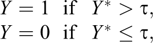
with $τ$ being an unknown threshold.

The nonlinear regressions corresponding to the latent linear models are

h (p r (Y = 1)) = b_{0} + b_{1} X + b_{2} Z,

h (p r (Y = 1)) = c_{0} + c_{1} X,

where $h (...)$ is a nonlinear transformation such as the logit or probit. We know that the relationship between the coefficients of the nonlinear regression model, equation (2a), and the latent variable model, equation (1a), is $b_{j} = \frac{β_{j}}{s}, j = 1, 2$ , where s is a scale factor that allows the variance of the error term in equation (1a) to differ from that of an assumed standard distribution such as the standard logistic or standard normal. The same holds for the relationship between the coefficients in equations (2b) and (1b), albeit with a different scale factor (since this reflects the residual or unexplained variance of the model).

The KHB method works by residualizing the mediator/confounder, Z, by regressing it on X using OLS, and then another nonlinear model is estimated:

h (p r (Y = 1)) = a_{0} + a_{1} X + a_{2} \tilde{Z},

where $\tilde{Z}$ is the residualized Z. This corresponds to an underlying latent model:

Y^{*} = α_{0} + α_{1} X + α_{2} \tilde{Z} + u,

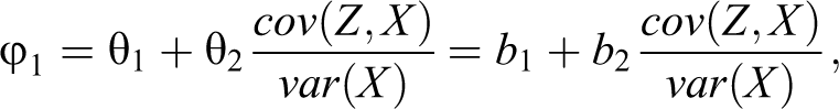
where u is an error term assumed to be independent of X and Z. Karlson, Holm, and Breen (2012) show that $∊$ = u (and thus their variances and the implied scale factors are the same) and that $α_{1} = γ_{1}$ . It then follows that the KHB estimator, $\frac{b_{1}}{a_{1}}$ is equal to $\frac{β_{1}}{γ_{1}}$ , that is, the ratio of the conditional (partial) to the unconditional (gross) coefficient of X in the underlying latent model.

The revised method presented here recovers the same ratio but in an easier way. Define V as the linear predictor (latent index) from equation (2a), that is,

V = h^{- 1} (p r (Y = 1)) = b_{0} + b_{1} X + b_{2} Z .

Next, we fit two OLS models, using V as the dependent variable:

V = θ_{0} + θ_{1} X + θ_{2} Z,

V = φ_{0} + φ_{1} X + ω .

Equation (6a) has no error term because it is saturated: It fits the data perfectly.

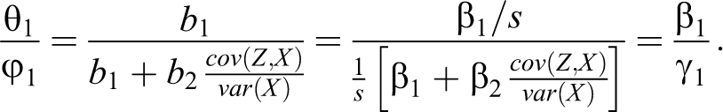
Karlson et al. (2012) proved that the KHB method recovers the ratio $\frac{β_{1}}{γ_{1}}$ . From equations (1a) and (1b), this ratio is equal to:

\frac{β_{1}}{γ_{1}} = \frac{β_{1}}{β_{1} + β_{2} c o v (Z, X) / v a r (X)} .

Thus, we need to show that the revised method, using equations (6a) and (6b), recovers the same ratio: That is, we need to show that $\frac{θ_{1}}{φ_{1}} = \frac{β_{1}}{γ_{1}}$ .

For all coefficients, we know that $θ_{j} = b_{j}$ holds, that is, the coefficients from the linear model fitted to the latent index are the same as the coefficients that generated the latent index. Then,

φ_{1} = θ_{1} + θ_{2} \frac{c o v (Z, X)}{v a r (X)} = b_{1} + b_{2} \frac{c o v (Z, X)}{v a r (X)},

and this yields

\frac{θ_{1}}{φ_{1}} = \frac{b_{1}}{b_{1} + b_{2} \frac{c o v (Z, X)}{v a r (X)}} = \frac{β_{1} / s}{\frac{1}{s} [β_{1} + β_{2} \frac{c o v (Z, X)}{v a r (X)}]} = \frac{β_{1}}{γ_{1}} .

This method returns exactly the same ratio estimates of confounding or mediation as the KHB method, and these are equal to the true ratio in the underlying latent variable model in equations (1a) and (1b).

Comparing the Revised Method With the Original KHB

The method proposed here requires the following steps:

fit the full model, including X and all other predictors of Y, as a logit or other nonlinear probability model;

save the latent index from this model; and

taking the latent index as the dependent variable, use OLS models (with and without the mediators/confounders), to estimate the extent of mediation or confounding.

The steps for the original KHB method are:

regress the confounder on the independent variable of interest,

obtain the predicted values from this regression,

fit the full model, and

fit the reduced model, controlling for the predicted values.

At first sight, it may seem that both methods are equally convenient, but suppose we wanted to introduce meditating or confounding variables sequentially (i.e., through successive models, starting with a model including Z ₁, followed by a model including Z ₁ and Z ₂, and so on) to see where the coefficient of X changed most. In this case, the method presented here would be more convenient because it would not require any extra steps other than an additional OLS regression including both Z ₁ and Z ₂. Using the KHB method, however, we would need to residualize both of these, using separate regressions. As the number of mediators or confounders whose impact we want to assess increases, so does the computational advantage of the new method.

Standard Errors

Karlson et al. (2012:295-96) developed a Z-test for whether the conditional and unconditional effects of X are equal (this is labeled Z_c ). It is a test of whether the coefficient of X is changed by true confounding or mediation, net of the effect of rescaling. In our notation, this test would be written as:

Z_{C} = \frac{a_{1} - b_{1}}{s . e . (a_{1} - b_{1})} .

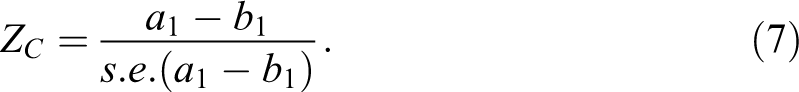
This is equivalent to a test of the significance of the product $b_{2} ψ_{1}$ , where $ψ_{1}$ is the estimated coefficient from the equation used to residualize Z:

Z = ψ_{0} + ψ_{1} X + ω .

Karlson et al. (2012) use the delta method to derive the standard error of $b_{2} ψ_{1}$ and thus the Z-test of the significance of the difference between the conditional and unconditional coefficients of X measured on the scale of the full model.

As an alternative, the bootstrap is a fast and convenient way of obtaining standard errors (the analytical standard errors based on the delta method can be cumbersome to calculate without specialized software).² Another advantage of using the bootstrap for estimating standard errors is that one can easily compute standard errors of differences of coefficients, that is, of indirect effects, or of ratios of coefficients such as the percentage mediated. In this case, we would often care about our estimate of the ratio $\frac{θ_{1}}{φ_{1}}$ . To test whether it differed significantly from 1, we would need to calculate its standard error, and this may be awkward, not only because it is a ratio of two estimated parameters but also because the method presented here uses another estimated quantity—namely V—in its derivation. Because V is estimated from the data, the uncertainty in that estimate must also be taken into account in estimating the standard error of $\frac{θ_{1}}{φ_{1}}$ . Both these issues are easily dealt with using the bootstrap, but we need to bootstrap not just the OLS regressions used to estimate $θ_{1}$ and $ϕ_{1}$ but also the nonlinear probability model used to generate V. So the bootstrap steps are as follows: estimate equation (2a), use this to calculate V (equation [5]), fit equations (6a) and (6b), and save the estimated ratio $\frac{θ_{1}}{φ_{1}}$ . The same sequence applies to get the bootstrap standard errors for any other quantities of interest.³

Example: Parental Income and Support for Redistribution

To illustrate how our method works, we examine potential mediators of the association between parental income and individuals’ stated support for redistribution in the United States using the 1987, 1993, 1994, 2008, and 2010 waves of the General Social Survey. The final sample after listwise deletion is 3,603.

The outcome variable is the respondents’ response to a question about whether the government should reduce income differentials and has five ordered response categories: strongly disagree, disagree, neither, agree, and strongly agree. The main predictor variable is the respondent’s parents’ income when the respondent was 16 years old. We recode this variable into three levels: below average, at average, and above average. As mediators we include socioeconomic and sociodemographic characteristics of the respondent: the respondent’s income grouped into 12 income bins (which we use as a continuous covariate), the respondent’s years of schooling, the respondent’s occupational prestige score (2010 scoring on a 100-point scale), the marital status of the respondent (married, widowed, divorced, separated, and never married), and the respondent’s region of residence (New England, Middle Atlantic, East North Central, West North Central, South Atlantic, East South Central, West South Central, Mountain, and Pacific). In addition to these variables, we control all models for survey year fixed effects and the respondent’s age to balance the sample on these characteristics.

Table 1 shows the estimated association, using ordered logit models, between parental income and a respondent’s support for government action to reduce income differentials. The gross or unmediated association in model 1 (M1) suggests that respondents born to affluent parents less often support redistribution (as defined here). Introducing respondent characteristics as mediators leads to a decline in the effect of parental income across the models, particularly across the first three. For example, the coefficient for above-average parental income declines by 24.7 percent from M1 (−.673) to model M3 (−.507).

Table 1.

Ordered Logit Models Regressing Support for Redistribution on Parental and Respondent Characteristics.

	Model 1	Model 2	Model 3	Model 4	Model 5
Parental income
Below average (reference)
At average	−0.378 (0.069)	−0.353 (0.070)	−0.322 (0.070)	−0.320 (0.070)	−0.321 (0.070)
Above average	−0.673 (0.088)	−0.618 (0.088)	−0.507 (0.090)	−0.506 (0.090)	−0.515 (0.090)
Respondent characteristics		−0.0784	−0.0642	−0.0601	−0.0580
Income		−0.0784	−0.0642	−0.0601	−0.0580
Years of schooling			−0.0661	−0.0559	−0.0575
Occupational prestige				−0.00503	−0.00385
Marital status controlled	No	No	No	No	Yes
Region controlled	No	No	No	No	Yes
Thresholds
Threshold 1	−2.985	−3.532	−4.305	−4.334	−4.079
Threshold 2	−1.320	−1.848	−2.607	−2.636	−2.369
Threshold 3	−0.414	−0.929	−1.684	−1.712	−1.439
Threshold 4	1.457	0.960	0.208	0.181	0.464

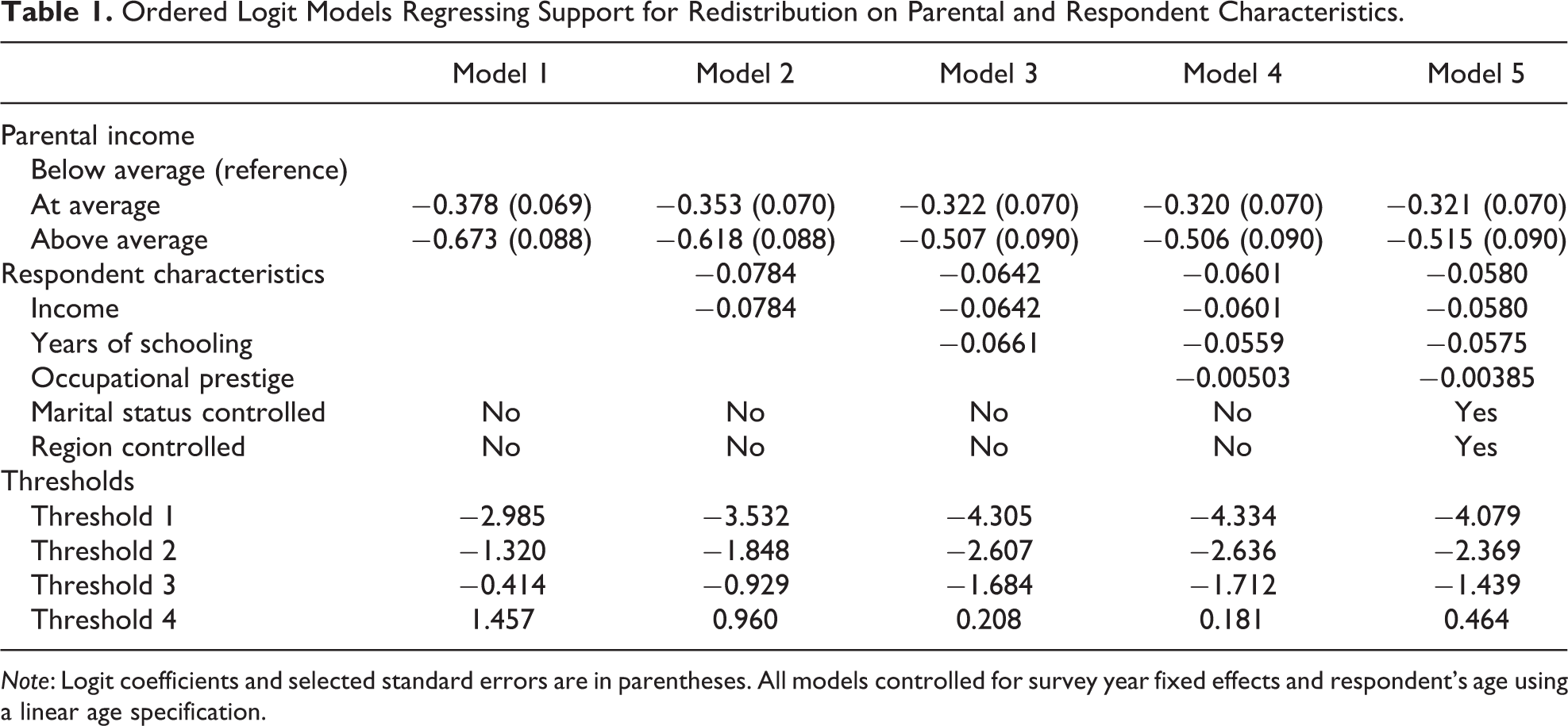
Note: Logit coefficients and selected standard errors are in parentheses. All models controlled for survey year fixed effects and respondent’s age using a linear age specification.

Rescaling may influence comparisons of the effect of parental income across these same-sample nested models. Therefore, in Table 2, we report the corresponding estimates using the revised KHB approach detailed in this article. It appears that, in fact, changes in the coefficients are not substantively driven by rescaling: The rescaling effect is negligible, as can be seen by comparing the gross association in the first columns in Tables 1 and 2. For example, the coefficient for above-average parental income declines by 26.2 percent from M1 (−.693) to M3 (−.511). This relative decline is slightly larger than the one reported in Table 1 but would not lead to meaningfully different conclusions about the degree to which respondent attainment explains or mediates the association between parental income and support for redistribution.

Table 2.

Rescaled Logit Models Using Linear Predictor Method, Regressing Support for Redistribution on Parental and Respondent Characteristics.

	Model 1	Model 2	Model 3	Model 4	Model 5
Parental income
Below average (reference)
At average	−.390 (.071)	−.359 (.071)	−.326 (.071)	−.324 (.071)	−.321 (.071)
Above average	−.693 (.094)	−.627 (.093)	−.511 (.095)	−.510 (.095)	−.515 (.094)
Respondent characteristics		−.0784	−.0642	−.0601	−.0580
Income		−.081	−.066	−.062	−.058
Years of schooling			−.067	−.057	−.058
Occupational prestige				−.005	−.004
Marital status controlled	No	No	No	No	Yes
Region controlled	No	No	No	No	Yes

Note: Logit coefficients measured on the scale of the full model and selected bootstrapped standard errors are in parentheses (500 replications). All models controlled for survey year fixed effects and respondent’s age using a linear age specification.

The standard errors for the coefficients for parental income reported in Table 2 are estimated using the bootstrap. In Table 3, we give an example and we report our Stata code for the bootstrap loop in the Online Appendix. We report estimates of the indirect effects and the corresponding percentage mediated involving M1, M2 and M3 in Table 2. We find that all indirect effects are statistically significant at conventional levels, suggesting that the respondent’s socioeconomic attainment is a significant mediator of the association between parental income and support for redistribution. Adding the respondent’s income to M2 reduces the effects by about 8 percent and 10 percent for respondents whose parents were at the average income and respondents whose parents exceeded the average income, respectively. Further adding respondent’s years of schooling results in about 17 percent and 26 percent mediated, respectively. Also, the incremental mediation by respondent’s years of schooling over and above that by the portion mediated by respondent’s income is about 9 percent and 19 percent, respectively. All of these mediation percentages are statistically significant at conventional significance levels, again supporting the conclusion that a respondent’s socioeconomic characteristics explain some, but not all, of the association.

Table 3.

Selected Indirect Effects and Percent Mediated of Parental Income Effect on Support for Redistribution.

	Parental Income
	At Average	Above Average
Indirect effects
M1 → M2	−0.031 (0.011)	−0.066 (0.015)
M1 → M3	−0.064 (0.015)	−0.182 (0.028)
M2 → M3	−0.033 (0.010)	−0.116 (0.023)
Percent mediated
M1 → M2	8.1% (3.3)	9.5% (2.4)
M1 → M3	16.5% (5.2)	26.2% (5.3)
M2 → M3	9.2% (3.6)	18.5% (4.7)

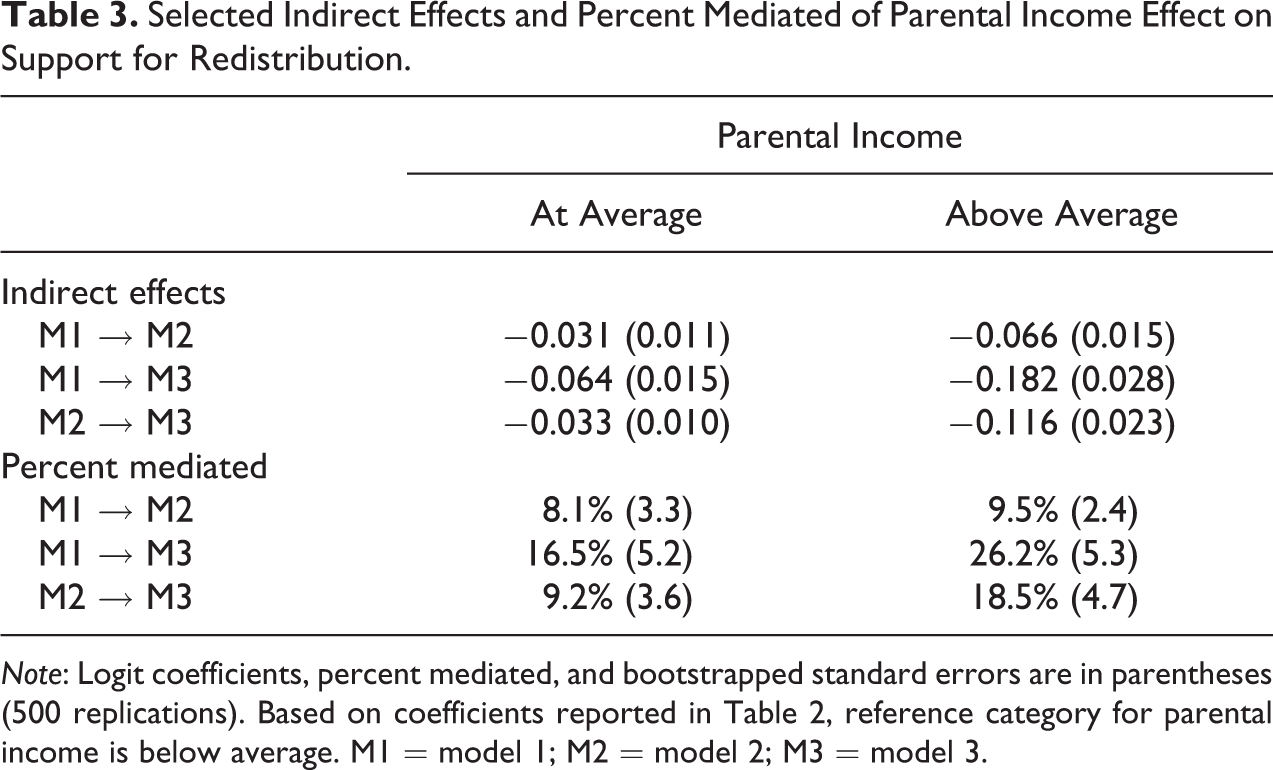
Note: Logit coefficients, percent mediated, and bootstrapped standard errors are in parentheses (500 replications). Based on coefficients reported in Table 2, reference category for parental income is below average. M1 = model 1; M2 = model 2; M3 = model 3.

Conclusion

The KHB method has rapidly become popular. In this note, we have provided, and illustrated, a reformulation of the method, which, we believe, is simpler to implement than that used in the original paper and implemented in the Stata program, khb,⁴ Kohler, Karlson, and Holm (2011). It has particular advantages when we want to consider how the association between a categorical or ordered outcome and a predictor variable of interest changes when we add several mediators or confounders sequentially

Supplemental Material

Online_Appendix - A Note on a Reformulation of the KHB Method

Online_Appendix for A Note on a Reformulation of the KHB Method by Richard Breen, Kristian Bernt Karlson and Anders Holm in Sociological Methods & Research

Footnotes

Declaration of Conflicting Interests

The author(s) declared no potential conflicts of interest with respect to the research, authorship, and/or publication of this article.

Funding

The author(s) received no financial support for the research, authorship, and/or publication of this article.

Supplemental Material

Supplemental material for this article is available online.

Notes

References

Breen

Richard

Karlson

Kristian Bernt

Holm

Anders

. 2013. “Total, Direct, and Indirect Effects in Logit and Probit Models.” Sociological Methods and Research 42:164–91.

Breen

Richard

Karlson

Kristian Bernt

Holm

Anders

. 2018. “Interpreting and Understanding Logits, Probits, and Other Non-Linear Probability Models.” Annual Review of Sociology 44:39–54.

Karlson

Kristian Bernt

Holm

Anders

Breen

Richard

. 2012. “Comparing Regression Coefficients between Same-sample Nested Models Using Logit and Probit: A New Method.” Sociological Methodology 42:274–301.

Kohler

Ulrich

Karlson

Kristian Bernt

Holm

Anders

. 2011. “Comparing Coefficients of Nested Nonlinear Probability Models.” The Stata Journal 11:420–38.

Supplementary Material

Please find the following supplemental material available below.

For Open Access articles published under a Creative Commons License, all supplemental material carries the same license as the article it is associated with.

For non-Open Access articles published, all supplemental material carries a non-exclusive license, and permission requests for re-use of supplemental material or any part of supplemental material shall be sent directly to the copyright owner as specified in the copyright notice associated with the article.

0.00 MB

0.18 MB