
Abstract
Nonlinear mixed-effects models are models in which one or more coefficients of the growth model enter in a nonlinear manner, such as appearing in the exponent of the growth function. In their applications, the within-individual residuals are often assumed to be independent with constant variance across time, an assumption that implies that the assumed growth function fully accounts for the dependencies and patterns of variation in the data. Studies have shown that a poorly specified within-individual residual covariance structure of a linear mixed-effects model can impact the estimated covariance matrix of the random effects at the second-level, model fit and statistical inference. The consequences for nonlinear mixed-effects models are not, however, clearly understood. This is due in part to the differences in the estimation needs of the two types of models. Using empirical data examples, this work illustrates the impact of fitting alternative residual covariance structures in nonlinear mixed-effects models that do not entirely parallel the results from studies of strictly linear mixed-effects models and call for the need of researchers to consider alternative structures when fitting nonlinear mixed-effects models.
Keywords
Accounting for dependencies and heterogeneity of variance in longitudinal data is central to fitting mixed-effects models. Although a particular growth model may account for much of the within-individual variation and covariation in a longitudinal response, some dependencies may remain or the assumption of homogeneity of variance may not be met. Not accounting for dependencies in the residuals at the first level of a mixed-effects model that is strictly linear in its parameters has been shown to result in poorer model fit and biased parameter estimates (Chi and Reinsel 1989; Ferron, Daily, and Yi 2002; Kwok, West, and Green 2007; Sivo, Fan, and Witta 2005). The impact of not accounting for heterogeneity of variance in the residuals may have similar implications. With the consequences of a poorly specified residual covariance structure well understood for linear mixed-effects models, steps to assess the adequacy of the structure are commonly outlined in articles and books describing the general methodology (Muthén 1997; Raudenbush and Bryk 2002; Singer and Willett 2003) and applied in practice (Roberts and Adams 2018; Wickrama, Lorenz, and Conger 1997).
Nonlinear mixed-effects models, in which one or more of the growth coefficients enters the function in a nonlinear, or nonadditive, way, are inherently more complex than those within the family of linear mixed-effects models (Davidian and Giltinan 1995, 2003). Nonlinear mixed-effects models differ from the linear version in several important ways. Perhaps one of the most important differences is that the former provides a highly flexible means of modeling longitudinal data. That is, longitudinal data that follow complex forms of change, such as data that tend toward an asymptote or that follow multiple phases of change, require a nonlinear modeling framework that allows for any specified form of growth. Although linear mixed-effects models can be used to model some complex forms of change, such as by applying a quadratic or cubic growth function to capture nonlinear change, linear mixed-effects models are limited to polynomial functions that may not provide an intuitive understanding of a longitudinal process. Conversely, nonlinear mixed-effects allow for a longitudinal process to be modeled by any kind of function. This can be ideal for directly relating aspects of growth or change to hypotheses about a longitudinal process (Cudeck 1996; Fitzmaurice, Laird, and Ware 2004).
Given the complexity of some longitudinal data, it can be challenging to define a growth model that adequately captures a longitudinal process. Although a quadratic growth model may approximate some forms of nonlinear change, it may not do well in characterizing a process that tends to level off with time. Alternatively, an exponential growth function may improve upon the characterization of such a process. More complex models can be anticipated for responses expected to follow multiple phases of change over time, such as the bereavement response to the loss of a spouse (Infurna et al. 2017), and so a model that allows for transitions between different response functions over the course of time may be necessary. In any case, there is likely to be some degree of misfit between the observed longitudinal response and the hypothesized form of change, especially given that a hypothesized model serves at best to approximate a behavior. Although this issue is a problem common to both linear and nonlinear models, the problem may be greater when fitting nonlinear models because their applications naturally involve more complex forms of change (e.g., Lee and Rojewski 2009; Zhao et al. 2016). Thus, concerns about dependencies in the residuals, as well as heterogeneity of variance, at the first level of a nonlinear mixed-effects model may play a greater role when considering these models simply given their greater complexity.
Adding to the complexity in fitting nonlinear mixed-effects models are cases where longitudinal data are incomplete and the source of the missing data is not ignorable (Xu and Blozis 2011). Although mixed-effects models allow for missing response data in longitudinal studies, if the source of the missing data is not ignorable, more complex modeling procedures are needed (Molenberghs and Kenward 2007). Nonignorable sources of missing data can compromise statistical inference from a model, and consequently, erroneous conclusions about the data may be drawn. One of the problems with nonignorable missingness is that it can be an additional source of dependency in the data or heterogeneity of variance, that if not addressed, can mean that an assumption of independent residuals or homogeneity of variance will not be met. In some cases, a covariate that is related to the missingness can be included in the model, and the missingness is then ignorable. If, however, such covariates are either not available or do not adequately address the source, then a model that accommodates greater flexibility in the residual covariance structure can be an important aspect of fitting a model to ensure valid statistical inference.
Unlike a nonlinear mixed-effects model, it is actually possible to generate an analytic solution to possible consequences of a misspecified within-individual residual structure under a linear mixed-effects model. For both linear and nonlinear mixed-effects models, the marginal distribution of the response is a multidimensional intergral of the joint distribution of the response and the random effects (Davidian and Giltinan 2003). For a linear mixed-effects model, integration of the integral can be handled algebraically, and the result is a closed-form solution for the marginal distribution of the response. Given this, it is possible to provide an analytic solution to possible consequences of a misspecified within-individual residual structure in which parameters that characterize the random effects covariance structure are impacted (see Online Appendix A). The same, however, is not true for a nonlinear mixed-effects model that includes a nonlinear random effect because the integration of the integral cannot generally be done algebraically, making it not possible to carry out a solution like can be done for the linear model. With this, it is not possible to use this strategy to understand the potential consequences of a misspecified residual covariance structure. Thus, although the issues that arise when fitting linear mixed-effects models may be thought to arise as well when fitting nonlinear mixed-effects models, it is not possible to derive an analytic solution to understand the potential problems, particularly with regard to the random effects. Further, given the great complexity of formulating and estimating nonlinear mixed-effects models, it is not clear whether the consequences that have been documented for linear mixed-effects models parallel those for nonlinear mixed-effects models.
In practice, choosing among alternative residual covariance structures for a linear mixed-effects model is straightforward using commercial software programs, such as SAS PROC MIXED, that include several options. Using the TYPE option in the REPEATED statement of PROC MIXED, for instance, users can specify one of the many available covariance structures, such as a first-order autoregressive structure or heterogeneity of variance. Conversely, programs for fitting nonlinear mixed-effects models, such as SAS PROC NLMIXED, do not readily offer such options. Harring and Blozis (2014) showed how PROC NLMIXED could be used to fit a nonlinear mixed-effects model for which the within-individual residual covariance structure allows for correlations between residuals or for heterogeneity of variance. This is accomplished by relying on the GENERAL loglikelihood option in the MODEL statement. With this, researchers may more readily consider how alternative residual structures can impact model fit and the parameter estimates of the model. Nonlinear mixed-effects models provide for a greater range of functional forms for longitudinal data relative to linear mixed-effects model, and so understanding the impact of fitting alternative residual structures is important, as nonlinear mixed-effects model increase in popularity across many domains of study in the social and behavioral sciences, especially in light of recent applications of nonlinear mixed-effects models that do not consider alternatives to the standard assumption of independence of the within-individual residuals with constant variance (Marceau, Abar, and Jackson 2015; Zhao et al. 2016).
This article evaluates the use of alternative covariance structures for longitudinal data fit by a nonlinear mixed-effects model with a focus on model selection, model fit, and sensitivity of parameter estimates under different assumptions about the within-individual residual covariance structure. This article extends earlier work in a number of ways. First, we consider data from a learning study presented in Harring and Blozis (2014). In Harring and Blozis, many different functions were applied to the learning data, and model fit comparisons were done for models that all assumed the level 1 residuals were independent with constant variance. Here, we consider these data to see whether different residual covariance structures should also be consider during the process of selecting a growth function to describe the data. A central assumption about a mixed-effects model is that the chosen function, such as a logistic versus an exponential growth function, represents the general form of change for all individuals in a population with subject-specific coefficients that allow for individual differences in specific aspects that characterize change. The residuals at the first level of the model represent the discrepancies between the fitted model and the data. One question is whether alternative residual covariance structures should be consider during the process of selecting a growth function to provide insight into the process of providing a suitable representation of the data. Also in Harring and Blozis’s work, a first-order autoregressive residual structure was shown to provide a superior fit to the learning data relative to the fit of a model that assumed independent residuals with constant variance and other residual structures, but it was not shown how this preferred residual structure impacted parameter estimates and statistical inference. We, therefore, aim to also study the impact of these assumptions on model inference.
We also extend earlier work by considering problems of incomplete longitudinal data and for which the missingness (i.e., whether data are missing or not) may not be ignorable. Parameter estimates from a mixed-effects model are unbiased if the source of the missing data is ignorable, such that the missingness is independent of the missing values (Laird 1988). One approach to addressing nonignorable missingness in a mixed-effects model is to incorporate indicator variables that represent patterns of missing data. In a random-effects pattern-mixture model, indicator variables are included in the model to account for between-subject variation in the random effects, which is attributable to patterns of missing data. Conditional on these patterns, the missingness is assumed to be ignorable (Little 1995). Based on prior work on linear mixed-effects models in which the use of alternative residual covariance structures was studied, it is understood that changes in the assumptions about the residual covariance structure at the first level of the model can lead to changes in the covariance structure of the random effects at the second level (Chi and Reinsel 1989). Thus, this article explores the impact of fitting alternative residual covariance structures in the context of fitting a nonlinear random-effects pattern-mixture model. If, for instance, data are best fit with a model that uses an alternative residual covariance structure and this results in a change in the covariance structure of the random effects at the second level of the model, then this could possibly lead to changes in the pattern-mixture model component that serves to address nonignorable missingness.
In fitting models to the different data sets, we provide maximum likelihood (ML) estimates (see Harring and Blozis 2014) and Bayesian estimates. Bayesian estimation vis-à-vis Markov chain Monte Carlo (MCMC) methods (Gelfand and Smith 1990; Wakefield 1996) of hierarchical models such as the nonlinear mixed-effects models provides an alternative scheme to ML (Davidian and Giltinan 1995) that, in contrast, relies on large-sample asymptotic results based on normal theory for valid statistical inference. For data sets using small samples, it is often difficult to ensure such approximations of the sampling distributions of parameter estimates are valid (De la Cruz-Mesia and Marshall 2006). In addition, the uncertainty of parameter estimates and future predictions are relatively difficult to evaluate under ML, especially in cases for which general model assumptions such as independent residuals and normality are relaxed (Li, Stewart, and Weiskittel 2012). Thus, the primary benefits of using a Bayesian approach include its ability to generate the full posterior distribution of estimated parameters through samples generated by simulation algorithms during model fitting from which various statistics (mean, mode, median, SD, etc.) can be easily calculated (Levy and Mislevy 2016). As we provide results using both methods of estimation, this allows for comparisons between sets of results to study the sensitivity of estimates to the different approaches to estimation. We note as well that many applications of nonlinear mixed-effects models using Bayesian estimation take the approach of a simple specification of the residual covariance structure like a conditionally independent structure with constant variance, and so structures that allow for serial correlation within a Bayesian framework are rare (Broemeling 2016).
The remainder of this article is as follows: For background, mixed-effects models are reviewed first. A set of residual covariance structures is then described that allow for correlations between residuals and heterogeneity of variance. Similar to Harring and Blozis (2014), among others who have studied this problem for linear mixed-effects model (e.g., Kwok et al. 2007), longitudinal measures are assumed to be assessed at discrete points in time. Two empirical data sets are then described and analyzed to study the impact of different residual structures. In each example, a set of nonlinear mixed-effects models that are judged as suitable contenders in describing the longitudinal data is applied along with different residual structures to address possible dependencies and heterogeneity of variance in the data conditional on the assumed individual-specific growth function. Fitting the alternative residual structures provides a means of evaluating the standard assumption that the residuals are independent with constant variance, as well as understanding the impact of this assumption on model fit and the estimated parameters.
Mixed-effects Models
Mixed-effects models are a major tool for the analysis of longitudinal data due to their emphasis on the individual, as well as the flexibility in how the models may be specified. A common function is selected to describe the responses of individuals in a population, but the particular coefficients of the function, such as the rate of change, may be unique to the individual. That is, all individuals in a population are assumed to follow the same functional form, but the parameters of the growth function can vary between individuals. The fact that the model can be formulated to highlight individual differences in the characteristics that describe change has made these models widely popular in many disciplines of study. Although applications of linear mixed-effects model that are based on polynomial functions (Raudenbush and Bryk 2002) are clearly predominant in the behavioral sciences, the need for nonlinear mixed-effects model to characterize measures that change at nonconstant rates is obvious in several areas of study such as learning, development, and personality. For example, longitudinal responses from these types of studies can follow forms of change that are best described by a growth function that includes an asymptote (Choi, Harring, and Hancock 2009) or possibly by two or more growth functions that are linked together to allow for distinct phases in change (Cudeck and Klebe 2002; Kohli and Harring 2013; Zhao et al. 2016).
For instance, common to learning data are responses that tend toward an upper or lower asymptote (e.g., Susman et al. 1998). In developmental studies that are carried out over extended periods of time, a response can tend to follow one course (e.g., increasing linear growth) and then shift to a different course (e.g., decreasing linear growth) (Schlotz et al. 2011). Problems such as these often require a nonlinear growth model to account for complex patterns in the data. Also of value, nonlinear models can be specified to yield a parsimonious model based on highly interpretable parameters (Cudeck 1996). Indeed, the need for nonlinear growth models is apparent in majors areas of behavioral study including development (Burke, Shrout, and Bolger 2007; Grimm, Ram, and Hamagami 2011; Laursen, Little, and Card 2013; Roberts 1986) and personality (West et al. 2011). Choi et al. (2009), for example, describe the utility of a logistic function to understand longitudinal data that follow an S-shaped form of change. They emphasize the appealing aspects of using a nonlinear function to capture meaningful features of a measured response such as an asymptote to represent the long-run tendency of a response.
We first review a mixed-effects model for a normal variable in which the growth function can be nonlinear, or nonadditive, in its parameters. Let

where
At the first level of the model, the residual
where
Accounting for Within-individual Dependencies
An essential part of formulating a longitudinal model is accounting for the within-individual dependencies in the data, given that longitudinal data are typically autocorrelated within person. A mixed-effects model addresses these dependencies by assuming that at least part of the dependencies is due to person-specific function parameters. As an example, the responses of individuals from a population may all tend to follow the same nonlinear form of growth such as a logistic curve (Choi et al. 2009), but growth at the individual level may vary, with individuals having unique response levels and unique rates of change. A mixed-effects model includes subject-specific coefficients that allow the fitted growth curves to better align with an individual’s response. Given a suitable growth model, variation in the responses may be well accounted for by the growth function that includes the subject-specific coefficients, and as a result, the residuals conditional on the subject-specific growth model are independent. In such cases, it would then be appropriate to interpret a model that assumes that the residuals are independent between measurement occasions and possibly that the variances of the residuals are constant over time. If, however, some correlations in the residuals remain, this may be an indication that the chosen function is not adequate in summarizing the responses or that additional covariates may be needed to address the dependencies. In either case, inference from a model that assumes that the within-individual residuals are independent may be problematic. Thus, the ability to model dependencies in data not fully captured by an assumed growth function may be important, particularly for situations in which the source of the dependencies is not well understood, such as when additional covariates are not available to address the dependencies. In these latter cases, the only recourse may be to specify a covariance structure that simply allows for correlations between the residuals at different occasions. In other kinds of problems, it may be that the assumption of homogeneity of variance is not tenable, and for these cases, it might be appropriate to allow for heterogeneity in the variances of the residuals. Although either of these situations is more commonly considered for applications of linear mixed-effects model, the same is not true for nonlinear mixed-effects models (Harring and Blozis 2014).
Related to the need for alternative residual covariance structures in fitting nonlinear mixed-effects model are the analytic methods that are required for estimation of these models. That is, there can be practical challenges in the estimation of nonlinear mixed-effects model in general, a problem that quite often is due to a nonlinear random coefficient. Estimation of a nonlinear mixed-effects model that includes a nonlinear random coefficient can present a challenge because the likelihood function for a given model may not be tractable, meaning that it is not possible to express the likelihood function in such a way as to directly solve for the parameters. For a linear mixed-effects model, for instance, a likelihood function may be reexpressed as a log of the likelihood function, and differential calculus applied to obtain an analytic solution. Commonly applied algorithms, such as Newton-Raphson, may then be implemented in a straightforward manner to obtain parameter estimates. For a nonlinear mixed-effects model, much effort has been made to develop methods to solve this often complex estimation problem. Solutions include methods that rely on linear approximations to a nonlinear function, such as a first-order Taylor series approximation (Beal and Sheiner 1982; Pinheiro and Bates 1995). Alternatively, if the nonlinear coefficients are fixed across individuals and only coefficients that enter the function in a linear way are random, then estimation may be carried out using methods commonly used for estimation of linear models (Blozis 2007; Blozis and Cudeck 1999). Thus, a central issue seems to concern problems for models that include nonlinear random effects.
PROC NLMIXED is employed for the estimation of nonlinear mixed-effects models with the assumption for normally distributed data that the residuals are independent with constant variance. As described, estimation of a nonlinear mixed-effects model is rather complicated, and much of the literature has focused on available approaches and consequences to their choices (e.g., Harring and Blozis 2016). To date, the program does not include options for the within-individual residual structure. So, unlike PROC MIXED that provides for many options for the residual covariance structure, the same is not true of PROC NLMIXED. Due to Harring and Blozis (2014), it is possible to use SAS PROC NLMIXED to fit several alternative within-individual covariance structures of a nonlinear mixed-effects model that includes nonlinear random effects. This can be done by implementing the MODEL statement with the GENERAL option in which users provide a loglikelihood function with direct specification of both the mean function and the covariance structure of a given model. As detailed in Harring and Blozis (2014), a multivariate normal density function requires both the inverse and the determinant of the within-individual covariance structure. To allow for serial correlation, for instance, the variance matrix of the level 1 residuals is separated from a matrix that represents the serial correlations among the residuals (see Davidian and Giltinan 2003). In the expression of the density function, the within-individual covariance matrix is constructed by combining the inverse and determinant of the variance matrix and correlation matrix. With this general strategy, it is possible to fit patterned matrices that include a first-order autoregressive structure, a symmetric banded-1 Toeplitz structure, compound symmetry, and an independent structure with nonconstant variance.
Alternative Residual Covariance Structures
In fitting a growth model to data for which the rate of change in the response is not constant over time, there may be several functions considered to be suitable for describing the data. Learning and developmental processes, for instance, may be well summarized by a function that allows for the responses to tend toward an asymptote. Functions of this kind may include any member of the Richards (1959) family of functions such as a logistic, exponential, or Gompertz function. A response may be assumed to follow a function that relies only on time, or the function may additionally include covariates such as time-varying covariates in which a response is assumed to be due to time along with variables that also change with time. Naturally, moderators (i.e., predictors) of the coefficients of a given function may be incorporated into the model, such as allowing person-level attributes to moderate the change rate or response level. In practice, one may fit several suitable functions both with and without covariates and evaluate model fit between them.
A measure of how well a model accounts for the responses is the within-individual residuals, that is, the discrepancies between an individual’s observed scores and those predicted by a model. Relatively large residuals can suggest a poor fitting model to a competing model. Among a set of fitted models, the one that yields the smallest average residual may be judged as best. Even with the best fitting of a given selection of models, it may be that some degree of correlation between the residuals remains, a result that would suggest that the chosen function did not fully account for the within-individual dependencies in the data. The source of the correlation may be known, in which case covariates may be added to the model to help address the dependencies, or the source may be unknown, in which case one may only be able to allow for correlations between the residuals. In a different situation, it may be that the variances of the residuals are not equal across the different time points. Similar to addressing correlations between residuals, addressing differences in the residual variances may be done by introducing covariates into a model or by specifying a model that allows the variances to differ.
Simulation studies have investigated the impact of ignoring correlated residuals in linear growth models (Ferron et al. 2002; Kwok et al. 2007; Sivo et al. 2005) and have shown poorer model fit and biased estimates of the variances and covariances of the random effects for conditions under which the level 1 residuals were assumed to be independent with constant variance. Depending on the particular software that is used to fit a linear model with random effects, there may be several different options available for the residual structure. SAS PROC MIXED, as noted earlier, offers many options for covariance structures. Latent growth models fitted within a structural equation model framework can also handle heterogeneity of variance as well as covariances between residuals (e.g., Willett and Sayer 1994). Thus, not only does the option of fitting alternative residual structures allow for possible improvement in model fit and parameter estimates, it allows for assessments of the tenability of the commonly assumed structure of conditional independence and homogeneity of variance.
For nonlinear mixed-effects model, Harring and Blozis (2014) develop syntax for PROC NLMIXED to fit several alternative residual structures that are more typically used in fitting linear mixed-effects model. These structures include one that allows heterogeneity in the residual variances over time, assuming that the residuals are independent between occasions. Other structures allow for correlations between the residuals and include a first-order autoregressive structure, compound symmetry, and a symmetric banded-1 Toeplitz structure. These residual structures are briefly reviewed here. As in many applications of linear mixed-effects model, these particular residuals structures are applied to discrete measures of time such that there is a common set of measurement occasions across individuals, although some individuals may not have complete data for all occasions. The residual covariance structures presented in Harring and Blozis’s work are shown here assuming four measurement occasions. Naturally, these structures can be generalized to handle a different number of measurement occasions.
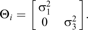
Heterogeneity of Variance
A residual covariance structure
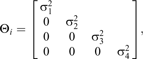
where the subscript on the variances denotes the four distinct variances at each occasion. Additionally, the subscript
Autoregressive Residual Structure
A first-order autoregressive residual structure allows for the residuals between adjacent time points to covary and assumes that the magnitude of the correlation lessens as scores move further apart in time:

where
Compound Symmetry
Compound symmetry assumes that the residuals have constant variance across time, and the covariances between the residuals maintain a constant magnitude no matter how far apart the measures lie with regard to the measurement occasions:

where
Symmetric Banded-1 Toeplitz Structure
A version of a banded-1 Toeplitz structure is one in which the variances are constant and the covariances between residuals separated by one time lag are equal, and all other covariances are set equal to 0:
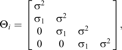
where
Examples
The first example comes from a learning study in which performance measures were obtained over a series of consecutive trials within a single study session. Models for learning data may benefit from consideration of alternative residual covariance structures to adequately capture patterns in the data. That is, although a nonlinear mixed-effects model, such as one based on an exponential growth function that includes an asymptote, may do well in accounting for individual differences in the responses across trials by including subject-specific growth coefficients, it is possible that after fitting the model that the trial-specific residuals may be correlated within person. This can result if an individual’s responses do not change entirely according to the specified growth function and perhaps a different function is warranted. Thus, finding that some correlation between the residuals remains after fitting a model may suggest the need for an alternative growth model, such as one that uses a different function or one that includes time-varying covariates. It may also be that the residual variances are not equal across trials. Differences in residual variances across trials could reflect a number of possible sources. For example, the within-individual variation toward the end of the study trials could increase due to participant fatigue for some participants and not for others. Alternatively, some participants may show greater stability in performance toward the end of the learning trials that would be reflected as a decrease in variation for them but not for others. We explore such possibilities for the learning data. The second example is from a study of clinical status for a sample of individuals diagnosed with schizophrenia. For these data, responses were recorded weekly although some data are missing. Valid inference from a mixed-effects model requires that the source of the missing data is ignorable. Previous analyses of these data using linear mixed-effects models suggest that the source of the missing data may not be ignorable (Hedeker and Gibbons 1997). Here, a nonlinear random-effects pattern-mixture model is applied to account for nonignorable missingness and is further evaluated under alternative assumptions about the residual covariance structure. Of particular interest for these data is whether the assumptions made about the residual covariance structure have any impact on the conclusions drawn about the missing data.
In considering alternative residual covariance structures, a sensitivity analysis is performed in each of the examples to evaluate the parameter estimates of the growth models under different assumptions about the residual structure. The purpose of doing such an investigation follows from work on linear mixed-effects models. For instance, Chi and Reinsel (1989) describe how changes in the assumptions about the residual covariance structure at the first level of a linear mixed-effects model can lead to changes in the estimated covariance structure of the random effects at the second level of the model. Specifically, they discuss that in a linear mixed-effects model, the random effects may represent serial correlation between measures within person and that a first-order autoregressive structure combined with random-effects may be more appropriate in such cases. Here, we study the impact of applying these alternative residual covariance structures on model specification and statistical inference of nonlinear mixed-effects models.
In addition to studying the sensitivity of parameter estimates under different assumptions about the residual covariance structure, comparisons are made with regard to the estimation method. As discussed previously, estimation via ML relies on large-sample asymptotic results based on normal theory for valid statistical inference, making it difficult to ensure valid approximations of the sampling distributions of parameter estimates when sample sizes are not large (De la Cruz-Mesia and Marshall 2006). The benefits of using a Bayesian approach include the ability to generate the full posterior distribution of estimated parameters through samples generated by simulation algorithms during model fitting. Comparing results obtained via ML and Bayesian thus allows for evaluation of the sensitivity of results to the chosen estimation methods. Here, ML estimation was carried out using PROC NLMIXED with SAS version 9.4. The Bayesian analyses were executed using WinBUGS software version 1.4.3. (Spiegelhalter et al. 2002), a widely adopted program for Bayesian analysis in which estimated parameters may be obtained from their posterior distributions using MCMC algorithms. We used the R packages BRugs (Thomas 2004) and R2WinBUGS (Sturtz, Ligges, and Gelman 2005) to link R and WinBUGS for data input and output and graph generation for convergence diagnostics. Syntax for fitting models to the learning data in provided in the Online Appendix B.
Performance on a Flight Simulation Task
Data from a computerized skill acquisition task that was presented in Kanfer and Ackerman (1989; also see Harring and Blozis 2014) are studied here. The data represent the number of planes brought in safely for a series of ten 10-minute intervals, a task designed to simulate the role of an air traffic controller. Participants were allowed ten-minute breaks immediately following the fourth and seventh trials. The data are the performance measures for 140 participants. Data from the first interval were excluded from analysis assuming that the measures could reflect the participants’ adjustments to the task. Sample means and the covariance matrix of performance scores for the nine intervals (
Similar to Harring and Blozis (2014), we considered functions that allow for an upper asymptote. Specifically, we fit models using an exponential and a logistic function (cf. Browne 1993):


The function coefficients include random effects so that the functions are specific to each participant (with the random effects assumed to covary with each other). As described in Browne (1993), these particular forms of an exponential and logistic function have parameters that have essentially the same interpretation. Thus, for both functions,
For a set of models that assume the same growth function (i.e., either logistic growth or exponential growth), the different residual structures reviewed earlier were applied to understand whether assumptions made about the residuals play a role in the selection of a growth model for these data. As a set, the alternative residual structures provide a means of assessing the assumptions that the residuals are independent and that their variances are constant across trials. The models were estimated using the default method for PROC NLMIXED, Gauss–Hermite quadrature, that is implemented by using the GENERAL loglikelihood option in the MODEL statement. Syntax for fitting a nonlinear mixed-effects model with these alternative residual structures is provided by Harring and Blozis (2014). Additionally, the noad (for nonadaptive Gaussian quadrature) option was selected. Estimates were based on 30 quadrature points. Lesaffre and Spiessens (2001) and Pinheiro and Bates (1995) discuss the role of specifying the number of quadrature points when applying adaptive and nonadaptive Gaussian quadrature. Starting values were generated by first fitting a completely fixed-effects model to obtain fixed-effects estimates and a constant residual variance at level 1. Using those results as an updated set of starting values, we added in a stepwise fashion random effects to the second level of the model, beginning with a random intercept, then a random asymptote, and finally a random rate parameter. Starting values were updated with each step. In a final step, the final model that was deemed to provide the best fit to the data was fit again using Bayesian estimation methods. Bayesian estimates for the best fitting growth model, as well as a model that assumed that the residuals were conditionally independent with constant variance, are provided. Details regarding specific assumptions made for the Bayesian estimation are provided in Online Appendix C.
Results
Indices of model fit based on ML estimation are in Table 1. In addition to −2 times the loglikelihood, we report the Akaike information criterion (AIC; Akaike 1974) and the Bayesian information criterion (BIC; Schwarz 1978). Smaller values of the AIC and BIC indicate preferred models in terms of relative model fit. Across models, the logistic function was preferred over the exponential function regardless of the assumptions made about the residual structure. This suggests that for these data, the choice of a growth function was not sensitive to changes in the assumptions about the within-individual residuals. Thus, the pursuit of selecting a suitable nonlinear growth function for these data does not seem to require that different residual covariance structures be considered throughout the process.
Indices of Model Fit for Performance Scores on a Flight Simulation Task using ML Estimation.

Note: n = 140. Models were fit using ML via nonadaptive Gaussian quadrature and 30 quadrature points. ML = maximum likelihood.
For either growth function, model fit was most improved if a first-order autoregressive residual structure was assumed, suggesting that dependencies in the data remain after fitting the growth function. The fact that the other residual structures did not improve model fit to the same extent or greater sheds light on the learning response and is worth exploring. Specifically, using the AIC value to evaluate the relative fit of compound symmetry to the independent structure, there was a slight improvement in model fit, whereas the BIC suggests that the added complexity of compound symmetry provided no improvement. Although compound symmetry allows for scores to covary over time, the added restriction that the dependencies are constant across all covariances, regardless of the distance between trials, is not consistent with the data. The symmetric banded-1 Toeplitz model improved model fit, but comparisons of model fit suggest that the assumption that scores two or more trials apart are independent is not consistent with the data. The structure that assumes independence between residuals and different residual variances across trials improved model fit as well but not to the same extent as the first-order autoregressive structure. The fact that the first-order autoregressive structure provided relatively the best overall fit suggests that the need to address decreasing dependencies in the residuals across trials was most important and addressing possible differences in the residual variances was not. Consistent with studies involving linear mixed-effects model, model fit for nonlinear mixed-effects models may be improved by relaxing the usual assumption that the residuals are independent with constant variance (Chi and Reinsel 1989).
Table 2 reports the estimated fixed effects and variances and covariances of the random coefficients based on the logistic growth model assuming that the residuals are independent with constant variance and then assuming a first-order autoregressive (AR[1]) structure. Sensitivity of estimates to assumptions about the within-individual errors is studied by making comparisons between the estimates, giving light to the impact that this alternative structure has on model inference. Bayesian estimates for these two models are provided as well. As shown in Table 2, there are slight differences in the estimated fixed effects between models and estimation methods, so conclusions regarding the typical performance trajectory are fairly consistent across models and estimation methods. Thus, the assumptions about the residual covariance structure seem to have little impact on the report of the typical performance trajectory.
ML and Bayesian Estimates of a Logistic Growth Function Under Independence Versus First-order Autoregressive (AR(1)) for Performance Scores on a Flight Simulation Task.
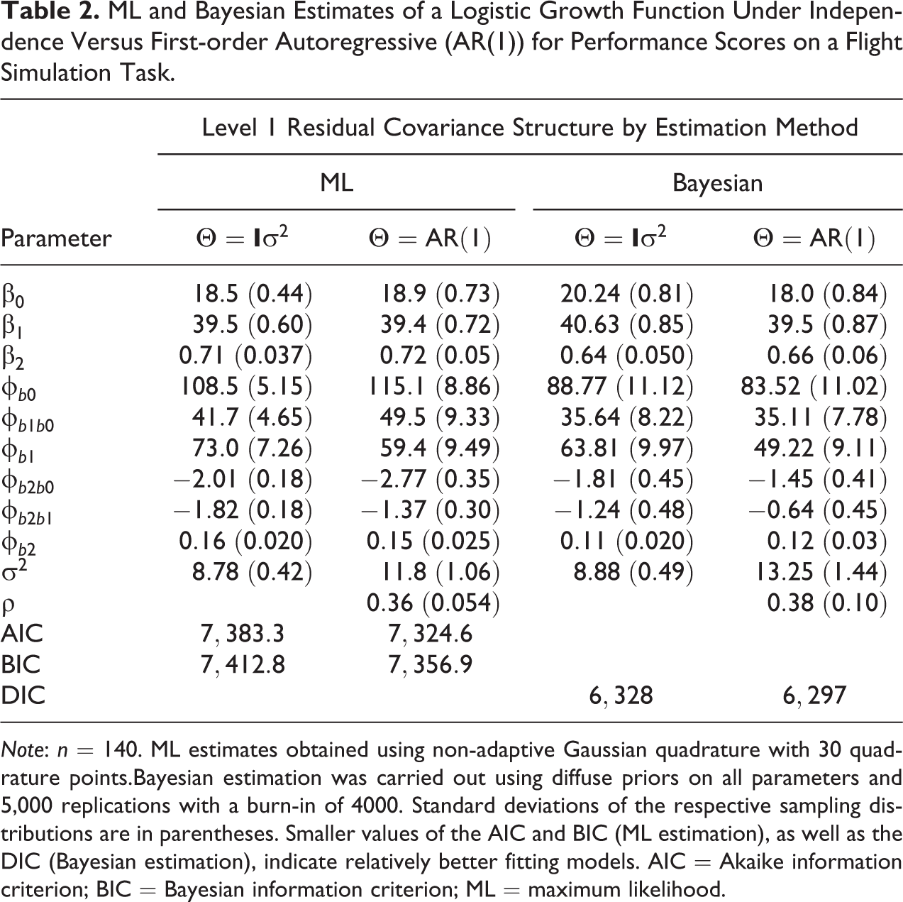
Note: n = 140. ML estimates obtained using non-adaptive Gaussian quadrature with 30 quadrature points.Bayesian estimation was carried out using diffuse priors on all parameters and 5,000 replications with a burn-in of 4000. Standard deviations of the respective sampling distributions are in parentheses. Smaller values of the AIC and BIC (ML estimation), as well as the DIC (Bayesian estimation), indicate relatively better fitting models. AIC = Akaike information criterion; BIC = Bayesian information criterion; ML = maximum likelihood.
Perhaps the more important differences between models are in the estimated variances of the random effects. Using ML, the estimated variance of the random intercept
Severity of Illness Ratings
Data from the National Institute of Mental Health Schizophrenia Collaborative Study are studied in an application of a nonlinear mixed-effects model for which different mean and covariance structures are considered. The data are based on Item 79 of the Inpatient Multidimensional Psychiatric Scale (Lorr and Klatt 1966), a seven-point ordinal scale measuring severity of illness: 1 = normal, not at all ill; 2 = borderline mentally ill; 3 = mildly ill; 4 = moderately ill; 5 = markedly ill; 6 = severely ill; and 7 = among the most extremely ill. Data are available for 437 patients for whom weekly severity ratings were planned for up to six weeks in addition to a baseline measure, with all patients having some missing data. Table 3 displays the sample descriptives of the severity ratings for week
Summary Statistics of Weekly Severity of Illness Ratings by Placebo Versus Drug.

Note: N = 437.

A plot of severity of illness ratings for a subsample of 20 individuals (drug group upper plot; placebo group lower plot).
In a longitudinal study, whether data are missing or not may be related to the missing data. In such cases, the missingness is said to be nonignorable. Consequently, inference from a longitudinal model without accounting for the missingness may be misleading (Molenberghs and Kenward 2007). Thus, an important goal for the data analysis here was to address a potential source of nonignorable missingness due to attrition, as has been considered for these data in previous studies that relied on linear mixed-effects models that assumed independence and constant variance for the residuals (Hedeker and Gibbons 1997). This is done here in the context of fitting a nonlinear mixed-effects model, in addition to fitting different residual covariance structures. Following Hedeker and Gibbons (1997), the measures are first studied as a function of time, measured in weeks, in addition to a treatment indicator variable that denoted whether a patient received one of four psychiatric medications (drug
As a first step in the analysis, different growth functions that included drug
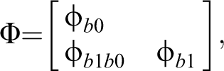
Using the logistic growth model to describe illness ratings, dropout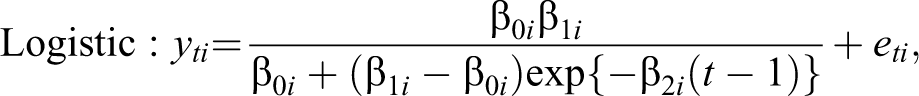
where


and with
Next, models assuming ignorable missingness conditional on
It is important to note that it is not possible to confirm with absolute certainty the role that missingness plays in statistical inference (Molenberghs and Kenward 2007). This is due to the fact that analyses are conducted using only observed data. The missing data are not available to conduct any test concerning a relationship between the missing data and the missingness, and the missingness itself may not be fully understood simply by examination of the observed data. Thus, a common goal for an analysis that includes some information about the missing data process is to evaluate the conclusions drawn from an analysis that is based on assumptions that are made about the missing data. Generally, it may be best practice to consider multiple mechanisms that may explain the missing data, keeping in mind that the actual missing data process may not be correctly specified (simply because it is not likely to be known). Thus, although we provide values of the AIC and BIC for the different models fitted using ML, one must be cautious in drawing conclusions about the missing data mechanism. As an added note, the BIC, unlike the AIC, uses sample size in its calculation. SAS PROC NLMIXED calculates the BIC as: BIC =
Results
For each model that differed according to the residual covariance structure, the three coefficients of the logistic function that included
Model Fit for a Logistic Growth Function Applied to Psychiatric Illness Severity Ratings Under Different Missing Data Assumptions Using ML Estimation.

Notes: n = 437. q is the number of model parameters. Models were fit using ML via nonadaptive Gaussian quadrature and 30 quadrature points. Smaller values of the AIC and BIC indicate relatively better model fit.
Table 5 provides ML estimates of the logistic growth models under ignorable and nonignorable missingness, as well as assuming that the residuals were independent with constant variance and independent with nonconstant variance.1 The fixed effects estimates that relate to the initial response and the rate parameter are fairly comparable between models that make the same assumption about the missingness, suggesting no appreciable impact of this assumption on the initial response and rate of change for the typical individual under each assumption about missingness. Depending on whether the residuals were assumed to be independent with constant variance or with nonconstant variance, we note differences in the estimates relating to the effects of covariates on the asymptote under the assumption of nonignorable missingness but not ignorable missingness. As a result, the estimated asymptotes for the four groups (placebo + no dropout, placebo + dropout, drug + no dropout, and drug + dropout) differ depending on whether the variances of the residuals at the first level of the model are assumed to constant or not across the study period. This may be important from a clinical perspective, given that different conclusions may be drawn about the patients’ potential health status levels.
ML Estimates of a Logistic Growth Function Applied to Psychiatric Illness Severity Ratings.
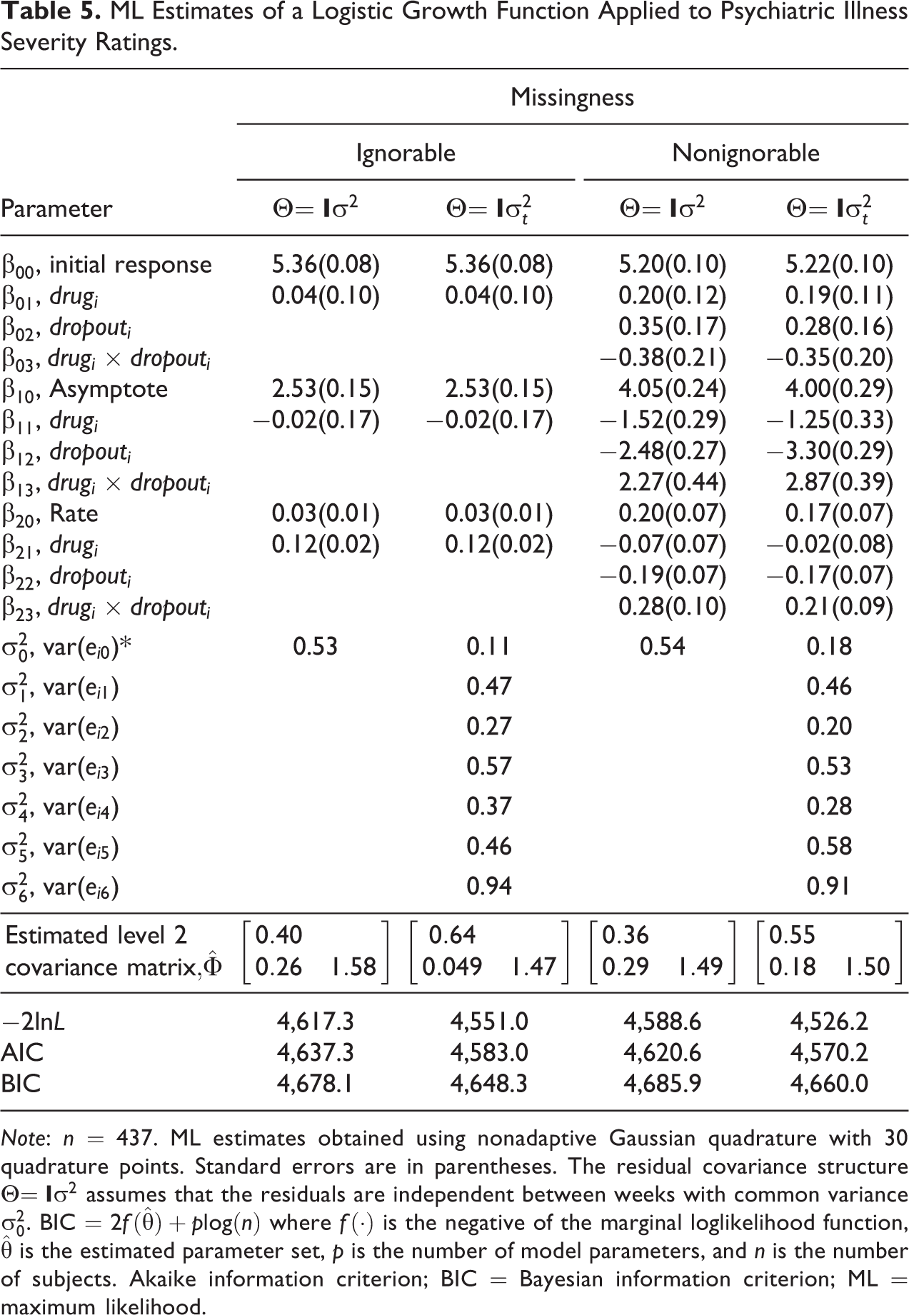
Note: n = 437. ML estimates obtained using nonadaptive Gaussian quadrature with 30 quadrature points. Standard errors are in parentheses. The residual covariance structure
Assuming different residual covariance structures, as well as assumptions about missingness, the estimated variances of the random intercept and asymptote differed. Generally, the estimated variances of the random intercept
Discussion
Considering alternative residual structures at the first level of a mixed-effects model that is linear in its parameters is made straightforward using major statistical software programs such as SAS and SPSS. The need for covariance structures as alternatives to the standard structure that assumes the residuals are independent with constant variance to improve model fit and provide more appropriate parameter estimates has been documented in several studies (Chi and Reinsel 1989; Ferron et al. 2002; Kwok et al. 2007; Sivo et al. 2005). Options for fitting alternative residual covariance structures for nonlinear mixed-effects models are limited for commercial software and require some effort to modify standard syntax for estimation of these models (Harring and Blozis 2014). Thus, applications of models that make use of residual covariance structures that differ from the standard assumption of independence and homogeneity of variance are rare, and understanding the impact of relaxing the standard assumption about the residuals is therefore not well understood. Based on the empirical examples presented in this article, considering alternative residuals structures for a nonlinear mixed-effects model can be an important element in the process of model assessment and inference, particularly given that nonlinear mixed-effects models are much more complex than those in the family of linear mixed-effects models.
The first example presented in this article was based on learning data. In the example, model fit was improved by allowing for dependencies in the level 1 residuals by using a first-order autoregressive structure, a finding that suggested some dependency between scores even after fitting subject-specific growth curves. A consequence of allowing for dependencies in the residuals resulted in an increased estimate of the random intercept and a decreased estimate of the random asymptote using ML estimation. Conversely, both of the estimated variances decreased using Bayes estimation. Only the latter result using Bayes estimation is consistent to what others have described for linear mixed-effects models. Chi and Reinsel (1989), for example, describe how the random effects of a growth model may serve to account for a serial correlation between measures within person and that this serial correlation may be better represented at the first level of the model so as to not inflate the importance of a random effect. Chi and Reinsel’s work relied on ML for estimation of the linear mixed-effects models although here the estimates resulting from Bayesian estimation produced results that were consistent with this earlier work. Here, ML produced results inconsistent with these other patterns, a finding that suggests a sensitivity of the variance estimator to both the assumptions about the covariance structure and estimation procedure.
The second example presented in this article illustrated the impact of considering alternative residual structures for longitudinal measures of illness severity for a patient population and for which data were incomplete and the missingness possibly not ignorable. In the example provided, assumptions about the residual covariance structure had its most notable impact on a model that assumed nonignorable missingness. Although conclusions about missingness for the patient data reported here is, in general, consistent with other studies that suggest that missingness is not likely to be ignorable (see Hedeker and Gibbons 1997), the particular conclusions about the patterns of missing data were driven in part by the assumptions that were made about the residual covariance structure. Such a finding suggests possible implications of fitting alternative residual covariance structures in the understanding of the mechanisms that give rise to missing data.
The work presented here represents one aspect of the process of evaluating model fit for longitudinal data, with a focus on nonlinear mixed-effects models. Certainly, the issue of model specification for longitudinal data more generally can present a great challenge to researchers. Although our focus and that of others concerns mixed-effects model and latent growth models, and in particular, the need to consider alternative residual covariance structures at the first level of a model, a higher level challenge is in selecting a model that will provide a framework for testing hypotheses and providing a good representation of the data (Liu, Rovine, and Molenaar 2012). Added to these issues is the need to address features of the data, such as data that are not measured at the same time points for individuals. Also relevant to the estimation of longitudinal models is the potential increase in the difficulty of estimation, particularly as models become increasingly complex. Estimation of nonlinear mixed-effects models is indeed complex relative to linear models. Estimation of such models that also require more complex specifications of the residual covariance structure can potentially increase computational demand. Increased model complexity can also reduce the precision of parameter estimates. Although these can be unfortunate consequences of considering more complex models, the ultimate goal is to provide a reasonable representation of the data. Considering different residual covariance structures, whether a growth model is linear or nonlinear in its parameters, can yield information in the more general process of evaluating longitudinal models.
As a final note, results from the present investigation suggest some sensitivity of parameter estimates to choices in estimation, namely, ML and Bayes. Based on an analysis of learning data provided here, discrepancies between ML and Bayes lead to different interpretations. In particular, a first-order autoregressive structure was needed to describe the data (similar to the problems considered for linear mixed-effects models in the extant literature). As discussed, the estimated variance of the random intercept increased under ML, whereas it decreased under Bayes, after allowing for the autocorrelation. This pattern resulting from the Bayes estimates is consistent with findings from linear models, but results from ML were inconsistent with previous research. Although certainly beyond the scope of this article, this finding suggests a need for future work to understand the role of estimation choices in fitting such complex models.
Supplemental Material
Supplemental Material, Appendices_Blozis_Harring - Fitting Nonlinear Mixed-effects Models With Alternative Residual Covariance Structures
Supplemental Material, Appendices_Blozis_Harring for Fitting Nonlinear Mixed-effects Models With Alternative Residual Covariance Structures by Shelley A. Blozis and Jeffrey R. Harring in Sociological Methods & Research
Footnotes
Declaration of Conflicting Interests
The author(s) declared no potential conflicts of interest with respect to the research, authorship, and/or publication of this article.
Funding
The author(s) received no financial support for the research, authorship, and/or publication of this article.
Supplemental Material
Supplemental material for this article is available online.
Note
References
Supplementary Material
Please find the following supplemental material available below.
For Open Access articles published under a Creative Commons License, all supplemental material carries the same license as the article it is associated with.
For non-Open Access articles published, all supplemental material carries a non-exclusive license, and permission requests for re-use of supplemental material or any part of supplemental material shall be sent directly to the copyright owner as specified in the copyright notice associated with the article.