Interactions in Fixed Effects Regression Models

Abstract

An interaction in a fixed effects (FE) regression is usually specified by demeaning the product term. However, algebraic transformations reveal that this strategy does not yield a within-unit estimator. Instead, the standard FE interaction estimator reflects unit-level differences of the interacted variables. This property allows interactions of a time-constant variable and a time-varying variable in FE to be estimated but may yield unwanted results if both variables vary within units. In such cases, Monte Carlo experiments confirm that the standard FE estimator of x ⋅ z is biased if x is correlated with an unobserved unit-specific moderator of z (or vice versa). A within estimator of an interaction can be obtained by first demeaning each variable and then demeaning their product. This “double-demeaned” estimator is not subject to bias caused by unobserved effect heterogeneity. It is, however, less efficient than standard FE and only works with T > 2.

Keywords

panel data fixed effects interaction within estimator quadratic terms nonlinearities double demeaning FEIS

Introduction

Fixed effects (FE) regressions are routinely employed by empirical social scientists, especially when analyzing panel data¹ (see, e.g., Young and Johnson 2015). Formally, the FE estimator is defined by an ordinary least squares (OLS) estimation on unit-mean centered data. The main reason for the popularity of this estimator is its potential to improve causal interpretations (Gangl 2010; Morgan and Winship 2007): FE estimation is based solely on variation within units, so it automatically controls for all observable and unobservable unit-specific characteristics (Allison 2009; Wooldridge 2010).

Many scholars have addressed the analytical properties of the FE estimator (e.g., Baltagi 2005; Brüderl and Ludwig 2015; Cameron and Trivedi 2005), dealt with different approaches to its specification in regression frameworks (Andreß, Golsch, and Schmidt 2013; Firebaugh, Warner, and Massoglia 2013; Mundlak 1978), its theory-into-practice problems (Halaby 2004, Giesselmann and Windzio 2014; Plümper, Troeger, and Manow 2005), and its inferential problems (Bell, Fairbrother, and Jones 2018). Here, we focus on an issue that has not yet been addressed in great detail: the specification of interactions in an FE regression. Specifically, we focus on the interaction of two time-varying variables, such as number of children and income - as modeled by Kühhirt (2012) to explain variations in couples’ division of labor.

Basically, an interaction measures how the effect of an independent variable changes with the size of another, moderator variable. In ordinary regression frameworks, an interaction is usually specified by including the product of the original variables (Allison 1977; Jaccardi and Turrisi 2003):

y_{i t} = β_{0} + β_{x} x_{i t} + β_{z} z_{i t} + β_{z x} (z_{i t} x_{i t}) + w_{i t} .

In equation (1), $β_{z x}$ measures the interaction between x and z; $β_{x}$ and $β_{z}$ measure main effects at reference values of z and x; and $w_{i t}$ is the error term, which may include both unit-specific and time-specific components. The standard way of specifying an interaction in FE is to treat the interaction term as any other variable and, accordingly, to demean it: Each realization of the product is subtracted by its unit-specific mean before entering the regression:

y_{i t} - {\bar{y}}_{i .} = β_{x} (x_{i t} - {\bar{x}}_{i .}) + β_{z} (z_{i t} - {\bar{z}}_{i .}) + β_{z x} (z_{i t} x_{i t} - {\bar{(z x)}}_{i .}) + w_{i t (f e)} .

This specification for interactions in FE is widely used in empirical practice (e.g., Killewald and Gough 2013; Schofer and Longhofer 2011) and is usually referred to as within estimation (e.g., Abendroth, Huffman and Treas 2014; Kühhirt 2012; Oesch and Lipps 2013). It is also computed by default by statistical programs (Cameron and Trivedi 2009), introduced as a desirable specification in methodological discourses (Schunck 2013), and numerically equivalent to an OLS interaction estimation with unit dummies.

However, this strategy does not yield a within estimator of the interaction: The estimator of $β_{z x}$ in equation (2) uses between-unit differences in the effects of z, x, or both z and x; it will include effect heterogeneity. This is contrary to the common view that “[f]ixed effects estimates […] use only within-individual differences, essentially discarding any information about differences between individuals” (Allison 2009, p. 3; see also Brüderl and Ludwig 2015; Halaby 2004). They do so for the estimators of main effects but not for interactions. Hence, interactions estimated with standard FE are subject to bias caused by unobserved heterogeneity as Figure 1 illustrates: For both graphs (A) and (B),² the effect of x on y is influenced by two variables: time-varying z1, which is included, and time-constant z2, which is not included. In Figure 1A, but not in Figure 1B, standard FE will yield an unbiased interaction estimator for $β_{z 1 x}$ . Thus, the standard FE interaction estimator (hereafter FE-IE) assumes that included moderators and time-constant unobserved moderators of a variable are not correlated. If this assumption holds, standard FE can be used to estimate an interaction; if it does not, one might consider specifying an alternative, strict within-unit interaction estimator.

Figure 1.

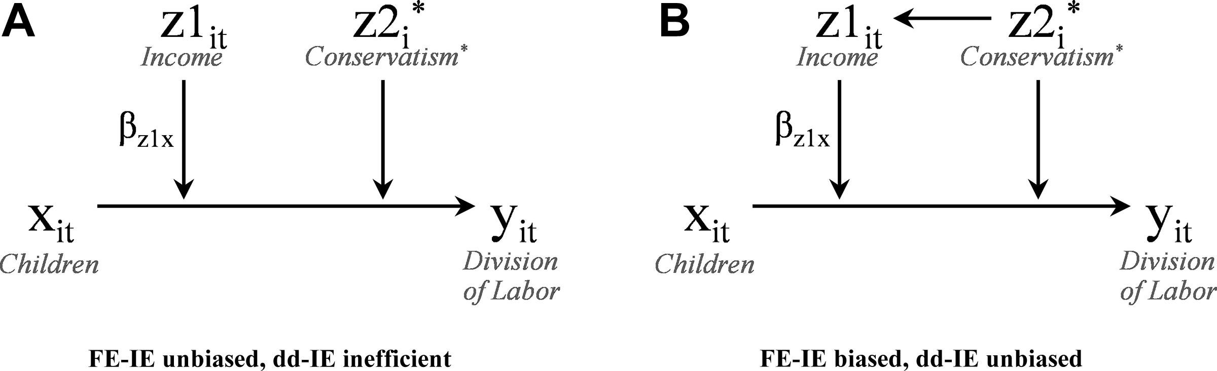
Two graphs in which an unobserved time-constant moderator z2 (A) does not or (B) does influence an included moderator z1 (practical example in italics).

For example, when the interaction between income and having children on couples’ division of labor is modeled (Kühhirt 2012), FE-IE not only measures how changes in income within households influence the effect of having children. It also measures how this effect differs between households with different (average) income levels. It therefore includes the moderating influence of income-correlated time-constant unobservables (e.g., traditionalism, conservatism) on the effect of having children. Therefore, the model’s FE interaction estimates assume that such unit-specific unobservables either do not moderate the effect of having children or are uncorrelated with income. If neither of these conditions holds, as illustrated in Figure 1B, the standard FE interaction estimator will be biased.

In what follows, we formally prove these properties of FE-IE and discuss an alternative: the double-demeaned interaction estimator (hereafter dd-IE). This is a strict within-unit interaction estimator that does not rely on the assumption of uncorrelated unit-specific moderators (and therefore is unbiased for both graphs in Figure 1).

The Algebra of the FE-IE

A within estimator of an interaction between z and x on y measures how the within-unit effect of x is related to within-unit variation in a moderator z. The integration of the demeaned interaction term $z_{i t} x_{i t} - {\bar{(z x)}}_{i .}$ in an FE regression framework, as outlined in equation (2), yields an estimator of $β_{z x}$ that is still identifiable when one of the two variables exhibits only between-unit variance. Thus, the most straightforward demonstration that FE-IE uses between-unit differences in effects to determine the interaction is that a unit-specific characteristic (i.e., a variable that is constant within units) can be estimated as a moderator of a time-varying variable x in FE.

This property arises from a basic arithmetic feature of demeaned products: The higher the unit-specific mean of one factor, the more strongly are the idiosyncrasies of the other factor accentuated in the factors’ demeaned products. Thus, the unit-specific variance of demeaned products depends on the unit-specific levels of z and x. Hence, demeaned products follow a distribution that reflects both the idiosyncrasies and the unit-specific levels of the interacted variables. This arithmetic feature allows us to differentiate within-unit effects across categories (or levels) of time-constant variables in FE regressions. Therefore, incorporating the demeaned product of a time-constant variable and a time-varying variable into an FE regression is a standard procedure in panel data analysis. However, this arithmetic feature also defines FE-IE as a between estimator if both interacted variables show within-unit variation.

To support these insights formally, we show how demeaned products unfold algebraically in standard FE interactions.

For any measurement ${i, t}$ , the demeaned interaction term $z_{i t} x_{i t} - {\bar{(z x)}}_{i .}$ in equation (2) can be written as

z_{i t} x_{i t} - \frac{\sum_{t = 1}^{T_{i}} z_{i t} x_{i t}}{T_{i}},

with every $z_{i t}$ and $x_{i t}$ consisting of a unit-specific component - ${\bar{z}}_{i .}$ and ${\bar{x}}_{i .}$ - and a measurement-specific component - $(z_{i t} - {\bar{z}}_{i .})$ and $(x_{i t} - {\bar{x}}_{i .}$ ), which we will write as ${\ddot{z}}_{i t}$ and ${\ddot{x}}_{i t}$ from here.

Now let us consider three constellations of z and x: (a) Neither variable shows within-unit variation, (b) only one variable shows within-unit variation, and (c) both variables show within-unit variation. How does the demeaned interaction term in equation (3) unfold algebraically in these cases and what does this reveal about the properties of FE-IE in each constellation?

Neither Variable Shows Within-unit Variation

If both variables are time constant, then $x_{i t} = {\bar{x}}_{i .}$ and $z_{i t} = {\bar{z}}_{i .}$ for each ${i, t}$ . Therefore, we can rewrite equation (3) as

{\bar{z}}_{i .} {\bar{x}}_{i .} - \frac{T_{i} ({\bar{z}}_{i .} {\bar{x}}_{i .})}{T_{i}},

which is zero for each ${i, t}$ . Thus, demeaning an interaction term with two unit-specific, time-constant variables eliminates all between-unit variation from both variables, so no moderating influence of z on the effect of x can be identified.

Only One Variable Shows Within-unit Variation

If, x varies and z is constant within units, then $z_{i t} = {\bar{z}}_{i .}$ for all ${i, t}$ and the demeaned interaction term from equation (3) can be written as

{\bar{z}}_{i .} x_{i t} - \frac{\sum_{t = 1}^{T_{i}} {\bar{z}}_{i .} x_{i t}}{T_{i}} .

For each measurement ${i, t}$ , ${\bar{z}}_{i .}$ is a factor in all added terms in the subtrahend of equation (5), which therefore can be transformed to³

{\bar{z}}_{i .} {\ddot{x}}_{i t} .

Thus, if x shows within-unit variation and z does not, their demeaned product measures between-unit differences of z and within-unit differences of x. FE-IE in this case estimates how the within-unit effect of x differs according to between-unit levels of z. As noted, this is nothing new and is a characteristic of FE that is widely used in empirical practice. It is mostly considered desirable because it allows FE estimation of interactions between time-constant and time-varying variables. Thus, demeaning the product term is generally a useful strategy if the interaction of one time-constant variable and one time-varying variable is analyzed with an FE regression, even though (or rather because) it does not yield a strict within estimator.

Both Variables Show Within-unit Variation

We have seen that two time-constant variables are completely eliminated in a demeaned interaction term. However, as soon as one variable shows within-unit variation, the unit-specific component of the other variable is reflected in their demeaned product. Therefore, if both variables vary within units, FE-IE will be identified from variance in the unit-specific levels of both variables.

To demonstrate this more formally, we rewrite the demeaned interaction term from equation (3) as

({\bar{z}}_{i .} + {\ddot{z}}_{i t}) ({\bar{x}}_{i .} + {\overset{}{\ddot{x}}}_{i t}) - \frac{\sum_{t = 1}^{T_{i}} ({\bar{z}}_{i .} + {\overset{}{\ddot{z}}}_{i t}) ({\bar{x}}_{i .} + {\overset{}{\ddot{x}}}_{i t})}{T_{i}} .

Using fractional arithmetic, as shown in Appendix A2 (which can be found at http://smr.sagepub.com/supplemental/), equation (7) can be transformed to

{\bar{z}}_{i .} {\overset{}{\ddot{x}}}_{i t} + {\bar{x}}_{i .} {\overset{}{\ddot{z}}}_{i t} + {\overset{}{\ddot{z}}}_{i t} {\overset{}{\ddot{x}}}_{i t} - \frac{\sum_{t = 1}^{T_{i}} {\overset{}{\ddot{z}}}_{i t} {\overset{}{\ddot{x}}}_{i t}}{T_{i}},

which reveals that, for each measurement ${i, t}$ , a demeaned product of two time-varying variables z and x includes unit-specific levels of both z and x. More specifically, we see that the size of the demeaned interaction term depends on the products of (a) the unit-specific mean in z and the demeaned value of x, of (b) the unit-specific mean in x and the demeaned value of z, and of (c) both demeaned values of x and z. Thus, for two time-varying variables, FE-IE in equation (2) measures a combination of

the moderating influence of between-unit differences in z on the within-unit effect of x,

the moderating influence of between-unit differences in x on the within-unit effect of z, and

the moderating influence of within-unit differences in z on the within-unit effect of x.

Hence, FE-IE not only measures how the within-unit effect of x on y changes with within-unit variation of z, it also reflects the moderating property of the unit-specific level of z on the within-unit effect of x, and vice versa. This means that it does not control for correlated effect heterogeneity in x and z across units—which explains algebraically why Balli and Sørensen (2013) find standard FE interactions to be biased in the presence of unobservable unit effect heterogeneity. Thus, FE-IE hinges on the assumption that within-unit variation of z influences the effect of x in the same way as does between-unit variation of z (and vice versa).

Formally, these conclusions rest on the persistence of unit-specific effect heterogeneity in the FE error term: If the model outlined in equation (1) includes effect heterogeneity and therefore

w_{i t} = u_{0 i} + u_{1 i} x_{i t} + e_{i t},

then, as shown in Appendix A3 (which can be found at http://smr.sagepub.com/supplemental/), the error term of the FE-transformed model in equation (2) also includes effect heterogeneity:

w_{i t (f e)} = u_{1 i} {\overset{}{\ddot{x}}}_{i t} + e_{i t} .

Thus, if a correlated unobserved time-constant moderator exists, such that $u_{1 i}$ is correlated with $z_{i t}$ , then $u_{1 i} {\overset{}{\ddot{x}}}_{i t}$ , the first component of the decomposed FE error term in equation (10), is correlated with ${\bar{z}}_{i .} {\overset{}{\ddot{x}}}_{i t}$ , the first component of the decomposed FE interaction term in equation (8). Therefore, as illustrated in Figure 1B, FE-IE in this case will be biased.

A Within Estimator of Interactions: dd-IE

If standard FE does not provide a strict within estimator of the interaction between two time-varying variables, how can we obtain one? In this case, rather than the demeaned product of two variables, we may specify the product of two demeaned variables, as in

{\overset{}{\ddot{y}}}_{i t} = β_{x} {\overset{}{\ddot{x}}}_{i t} + β_{z} {\overset{}{\ddot{z}}}_{i t} + β_{z x} {\overset{}{\ddot{z}}}_{i t} {\overset{}{\ddot{x}}}_{i t} + w_{i t (f e)} .

This strategy eliminates unit heterogeneity in the basic elements of the interaction, the factors. The term ${\overset{}{\ddot{z}}}_{i t} {\overset{}{\ddot{x}}}_{i t}$ relates within-unit idiosyncrasies of x to within-unit idiosyncrasies of z. Consequently, the estimator of $β_{z x}$ in equation (11) measures how the within-unit association between x and y changes with within-unit variation of z. Therefore, it does not rely on the assumption that unit-specific effect heterogeneity in x is uncorrelated with z. If, due to time-constant moderators, $u_{1 i}$ in the FE error term $w_{i t (f e)}$ in equation (10) is correlated with moderator $z_{i t}$ , the components of the interaction term in equation (11) are not: Demeaned variables are generically orthogonal to any unit-specific component.

Yet this strategy presents a problem: The demeaned product of two time-varying variables does not have a unit-specific mean value of zero unless the two variables are perfectly uncorrelated. Instead, the unit-specific mean of ${\overset{}{\ddot{z}}}_{i t} {\overset{}{\ddot{x}}}_{i t}$ depends on the unit-specific degree of intraindividual correlation between x and z. Therefore, if an unobserved moderator is related to ${Corr}_{i} (x, z)$ , its effect will be transported in the estimator of $β_{z x}$ in equation (11). To eliminate all between-unit heterogeneity from interaction effect estimation, the product of the demeaned variables must again be demeaned. Then, we arrive at a specification that is functionally equivalent to a specification introduced by Balli and Sørensen (2013):

{\overset{}{\ddot{y}}}_{i t} = β_{x} {\overset{}{\ddot{x}}}_{i t} + β_{z} {\overset{}{\ddot{z}}}_{i t} + β_{z x} {\overset{}{\ddot{z}}}_{i t} {\overset{}{\ddot{x}}}_{i t} - {\bar{{\overset{}{\ddot{z}}}_{i t} {\overset{}{\ddot{x}}}_{i t}}}_{i .} + w_{i t (f e)},

where the double-demeaned interaction ${\overset{}{\ddot{z}}}_{i t} {\overset{}{\ddot{x}}}_{i t} - {\bar{{\overset{}{\ddot{z}}}_{i t} {\overset{}{\ddot{x}}}_{i t}}}_{i .}$ can be written either as

(z_{i t} - {\bar{z}}_{i .}) (x_{i t} - {\bar{x}}_{i .}) - {\bar{(z_{i t} - {\bar{z}}_{i .}) (x_{i t} - {\bar{x}}_{i .})}}_{i .},

or as

{(\ddot{{\ddot{z}}_{i t} {\ddot{x}}_{i t}})}_{i .} .

This term describes a complete within-unit transformation of an interaction: As in equation (11), unit-specific means are fully eliminated from the factors. Therefore, their product is orthogonalized to all unit-specific components in the FE error term $w_{i t (f e)}$ in equation (from 10). Additionally, the products’ mean value within each unit is now fixed at zero, so that heterogeneity in levels, effects, and covariances is eliminated. Therefore, the estimator of $β_{z x}$ in equation (12), the double-demeaned FE-interaction estimator (dd-IE), is unbiased in the presence of correlated time-constant unobserved moderators, as Figure 1 illustrates.

However, compared with the standard FE interaction estimator (FE-IE), a substantial proportion of the variance in the interaction term is eliminated by using dd-IE. Thus, the cost of reducing bias is less efficient estimates. These two statistical properties of dd-IE, being less prone to bias but less efficient as well, are also emphasized by the Monte Carlo experiments detailed in the next section.

Simulations of Various FE Interaction Specification

Simulation Setup

We simulated data using the following basic data-generating process (DGP):

y_{i t} = β_{0} + β_{x} x_{i t} + β_{z 1} z 1_{i t} + β_{z 1 x} z 1_{i t} x_{i t} + β_{z 2} z 2_{i t} + β_{z 2 x} z 2_{i t} x_{i t} + u_{i} + e_{i t},

where $β_{0} = 0, β_{x} = β_{z 1} = β_{z 2} = 1$ and $β_{z 1 x} = - 1$ .⁴

In this DGP, $β_{z 2 x}$ varies across conditions, as will be explained further below. This data-generating model is a standard unobserved effects model with three variables in its fixed part: x, z1, and z2. Each of these variables consists of a unit-specific component (x_i , $z 1_{i}$ , and $z 2_{i}$ ), varying only between units i, and a within-unit component varying within units over time ( ${\overset{}{\ddot{x}}}_{i t}$ , ${\ddot{z 1}}_{i t}$ , and ${\ddot{z 2}}_{i t}$ ).⁵ Thus,

x_{i t} = x_{i} + {\overset{}{\ddot{x}}}_{i t},

z 1_{i t} = z 1_{i} + {\ddot{z 1}}_{i t},

z 2_{i t} = z 2_{i} + {\ddot{z 2}}_{i t} .

All these components and the unit-specific and the idiosyncratic error terms (u_i and e_it ) are drawn from a joint multivariate standard normal distribution; they have a mean of 0 and a standard deviation of 1, except for the error terms, which have a standard deviation of 4. The error terms are uncorrelated with each other and with all other variables in the model. The correlations among the variables x, z1, and z2 vary across conditions as explained below.

The DGP contains two interactions with the variable x, one with z1 and another one with z2. The variable z1 represents an observed variable, whereas z2 represents an unobserved variable. Thus, the effect of the variable x is moderated by an observed moderator, z1, and an unobserved moderator, z2. Accordingly, the models fitted to the generated data use only the variables x and z1, whereas z2 (and its interaction) is omitted.

What varies are three parameters from the DGP in equation (15):

The effects of β _z _2x. The coefficient β _z _2x takes the values 0, −0.5, and −1. If it takes the value 0, there is no unobserved moderation of the effect of x. For β _z _2x = −0.5, the unobserved moderator effect is half as strong as the observed effect, and for β _z _2x = −1, it is of the same strength.

The correlations between the observed and the unobserved unit-specific components z1 _i and z2 _i . The correlation Corr(z1 _i , z2 _i ) takes the values 0, 0.4, 0.8, representing nonexistent, moderate, and strong correlations.

The correlations between the observed and unobserved within-unit components ${\ddot{z 1}}_{i} and {\ddot{z 2}}_{i}$ . The correlation Corr( ${\ddot{z 1}}_{i}$ , ${\ddot{z 2}}_{i}$ ) also takes the values 0, 0.4, and 0.8, again representing nonexistent, moderate, and fairly strong correlations. Note that if Corr( ${\ddot{z 1}}_{i}$ , ${\ddot{z 2}}_{i}$ ) = 0, only the time-constant component of z2 is correlated with z1. Therefore, this scenario is analog to a scenario in which the unobserved correlated moderator z2 is time constant.

For each combination of these conditions, we generate data based on the DGP and fit a model to it using the standard FE transformation, obtaining FE-IE as in equation (2), and a model in which the variables are first demeaned then interacted and then demeaned again, thus obtaining dd-IE as in equation (12). For each combination of conditions, we simulate a population with 1,000,000 observations consisting of 100,000 units, each observed 10 times. From these populations, we draw 1,000 samples, to which we fit the two models. Each sample consists of 100 units and 1,000 observations with 10 observations per unit.

In an additional simulation, we further vary the number of observations T per unit. T takes the values 3, 10, and 30. To this additional condition, we fit an estimator as in equation (11), where the two interacting variables are first demeaned, then multiplied but not demeaned again, and then compare it with dd-IE from equation (12). The purpose of these additional simulations is to show that it is necessary to demean the product of two demeaned variables to obtain an unbiased estimator.

Results: FE-IE and dd-IE

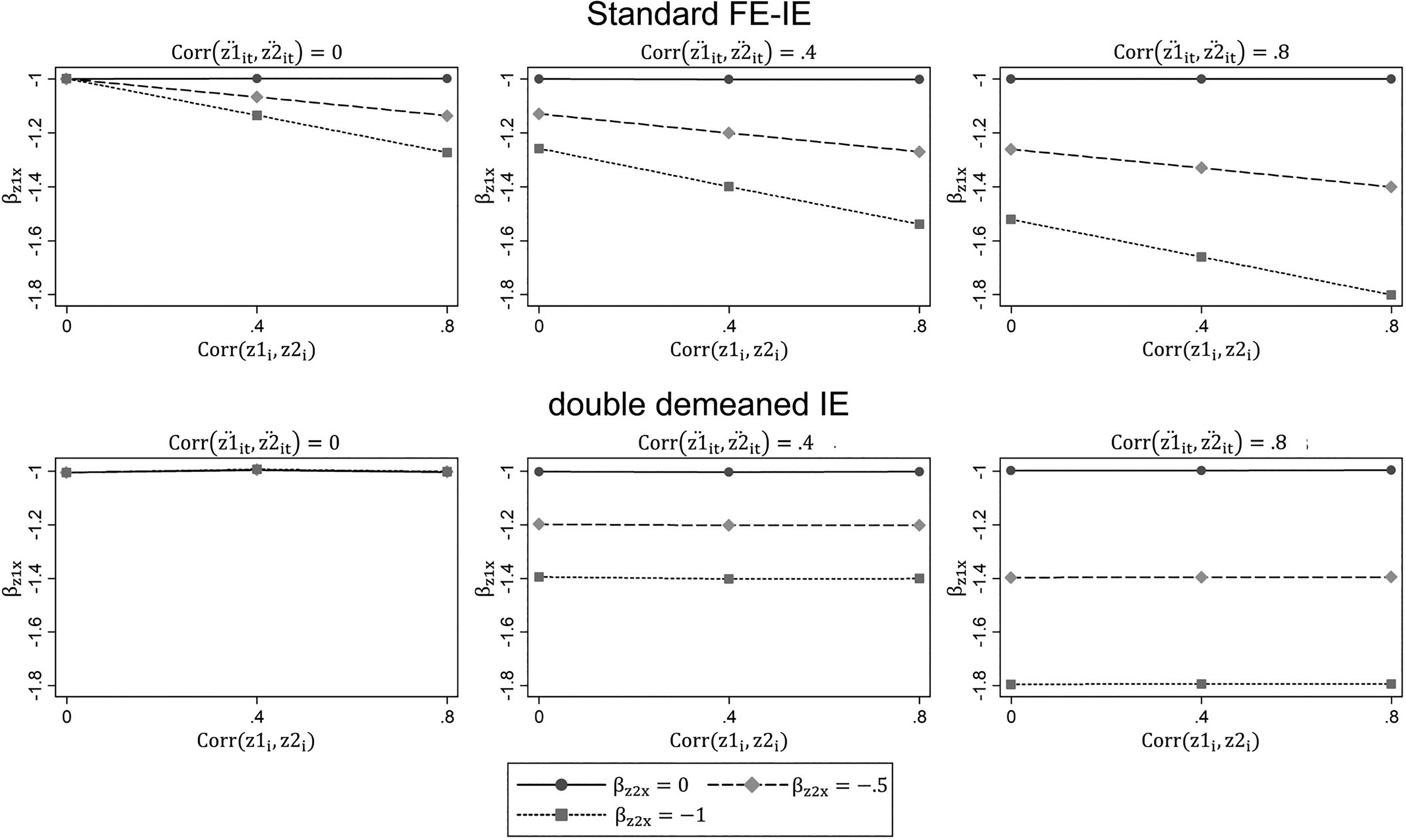
Figure 2 shows the results of the simulation study. We present only the estimated interaction effect β _z _1x. The top panel in Figure 2 shows FE-IE, and the bottom panel shows dd-IE. The correlation between the within-unit components of the included and the omitted moderator, ${\ddot{z 1}}_{i t}$ and ${\ddot{z 2}}_{i t}$ , varies over the columns of Figure 2. The x-axes of the single graphs show the correlation between the unit-specific components of $z 1_{i}$ and $z 2_{i}$ . The y-axes give the average of the estimated effect β _z _1x, where the true effect equals −1. Finally, each graph contains three lines representing the different true values of β _z _2x; the different strengths of the unobserved interaction effect.

Figure 2.

Average interaction estimates by conditions (1,000 simulations per condition).

As the upper panel of Figure 2 shows, FE-IE gives an unbiased estimate of the interaction between x and z1 under two conditions: (a) if there is no interaction between x and the omitted moderator z2 ( $β_{z 2 x} = 0$ , the solid line in each graph of the upper panel) and (b) if the omitted moderator variable z2 is not correlated with the included moderator z1 (the very left of the left graph in the upper panel, where the within-unit and the unit-specific components of z1 and z2 are uncorrelated). If there is an unobserved interaction between x and z2 ( $β_{z 2 x} \neq 0$ ) and z1 and z2 are correlated, FE-IE is biased because it carries part of the unobserved interaction effect. In this setting, there is a negative bias because the unobserved interaction effect is negative and the correlation between the two moderators z1 and z2 is positive. This bias increases both with the correlation of unit-specific components $Corr (z 1_{i}, z 2_{i})$ and the correlation of within-unit components $Corr ({\ddot{z 1}}_{i t}, {\ddot{z 2}}_{i t})$ .

In contrast, dd-IE (bottom panel of Figure 2) is not biased if the correlation between the included moderator z1 and the omitted moderator z2 originates solely from the between-unit components of these variables (left graph in the bottom panel). This implies that the dd-IE automatically controls for an omitted interaction with a time-constant variable, which by definition can have only between-unit covariation with the variables in the model. If the correlation between z1 and z2 originates from the within-unit components of these variables (middle and right graph of the bottom panel), the estimator will also be biased, just like FE-IE: dd-IE controls for correlated effect heterogeneity across units; it does not control for interactions of correlated unobserved time-varying variables.

The unbiasedness of dd-IE under conditions in which FE-IE is biased comes at a price: FE-IE is more efficient than dd-IE. In our setting, the standard deviation of the estimated coefficients (the empirical standard error [SE]) from the 1,000 samplings is about twice as high for dd-IE as for FE-IE. More precisely, on average, over all conditions, the standard deviation is 2.61 times larger for dd-IE when compared with FE-IE (min = 1.30, max = 4.04).⁶ However, the loss of efficiency depends on the degree of variance that is eliminated by the double-demeaning procedure, as opposed to a single demeaning as in the FE-IE. We did not vary this parameter but used fixed variance components in our simulation setup. A perhaps realistic picture of the loss of statistical power to be expected when using dd-IE in empirical research is offered by our replication results below.

Omitting the Second Demeaning: Why Not Make It Simpler?

Finally, we compare the statistical properties of dd-IE with an estimator received from including the product of two demeaned variables as in equation (11) but not demeaning this product again. In the simulations depicted in Figure 3, we estimate such models with varying numbers of observations T per unit. To keep the comparison simple, we do not vary any other parameter. 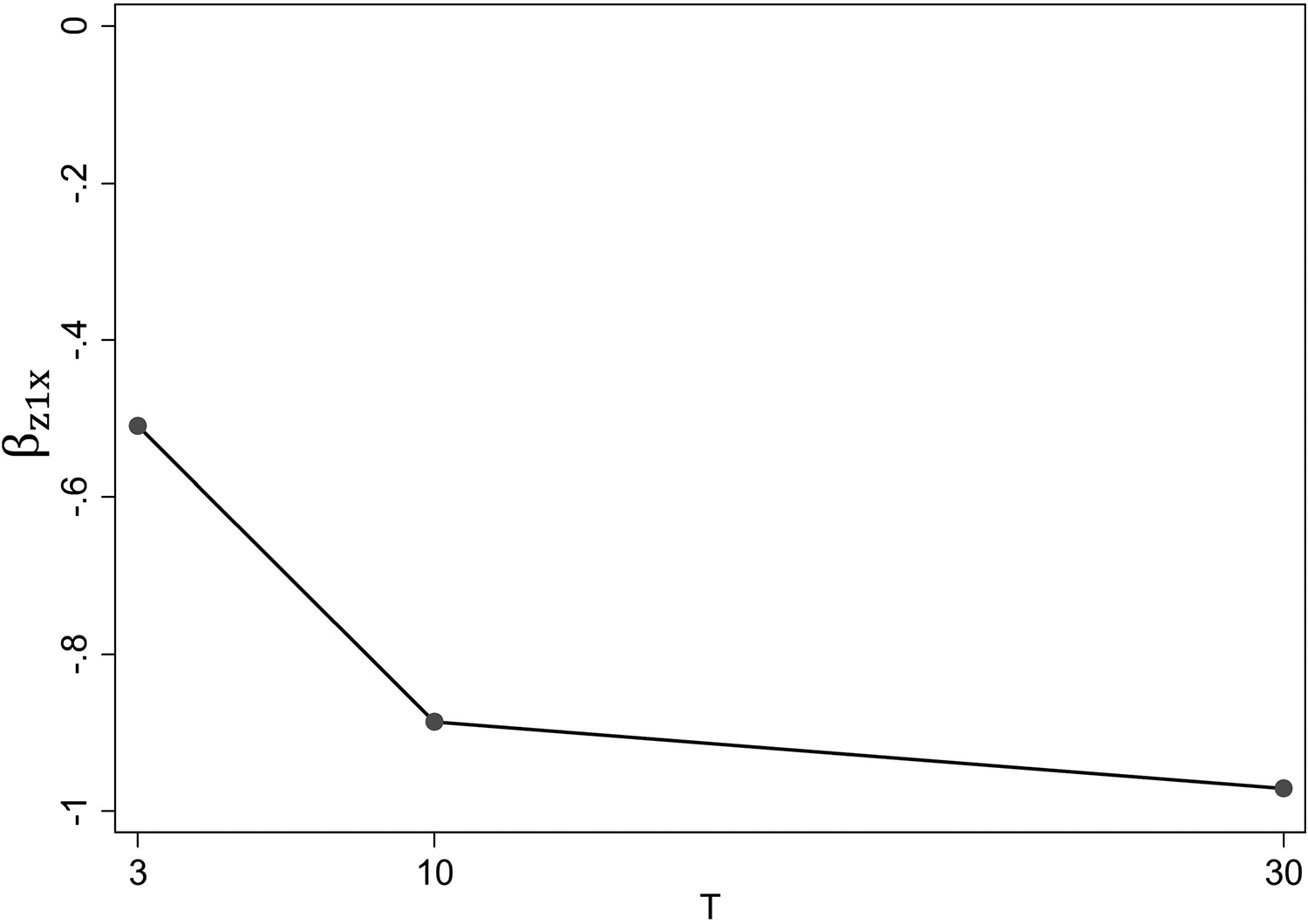We consider only the scenario where $Corr (z 1_{i}, z 2_{i})$ and $Corr ({\ddot{z 1}}_{i t}, {\ddot{z 2}}_{i t})$ equal 0 and the population parameter $β_{z 2 x}$ equals $- 1$ ; this is a scenario in which both FE-IE and dd-IE gave unbiased results.⁷

Figure 3.

Effect of varying T on estimator without second demeaning.

The estimate without the second demeaning is biased even if the included moderator z1 is not correlated with the omitted moderator z2. The bias diminishes in size with an increasing number of observations per unit. It occurs because the unit-specific mean value of a term obtained by multiplying two demeaned variables is not necessarily zero, even if the idiosyncrasies of the interacted variables are not correlated (and therefore $Corr ({\ddot{z 1}}_{i t}, {\ddot{z 2}}_{i t}) = 0$ ): The smaller the number of observations per unit, the more the unit-specific means of the interaction term ${\ddot{z 1}}_{i t} {\ddot{z 2}}_{i t}$ deviate from zero by chance. This adds random variance to the realizations of the interaction term, thus evoking a bias toward zero, similar to what has been termed attenuation bias (also known as regression dilution), which occurs because of random measurement errors in the independent variables (Frost and Thompson 2000; Spearman 1904). Note that dd-IE in Figure 2 does not show this kind of bias because an additional demeaning of the product will eliminate the random variance in unit-level differences.

In addition to the bias toward zero, there may be a systematic bias in an estimator that suppresses the second demeaning. This can be the case if the product of the two demeaned variables differs systematically from zero (see above). Additional simulations, which are not presented here, indicate that such systematic bias occurs when the strength of the intraindividual correlation of z1 and x is correlated with z2. Compared with the bias toward zero, however, this systematic bias appears to be of minor importance.

In sum, our additional simulations show that the term ${\ddot{z 1}}_{i t}$ ${\ddot{z 2}}_{i t}$ does indeed need to be demeaned. The estimator without the second demeaning is subject to a bias toward zero owing to random variation in its mean. It can also be subject to unobserved variable bias if the correlation between ${\ddot{z 1}}_{i t}$ and ${\ddot{z 2}}_{i t}$ depends on the level of an unobserved effect.

dd-IE in Practice

The previous sections introduced the double-demeaned interaction estimator (dd-IE) as an alternative to the standard FE estimator of an interaction (FE-IE). In this section, we discuss some practical considerations.

Practical Implementation

The practical implementation of dd-IE is straightforward: First, (a) the interacted variables are demeaned, and (b) the product of the demeaned variables is generated. Next, (c) this product and all covariates are demeaned and finally (d) included as explanatory variables in a regression analysis on a demeaned dependent variable. Statistical software usually provides commands that automatically process steps (b), (c), and (d). Thus, the first demeaning, (a), has to be done manually.

In the Online Appendix to this article, we provide a syntax for Stata that integrates all four steps (Appendix A4, which can be found at http://smr.sagepub.com/supplemental/). This syntax illustrates the practical implementation of dd-IE on the basis of a replication of Schunck (2013), but it can also be used as a blueprint for other analyses. The code is based on the xtreg, fe command but adds the first demeaning of the interacted variables.

Whenever interaction effects are estimated, coefficients of main effects must be interpreted with care, because a variable’s estimated main effect always refers to the zero point of its moderator. Thus, in a standard FE model, estimates of main effects refer to the value of zero of their moderators. However, with unit-mean centered factors, estimates of the variables’ main effects refer to the means of their moderators. Thus, to harmonize the reference points for main effects between FE-IE and dd-IE, the syntax also contains a command that grand-mean centers the variables before any demeaning. In such a specification, the factors’ main effects in the standard FE model also refer to the means of their moderators.

Double Demeaning or Standard FEs?

As we have shown, the standard FE estimate of an interaction is biased as soon as an unobserved time-constant moderator of the interacted variable is correlated with the included moderator of the same variable. By contrast, dd-IE is not prone to bearing the moderating effect of unobserved heterogeneity. However, the elimination of effect heterogeneity from the interaction comes at a price: a loss of efficiency, as illustrated by our Monte Carlo experiments above and the replications below. This is not surprising given that FE-IE uses between-unit variation in the effects of the independent variables to construct the interaction coefficient, as shown in equation (8), whereas dd-IE discards this source of variance.

Which of the two estimators is to be preferred in a research scenario with two time-varying interacted variables? This question can be linked to a general methodological debate about the trade-off between the consistency and efficiency of within estimators. While some authors state that “throwing out between variation is not wasting data” (Halaby 2004, p. 52) and advocate a strict use of within estimators in causal analysis (see also Brüderl and Ludwig 2015), other authors explicitly justify the use of between-unit variation in the absence of time-constant unobservable confounders (Allison 2009; Wooldridge 2010).

From the latter perspective, the choice between FE-IE and dd-IE depends on assumptions about the properties of time-constant, unobservable moderators. If effect heterogeneity in x and z exists, a standard assumption in hierarchical modeling, and the underlying unobserved moderators are assumed to be correlated with one of the interacted variables, as illustrated in Figure 1B, the FE-IE of the interaction $x \cdot z$ is biased, but dd-IE is not. The latter then seems to be the better choice. In contrast, if the assumption is justified that unobservable time-constant moderators of x are not correlated with z, and those of z not with x, FE-IE would be the better choice (see Figure 1A). To give an example: when using standard FE to estimate the interaction effect between marriage and having children, Killewald and Gough (2013) implicitly assume that time-constant unobservables correlated with marriage (e.g., emotional stability, locus of control) do not moderate the effect of having children on income. If they considered an interaction between such unit-specific unobservables and having children to be plausible, dd-IE might well be a more suitable modeling strategy than FE-IE.

An empirical criterion that can be employed to decide between FE-IE and dd-IE is the Hausman (1978) test. This technique has been established as standard for testing an efficient but possibly biased estimator against an unbiased but less efficient estimator (Wooldridge 2010). It is often used in longitudinal analyses to decide between RE and FE for main effects (Allison 2009) and can easily be adapted to test against the null hypothesis that standard FE estimates of an interaction are identical to double-demeaned estimates. The syntax provided in the Appendix shows a straightforward implementation of this adapted test in Stata.

In addition to theoretical and formal considerations, there are some caveats that researchers should consider before using dd-IE (or other strategies to control for effect heterogeneity). One is that even regular interaction estimators often tend to be statistically underpowered (Aguinies 1995), and this problem is exacerbated through double demeaning. A more specific caveat is that the variance of two observations per unit does not suffice to identify the coefficient of a factor of two centered variables, as shown formally in the Online Appendix (A5, [1]–[4], http://smr.sagepub.com/supplemental/). Thus, in order to apply dd-IE, panel data are needed from at least three waves. In unbalanced panels, only units with more than two measures contribute to dd-IE. Hence, researchers might cautiously report standard FE coefficients of interactions even in cases where the assumption of no correlated time-constant moderators is problematic, specifically in low-T scenarios.

SEs

Although the multiplication of unit-mean-centered variables yields a constant term at the unit level for T = 2, this identification restriction is not accompanied by any additional loss of degrees of freedom (DF): A third observation allows two demeaned products to vary freely. We confirmed this in additional simulations: In the absence of any dependency in the DGP’s residual, the empirical SE of dd-IE is predicted correctly by the normal FE deduction of 1 DF per unit, while subtracting 2 DF leads to overly conservative estimates of variability (results available on request). Therefore, whenever the regular SE estimation for FE-IE seems appropriate, it can also be used for dd-IE.

FEs With Individual Slopes (FEIS): An Alternative Within-unit Interaction Estimator?

An alternative way to control for time-constant unobserved moderators in FE is the integration of unit-specific slopes (FEIS) for interacted variables. Instead of eliminating between-unit variance in moderators’ effects through double demeaning, FEIS swaps out unit-specific effect heterogeneity through its systematic specification: by integrating individual slopes for x and z in equation (2), u _1i $\begin{array}{l} {\ddot{x}}_{i t} \end{array}$ (and u _2i $\begin{array}{l} {\ddot{z}}_{i t} \end{array}$ ) from the error term in equation (10) are shifted to the fixed part of the FE model.

Evidently, when applied in large-N situations, this technique is computationally challenging. Furthermore, it demands more degrees of freedom than double demeaning, as two additional parameters are fixed per unit. While Wooldridge (2010) and Brüderl and Ludwig (2015) discuss solutions to the first problem (which blossomed into the Stata ado xtfeis), the second issue results in differing properties in FEIS and dd-IE: In FEIS, time-constant variables can no longer be identified as moderators of variables with individual slopes, which is possible using dd-IE. Furthermore, unlike double demeaning, the FEIS solution does not work with T = 3: Unless heterogeneity in levels is left unfixed and essentially OLS-IS is specified, FEIS with slopes for both interacted variables omits all units with less than four measures from the interaction estimate.

Given these properties, dd-IE appears to be the more efficient strategy for estimating a within-unit interaction, especially in scenarios with many units and few observations per unit, which is typical for longitudinal microdata. However, the complete elimination of effect heterogeneity from the FE error term through FEIS is accompanied by inferential benefits (see e.g., Bell et al. 2018). These may outweigh the advantages of dd-IE over FEIS for interaction estimation, especially in large-T situations.⁸

Combining both dd-IE and FEIS in a model is a practical solution for person fixed-effects models with additional time effects or, more generally, in two-way FE models. Assume we had another unobserved moderator of x in Figure 1, z3, which is constant within measures at similar time points, such as family policy configuration, and also correlated with z1. Then, adding individual slopes for time dummies to a model with person-level dd-IE controls for both person-specific and time-specific effect heterogeneity correlated with z1.

Replications

In the Introduction section, we referred to several studies that use standard FE to test interactions of time-varying variables (Abendroth et al. 2014; Killewald and Gough 2013; Kühhirt 2012; Oesch and Lipps 2013; Schofer and Longhofer 2011; Schunck 2013). These studies explicitly aim at within estimation, were published in highly ranked sociological journals, and have had considerable impact as indicated by strong citation records. To examine the practical relevance of our insights into FE interactions, we conducted replications of these studies.

For this purpose, we contacted the six corresponding authors, five of whom replied and sent us their syntax files. We retrieved the data needed for the replications from infrastructure organizations under regulations of public or scientific use.⁹ Because of the strict policy on the protection of data from the European Community Household Panel (ECHP), we refrained from replicating Abendroth et al.’s (2014) analyses. Eventually, we replicated analyses from four studies. We first identified the models that are related to the main interaction hypotheses. We then reproduced the original results which are based on FE-IE. Next, we used dd-IE. To obtain estimates of main effects on a comparable scale, the data were grand-mean centered before estimation.

Where possible, we performed a Hausman test to identify systematic differences between FE-IE and dd-IE. Two of the studies computed separate models for women and men, so in total, we conducted six analyses. All analyses were done using Stata Version 14.1 (StataCorp 2015). Our basic replication strategy is documented in Appendix A4 (which can be found at http://smr.sagepub.com/supplemental/). Table 1 gives an overview of the key parameters and results of the replications. Here, we focus only on the interaction of interest, whereas Tables A6(1) to A6(6) in the Appendix present all coefficients of the original and replicated models. As indicated in the Table’s notes, the published results and our replicated results of the standard FE models differ slightly in some cases. In these cases, we reported the results from our replication so as to provide an appropriate reference for comparison with dd-IE.

Table 1.

The Estimation of Interactions Through Standard Fixed Effects and Double Demeaning: Replications of Published Analyses.

Replication Model	1		2		3		4		5		6
Study	Schunck (2013)^a		Oesch and Lipps (2013) ^b				Kühhirt (2012) ^c		Killewald and Gough (2013) ^d
Data
Sample	Mothers (United States)		Adult women (Germany)		Adult men (Germany)		Partnered men (Germany)		Adult men (United States)		Adult women (United States)
Source	NCHS		SOEP V.27		SOEP V.27		SOEP V.31		NLSY79		NLSY79
Period	1990–1998		1984–2010		1984–2010		1984–2007		1979–2008		1979–2008
Total observations (n)	8,604		126,925		144,261		12,872		56,403		46,240
N (with t > 1)	3,978		11,730		14,148		1,527		4,411		3,915
N (with t > 2)	648		10,361		12,426		1,331		4,308		3,805
Variables
Dependent variable	Birth weight (child)		Life satisfaction (0–10)		Life satisfaction (0–10)		Childcare (daily time in hours)		Hourly wage (logged)		Hourly wage (logged)
Interactor X	Smoking (y/n)		Unemployment (y/n)		Unemployment (y/n)		2+ Children in household (y/n)		Having 2+ children (y/n)		Having 2+ children (y/n)
Interactor Z	Age (mother)		Regional unemployment rate		Regional unemployment rate		Logged HH income		Married (y/n)		Married (y/n)
	B	SE	B	SE	B	SE	B	SE	B	SE	B	SE
Replication with standard FE (original results)
FE-IE	3.79	4.96	−0.017***	0.003	0.006*	0.003	−0.43***	0.088	0.082***	0.017	−0.016	0.021
Replications with double-demeaned estimator
dd-IE	−78.98^†	46.81	−0.006	0.01	−0.03**	0.01	−0.02	0.13	−0.032	0.022	−0.057*	0.028
Hausman test: FE-IE vs. dd-IE	p = .52		(χ² < 0)		p = .018		p = .017		—		—

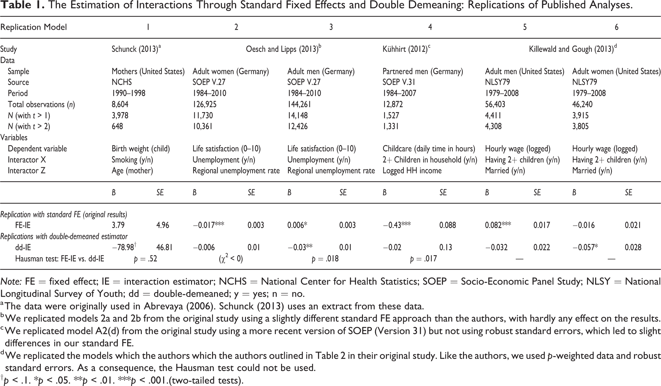
Note: FE = fixed effect; IE = interaction estimator; NCHS = National Center for Health Statistics; SOEP = Socio-Economic Panel Study; NLSY = National Longitudinal Survey of Youth; dd = double-demeaned; y = yes; n = no.

^a The data were originally used in Abrevaya (2006). Schunck (2013) uses an extract from these data.

^b We replicated models 2a and 2b from the original study using a slightly different standard FE approach than the authors, with hardly any effect on the results.

^c We replicated model A2(d) from the original study using a more recent version of SOEP (Version 31) but not using robust standard errors, which led to slight differences in our standard FE.

^d We replicated the models which the authors which the authors outlined in Table 2 in their original study. Like the authors, we used p-weighted data and robust standard errors. As a consequence, the Hausman test could not be used.

^† p < .1. *p < .05. **p < .01. ***p < .001.(two-tailed tests).

The study by Schunck (2013) is didactically motivated, uses training data, and estimates how the effect of a mother’s age on an infant’s birth weight is moderated by smoking. FE-IE (3.97) is substantively but not statistically different from dd-IE (−79.98). For the latter, the SE increases enormously as a result of the data structure: Of the overall sample of 3,978 mothers, only 648 provide more than two observations. Of these, less than 10 percent show variation in smoking. Consequently, only 54 mothers are used to identify the dd-IE.

The study by Oesch and Lipps (2013) tests how individual unemployment influences the effect of ambient unemployment on life satisfaction. While the influence of unobserved time-constant characteristics (e.g., empathy, locus of control) on the effect of ambient unemployment are controlled for in the dd-IE, they are not controlled for in the standard FE model used by the authors. Indeed, for men, FE-IE (0.0006*) differs significantly from dd-IE (−0.030**): Using only within-unit variation, individual unemployment is no longer estimated to mitigate but to accentuate the negative impact of ambient unemployment on life satisfaction. For women, the finding that individual unemployment accentuates the negative effect of ambient unemployment on life satisfaction (FE-IE: −0.017***) is no longer statistically significant using dd-IE (−0.006).¹⁰ Although a majority of individuals in the sample provide more than two measures, the decrease in precision due to double demeaning is substantial: SEs are nearly 4 times higher than in FE-IE, probably as a result of weak intraindividual variation in ambient unemployment over time.

Kühhirt’s (2012) analysis is concerned with the impact of income on the effect of the number of children on a man’s daily time in childcare. The standard FE coefficient of the interaction between having additional children and logged income is significantly negative (−0.43***), while dd-IE is significantly larger and close to zero (−0.02). When only within-unit variation is used to estimate the interaction, the conclusion that household income decreases the impact of additional children on men’s involvement in childcare is no longer supported. The SEs do not increase substantively by double demeaning. We assume this is due to the high proportion of intraindividual variation in logged income and number of children.¹¹

Finally, the study by Killewald and Gough (2013) examines whether marital status influences the parenthood wage premium. For males, the standard FEs estimation reported by the authors provides a positive interaction between marriage and having more than one child on logged wage (0.082***). This is interpreted as evidence that marriage increases the fatherhood wage premium. However, FE-IE uses differences in the parenthood effect between constantly married and unmarried men. Therefore, it is prone to include the moderating effects on parenthood of time-constant characteristics correlated with marriage (e.g., emotional stability). By contrast, dd-IE focuses on the group of men with changing marital status, comparing their parenthood effects in periods when they were married with periods when they were not. Using dd-IE, the interaction switches its sign and becomes insignificant (−0.032). Because probability-weighted data and robust SEs were used, a Hausman test on this difference cannot be performed in Stata.¹² Still, dd-IE weakens evidence for a marriage-related increase of the fatherhood wage premium. It also provides stronger support for the specialization hypothesis for women: While FE-IE for women is close to zero (−0.016), dd-IE yields a significant negative interaction between marital status and motherhood (2+ children) on logged wage (0.057*), indicating an increased wage penalty of motherhood through marriage.

All of the replicated studies reveal differences between FE-IE and dd-IE. For two models (3 and 4), the Hausman test indicated statistically significant differences; for one model (1), it did not find any systematic differences; and for three models (2, 5, and 6), it could not be applied. However, for one of these three models (5), the interaction estimate switches from significantly positive to negative. Thus, at least three of the six replicated FE-IEs are likely to include the moderating effects of omitted correlated time-constant variables. If an estimator were used that has the statistical properties expected by the authors, conclusions would differ in these cases. At the same time, all SEs obtained with dd-IE are higher than with FE-IE. The growth ranges between factors 1.3 (Replication Model 6) and 25.3 (Replication Model 1) depending on the longitudinal structure of the data and the degree of within-unit variation in the interacted variables.

Discussion

By using empirical considerations, formal arguments, and Monte Carlo experiments, we have shown that the standard approach to specifying an FE interaction, demeaning the product term (FE-IE), does not yield a strict within estimator. Instead, FE-IE measures a combination of several between-unit and within-unit interdependencies as shown in equation (8). It includes the moderating influence of unit-specific characteristics that are omitted as moderators and correlated with the interacted variables. Therefore, the standard FEs estimator of x·z is biased if z is influenced by an unobserved unit-specific moderator of the effect of x, or vice versa. In contrast, first demeaning the factors and then demeaning the product, double demeaning, eliminates unit-specific elements from the interaction term completely. Consequently, this double-demeaned interaction estimator dd-IE is a strict within-unit estimator and therefore yields more consistent results in the presence of correlated unit-specific unobserved or omitted moderators.

However, dd-IE is less efficient than FE-IE. It yields imprecise estimates if the interacted variables’ within-unit variation is small or the number of measures per unit is low. Moreover, it only works for interactions of time-varying variables and requires more than two measures per unit. The same is true for alternative within-unit interaction estimators, as fixed effects with individual slopes (FEIS) for both interacted variables. Such problems are well known from methodological discourses on within estimators (e.g., Allison 2009, p. 23), but they appear to be more severe with interactions, particularly due to the omission of all units with T < 3 from dd-IE (and T < 4 from FEIS for both interacted variables).

As standard FE works fine for interactions if there is no correlated unobserved time-constant moderator, one may conclude that double demeaning should not be conducted by default but only where necessary: If there is significant theoretical or empirical evidence for unobservable, unit-specific moderators with influence on the included moderator. Conversely, one might argue that collecting and using panel data is based on the idea that correlated unobserved heterogeneity generally exists in nonexperimental research. Therefore, an assumption that prefers FE-IE may be regarded as inconsistent with the usual motivation behind using panel data (see also Halaby 2004). From this perspective, it would be more consistent to use dd-IE by default.

Besides using strict within-unit interaction estimators, our formal considerations suggest another strategy to circumvent the problems of standard FE interactions: the suppression of within-unit variation in one of the two interacted variables, as empirically demonstrated by Schober and Stahl (2016). To examine an interaction of two time-varying variables in an FE regression of life satisfaction, these authors used the person mean (averaged over years) of day care availability as moderator of maternal employment. Clearly, this strategy does not yield a strict within-unit interaction estimator. However, according to transformations outlined in equation (5) and equation (6), suppressing within-unit variation in one moderator provides the moderated strict within-unit effect of the other interacted variable.¹³ Thus, unlike FE-IE, which measures a mix of within-unit and between-unit interactions, the estimator of $\ddot{\bar{x} z}$ allows a clear and technically consistent interpretation; for instance, Schober and Stahl (2016) use it to measure how the within-person effect of maternal employment on life satisfaction varies between settings with different average levels of day care provision. Obviously, this strategy is adequate if theory allows a unit-specific moderator. However, it may also provide an alternative if low degrees of within-unit variation in one interacted variable (or a small-T situation) do not permit dd-IE.

Independent of the perspective on within versus between estimation, our contribution can be read as support for scholars to increase transparency in reporting the properties and assumptions of their FE-IEs. It may also encourage the inclusion of interactions with observable time-constant covariates, following the insights that their moderating properties on time-varying variables are not automatically controlled in standard FE models. As our review of studies shows, FE-IE is usually misleadingly introduced as a within estimator and credited with corresponding statistical properties. Schofer and Longhofer (2011), for example, measure the effects of policy indicators on the number of occupational associations. They introduce their estimator as exploiting only “within-case variability over time” (p. 559); as shown, this is not correct for the standard FE coefficient of the interaction between degree of democracy and state expansion reported in the study. Similarly, Abendroth et al. (2014) assert that their FE model on determinants of mothers’ occupational status “provide stringent tests of within-person change” (p. 10). However, their hypothesis that mothers’ age influences the effect of higher order births was tested by FE-IE and is therefore not based solely on within-unit variation.

The same goes for Oesch and Lipps (2013) who emphasize that their “fixed effects model […] exploits only within-unit variance” (p. 959). Actually, it also picks up differences in the effect of ambient unemployment on life satisfaction between individuals with different employment status—and therefore relies on the assumption that unobserved time-constant moderators of ambient unemployment have no influence on employment status. Killewald and Gough (2013) state that their FEs models “control for selection into family forms that is correlated with fixed but unobserved individual traits that are also correlated with wages” (p. 483). However, this is not true for the interaction they report; their FE-IE measures the influence of marriage on the effect of having children not only within but also between individuals, meaning that it is prone to include moderating influences on the effect of having children of those time-constant variables that influence selection into marriage.

Finally, we would like to emphasize that a quadratic variable can be regarded as a special case of interaction. Therefore, the mechanisms presented in this article also apply to FE estimation of squared variables: Demeaning the product of a quadratic term in an FE framework will yield a coefficient β _xx that includes the unit-specific moderating influences of this variable, as shown in equation (8); it will use unit-specific differences of x to estimate its nonlinear relationship with y.¹⁴ To obtain a within estimator of a quadratic term, the variable must similarly be demeaned before being transformed into its nonlinear form.

Supplemental Material

Supplemental Material, 2a_Appendix_Table_r3 - Interactions in Fixed Effects Regression Models

Supplemental Material, 2a_Appendix_Table_r3 for Interactions in Fixed Effects Regression Models by Marco Giesselmann and Alexander W. Schmidt-Catran in Sociological Methods & Research

Supplemental Material

Supplemental Material, 2_Appendix_Main_R3 - Interactions in Fixed Effects Regression Models

Supplemental Material, 2_Appendix_Main_R3 for Interactions in Fixed Effects Regression Models by Marco Giesselmann and Alexander W. Schmidt-Catran in Sociological Methods & Research

Footnotes

Acknowledgment

We are grateful for feedback from members of the section “Methods of Empirical Social Research” of the German Sociological Association, specifically at the 38th DGS Congress in Bamberg. We thank Conrad Ziller for pointing us to the identification problem in small-T situations. Furthermore, comments from two anonymous reviewers, Hans-Jürgen Andress, David Brady, Pat Hastings, Tabea Naujoks, Simon Milligan and Pia Schober were extremely helpful. We are grateful that Alexandra Killewald, Michael Kühhirt, Oliver Lipps, and Reinhard Schunck shared their code and provided helpful hints for our replications of their studies. Marco Giesselmann also thanks Heinz Althoff and Günther Wehmeyer for elementary insights and support.

Declaration of Conflicting Interests

The author(s) declared no potential conflicts of interest with respect to the research, authorship, and/or publication of this article.

Funding

The author(s) received no financial support for the research, authorship, and/or publication of this article.

ORCID iD

Marco Giesselmann

Supplemental Material

Supplemental material for this article is available online.

Notes

References

Abendroth

Anja-Kristin

Huffman

Matt L.

Treas

Judith

. 2014. “The Parity Penalty in Life Course Perspective: Motherhood and Occupational Status in 13 European Countries.” American Sociological Review 79:993–1014.

Abrevaya

Jason

. 2006. “Estimating the Effect of Smoking on Birth Outcomes Using a Matched Panel Data Approach.” Journal of Applied Econometrics 21:489–519.

Aguinies

Herman

. 1995. “Statistical Power with Moderated Multiple Regression in Management Research.” Journal of Management 21:1141–58.

Allison

Paul D.

1977. “Testing for Interaction in Multiple Regression.” American Journal of Sociology 83:144–53.

Allison

Paul D.

2009. Fixed Effects Regression Models. Los Angeles: Sage.

Andreß

Hans-Jürgen

Golsch

Katrin

Schmidt

Alexander W.

. 2013. Applied Panel Data Analysis for Economic and Social Surveys. Berlin, Germany: Springer.

Balli

Hatice O.

Sørensen

Bent E.

. 2013. “Interaction Effects in Econometrics.” Empirical Economics 45:583–603.

Baltagi

Badi H.

2005. Econometric Analysis of Panel Data. Chichester, England: Wiley.

Bell

Andrew

Fairbrother

Malcolm

Jones

Kelvyn

. 2018. “Fixed and Random Effects Models: Making an Informed Choice” Quality & Quantity 55:117.

10.

Brüderl

Josef

Ludwig

Volker

. 2015. “Fixed-effects Panel Regression.” Pp. 327–57 in The Sage Handbook of Regression Analysis and Causal Inference, edited by Best

Wolf

. Los Angeles, CA: Sage.

11.

Bureau of Labor Statistics, U.S. Department of Labor. 2008. National Longitudinal Survey of Youth 1979 Cohort. Columbus: Center for Human Resource Research, The Ohio State University.

12.

Cameron

A. Colin

Trivedi

Pravin K.

. 2005. Microeconometrics: Methods and Applications. New York: Cambridge University Press.

13.

Cameron

A. Colin

Trivedi

Pravin K.

. 2009. Microeconometrics Using Stata. College Station, TX: Stata Press.

14.

Firebaugh

Glenn

Warner

Cody

Massoglia

Michael

. 2013. “Fixed Effects, Random Effects, and Hybrid Models for Causal Analysis.” Pp. 113–32 in Handbook of Causal Analysis for Social Research, edited by Morgan

S. L.

. Dordrecht, the Netherlands: Springer Science + Business.

15.

Frost

Chris

Thompson

Simon G.

. 2000. “Correcting for Regression Dilution Bias: Comparison of Methods for a Single Predictor Variable.” Journal of the Royal Statistical Society: Series A (Statistics in Society) 163:173–89.

16.

Gangl

Markus

. 2010. “Causal Inference in Sociological Research.” Annual Review of Sociology 36:21–47.

17.

Giesselmann

Marco

Windzio

Michael

. 2014. “Paneldaten in der Soziologie: Fixed Effects Paradigma und empirische Praxis in Panelregression und Ereignisanalyse.” Kölner Zeitschrift für Soziologie und Sozialpsychologie 66:95–114.

18.

Giesselmann

Marco

Bohmann

Sandra

Goebel

Jan

Krause

Peter

Liebau

Elisabeth

Richter

David

Schacht

Diana

Schröder

Carsten

Schupp

Jürgen

Liebig

Stefan

. 2019. “The Individual in Context(s): Research Potentials of the Socio-Economic Panel Study (SOEP) in Sociology.” European Sociological Review 35:738–55.

19.

Halaby

Charles N.

2004. “Panel Models in Sociological Research: Theory into Practice.” Annual Review of Sociology 30:507–44.

20.

Hausman

Jerry A.

1978. “Specification Tests in Econometrics.” Econometrica 46:1251-71.

21.

Jaccard

James

Turrisi

Robert

. 2003. Interaction Effects in Multiple Regression, 2nd ed. Thousand Oaks, CA: Sage.

22.

Killewald

Alexandra

Gough

Margaret

. 2013. “Does Specialization Explain Marriage Penalties and Premiums?” American Sociological Review 78:477–502.

23.

Knight

Carly R.

Christopher

Winship

. 2013. “The Causal Implications of Mechanistic Thinking: Identification Using Directed Acyclic Graphs (DAGs).” Pp. 275–99 in Handbook of Causal Analysis for Social Research, edited by Morgan

S. L.

. Dordrecht, the Netherlands: Springer.

24.

Kühhirt

Michael

. 2012. “Childbirth and the Long-term Division of Labour Within Couples: How Do Substitution, Bargaining Power, and Norms Affect Parents’ Time Allocation in West Germany?” European Sociological Review 28:565–82.

25.

McIntosh

Craig T.

Schlenker

Wolfram

. 2006. Identifying Non-linearities In Fixed Effects Models. San Diego: School of Global Policy & Strategy, University of California. Retrieved October 12, 2016 (https://gps.ucsd.edu/_files/faculty/mcintosh/mcintosh_research_identifying.pdf).

26.

Morgan

Stephen L.

Winship

Christopher

. 2007. Counterfactuals and Causal Inference: Methods and Principles for Social Research. New York: Cambridge University Press.

27.

Mundlak

Yair

. 1978. “On the Pooling of Time Series and Cross Section Data.” Econometrica 46:69–85.

28.

Oesch

Daniel

Lipps

Oliver

. 2013. “Does Unemployment Hurt Less If There Is More of It Around? A Panel Analysis of Life Satisfaction in Germany and Switzerland.” European Sociological Review 29:955–67.

29.

Plümper

Thomas

Troeger

Vera E.

Manow

. 2005. “Panel Data Analysis in Comparative Politics: Linking Method to Theory.” European Journal of Political Research 44:327–54.

30.

Schober

Pia S.

Stahl

Juliane F.

. 2016. “Expansion of Full-day Childcare and Subjective Well-being of Mothers: Interdependencies with Culture and Resources.” European Sociological Review 32:593–606.

31.

Schofer

Evan

Longhofer

Wesley

. 2011. “The Structural Sources of Association.” American Journal of Sociology 117:539–85.

32.

Schunck

Reinhard

. 2013. “Within and Between Estimates in Random-effects Models: Advantages and Drawbacks of Correlated Random Effects and Hybrid Models.” The Stata Journal 13:65–76.

33.

Spearman

Charles

. 1904. “The Proof and Measurement of Association Between Two Things.” The American Journal of Psychology 15:72–101.

34.

StataCorp. 2015. Stata 14 Base Reference Manual. College Station, TX: Stata Press.

35.

Wooldridge

Jeffrey M.

2010. Econometric Analysis of Cross Section and Panel Data, 2nd ed. Cambridge, MA: MIT Press.

36.

Young

Rebekah

Johnson

David R.

. 2015. “Handling Missing Values in Longitudinal Panel Data With Multiple Imputation.” Journal of Marriage and Family 77:277–94.

Supplementary Material

Please find the following supplemental material available below.

For Open Access articles published under a Creative Commons License, all supplemental material carries the same license as the article it is associated with.

For non-Open Access articles published, all supplemental material carries a non-exclusive license, and permission requests for re-use of supplemental material or any part of supplemental material shall be sent directly to the copyright owner as specified in the copyright notice associated with the article.

0.00 MB

0.03 MB

0.12 MB