
Abstract
This contribution deals with effect measures for covariates in ordinal data models to address the interpretation of the results on the extreme categories of the scales, evaluate possible response styles, and motivate collapsing of extreme categories. It provides a simpler interpretation of the influence of the covariates on the probability of the response categories both in standard cumulative link models under the proportional odds assumption and in the recent extension of the Combination of Uncertainty and Preference of the respondents models, the mixture models introduced to account for uncertainty in rating systems. The article shows by means of marginal effect measures that the effects of the covariates are underestimated when the uncertainty component is neglected. Visualization tools for the effect of covariates are proposed, and measures of relative size and partial effect based on rates of change are evaluated by the use of real data sets.
Keywords
Ordinal data models based on a rating procedure are common in different disciplines such as economics, marketing, medicine, and psychology, see, for example, Agresti (2010). Traditional methods for their analysis are generalized linear models that employ nonlinear link functions to cumulative probabilities (McCullagh 1980).
A recent literature deals with an alternative class of models that use a mixture distribution to mimic the decision-making process. More precisely, this class of mixture models considers the selection of a response category as a combination of a deliberate choice based on the preference of the respondent (preference component) and an uncertainty in the process of response (uncertainty component); see Piccolo et al. (2019), Piccolo and Simone (2019), Iannario and Piccolo (2016), Tutz et al. (2017) and reference therein. The preference component accounts for reasoned judgments toward the object/item under evaluation as well as the set of emotions, sentiments, and perceptions logically connected with it. The uncertainty component accounts for other unreasonable elements such as the unconscious willingness to please the interviewer and difficulty in expressing a rating regarding a specific object/item about which the interviewed has not a clear opinion.
In this contribution, we focus on Combination of Uncertainty and Preference of the respondents (
Any model for ordinal data can be used to represent the preference component of a
For the uncertainty component, a uniform distribution is usually envisaged. Nevertheless, other distributions, instead of the Uniform one, maybe considered; supplement learning on this issue is in Gottard et al. (2016), Colombi et al. (2018), and Tutz and Schneider (2019).
In the present article, we focus on the standard
The plan of the article is as follows. In the second section, we discuss the data generating process that motivates the use of
Data Generating Process and CUP Models
Finite mixtures have been advanced by several authors for analyzing ordinal data; see Wedel and DeSarbo (1995), Greene and Hensher (2010), Grün and Leisch (2008), Breen and Luijkx (2010), Iannario and Piccolo (2016), among others. They are generally introduced for improving fitting accuracy, and they are motivated by the development of the data generating process. Finite mixture models for rating data can be broadly classified into two types.
– The models of the first type mimics the behavior of standard mixture models. Respondents can be considered as members of different clusters characterized by alternative rating procedures, each of which is described by a suitable probability distribution. The final mixture is given by a convex combination of these probability distributions.
– The rating assigned by an individual on a specific topic is the final outcome of a complex activity based on knowledge of the topic, instinct, and emotion of the individual. Hence, the mixture can be considered as a combination of the distributions of a discretized version of the underlying continuous latent variables describing these different components. This is the philosophy embraced by the
As previously mentioned,
Original motivations for the selection of the random variables marking out the two components of the
The
Now, we briefly recall the main characteristics of

with
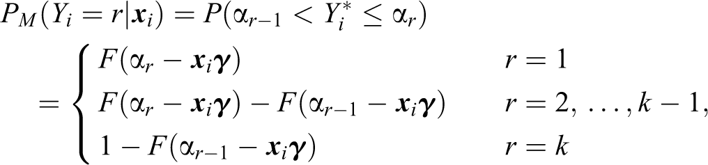
The probability distribution of Yi, that represents the discrete measurement of
The subject propensity to adhere to a well-structured response behavior rather than to a random choice is modeled by mixing the previous components via the uncertainty parameter
In several implementations of
As earlier pointed out and motivated, we describe the preference component of the

where
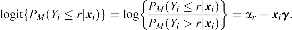
Using the latent variable interpretation of cumulative link models, the preference component can be written as
where
For given
Effect Measures for Covariates in Ordinal Data Models
For
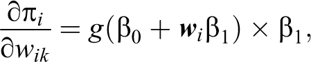
We report below the ME measure of a continuous variable
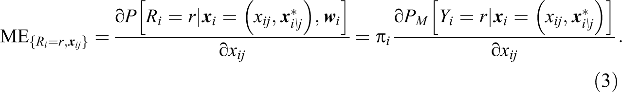
In equation (3), the partial derivative of

where
If

If the number of possible values is greater than two, the discrete change is computed as the difference in the predicted probabilities for cases in one category relative to the reference level.
We now describe how we can obtain the ME of a continuous variable

More in details, we obtain
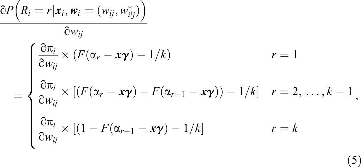
where
and
According to the way we fix the values of the covariates, we can obtain three different types of ME measures.
– The average ME (AME) obtained calculating the mean of the MEs evaluated on the n sample values
– MEs at representative values (MER) obtained calculating the ME for representative values of the covariates (i.e., values of interest in the examined experiment or study).
– MEs at the mean (MEM) obtained by computing the MEs setting all covariates equal to their mean value.
Among these summary measures, Long and Freese (2014) recommended the use of AME since it averages the effects across all cases observed in the sample and thus can be interpreted as the sample average size of the ME. Mood (2010) pointed out that the AME has behavior reminiscent of effects in ordinary linear models, in the sense that it is roughly stable when we add an explanatory variable to the model that is uncorrelated with the variable for which we are describing the effect. This behavior does not occur for the MEM or MER or the log odds ratio. See also Long (1997) and Sun (2015) for a further discussion of the various ME measures. Notice that these measures are denoted in different ways depending on the context (for instance, “elasticity” in econometric literature—see Franses and Paap 2004—or “partial effect” in some statistical fields—see Long 1997). In the following part of the article, unless otherwise specified, we discuss about AME (ME hereafter) measures.
We conclude this section with a motivating example regarding individual perception of working life quality. The source of the data is the “5th European Working Conditions Survey (EWCS)” carried out in 2010 by the European Foundation for the Improvement of Living and Working Conditions (Eurofound). The respondents were asked to express their agreement/disagreement on different aspects of their job. We do not present a comprehensive analysis of the problem, but we only examine respondents’ agreement on
ME Measures for the CUP Model—Eurofound Data.
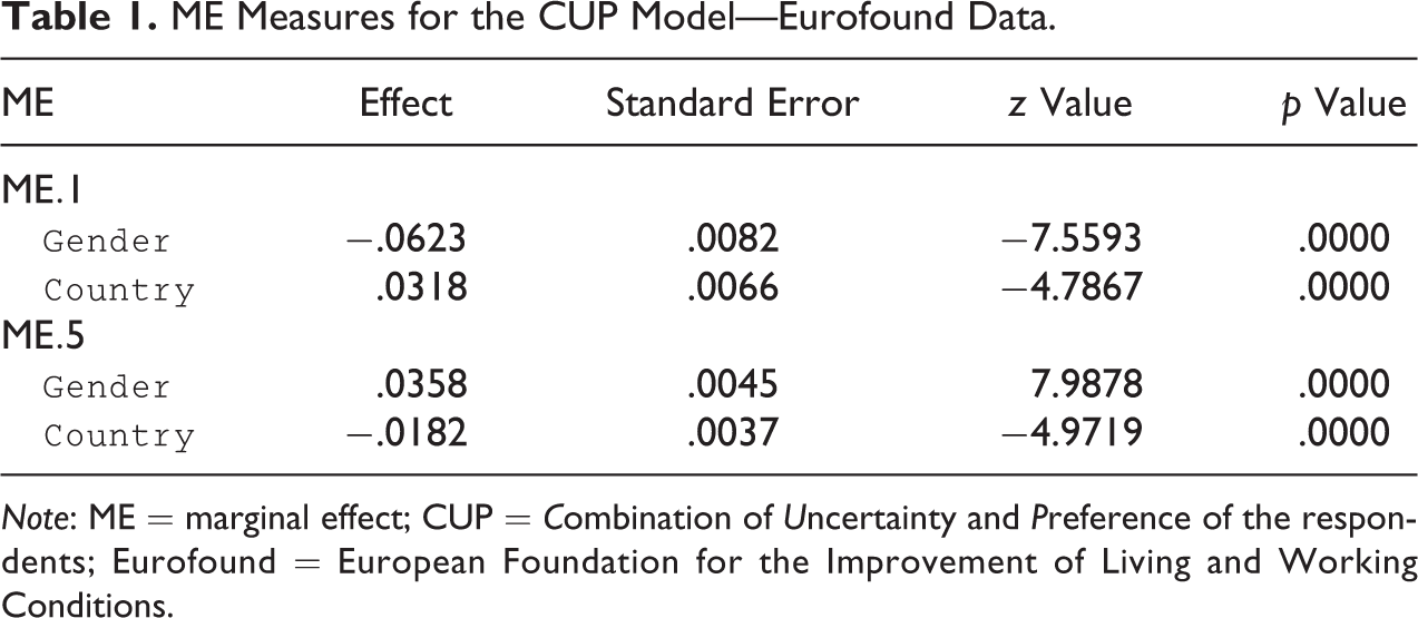
Note: ME = marginal effect; CUP = Combination of Uncertainty and Preference of the respondents; Eurofound = European Foundation for the Improvement of Living and Working Conditions.
Case Studies
In this section, we introduce four case studies to motivate the need of the ME measures proposed in the previous section. The first example underlines the utility of the implementation and the analysis of the ME measures on the extreme categories when the examined model fits poorly for them; the second one shows the possible impact of the uncertainty component on ME measures of the preference one. The third example summarizes the impact of the interaction between covariates improving the main contents of Agresti and Tarantola’s (2018) paper. This example emphasizes as the interaction effects capture the impact of one explanatory variable on the ME measure of another explanatory variable. In fact, while in linear models the effect of a marginal change in the interaction term is equal to the interaction effect, this equality generally does not hold in nonlinear specifications. The last one reports the ME of nominal variables using a well-known data set regarding American presidential elections (Faraway 2006).
Survey of Health, Ageing and Retirement in Europe (SHARE) Data
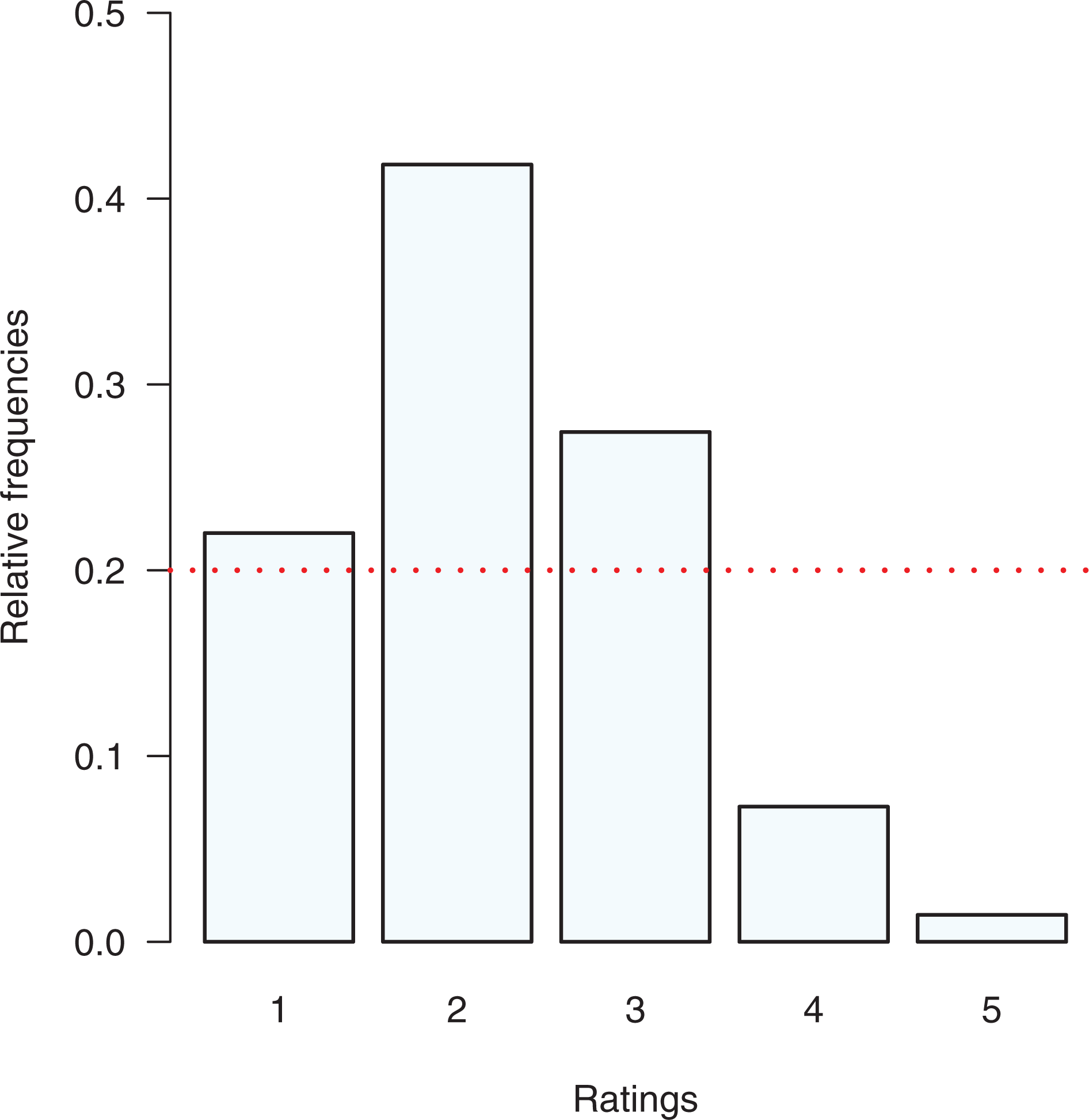
We consider a set of data from wave 1 (2004) of the SHARE. It is a multidisciplinary and cross-national panel database of microdata on health, socioeconomic status, and social and family networks regarding individuals aged 50 or older. It covers 27 European countries and Israel. Up to now, seven survey waves have been collected within the period 2004–2017. The examined survey analyzes how different expectations and attitudes of the 3,458 respondents influence their quality of life. We analyze the rating assigned by the respondents on their pain perception. We use a rating on a five-point Likert-type scale (1 = no pain, 2 = mild, 3 = moderate, 4 = serious, and 5 = severe); covariates introduced for the analysis are
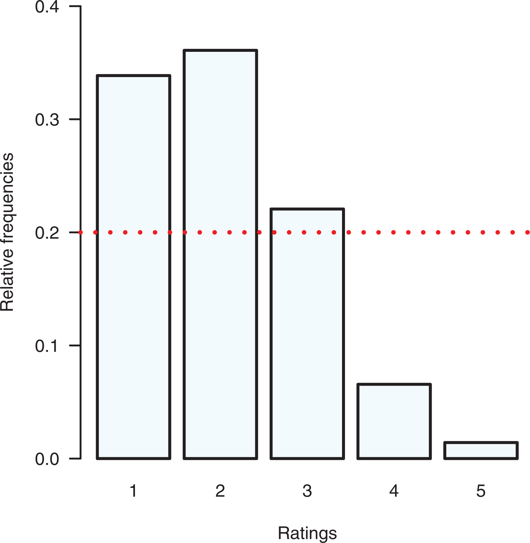
Relative frequency distribution of perceived pain—Survey of Health, Ageing and Retirement in Europe data.
Table 2 lists estimated parameters
The CUP Model Fitted to Perceived Pain Assessment—SHARE Data.
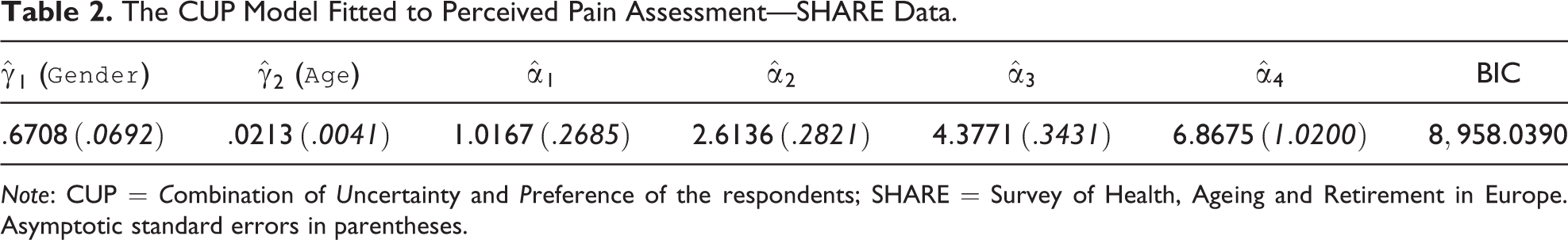
Note: CUP = Combination of Uncertainty and Preference of the respondents; SHARE = Survey of Health, Ageing and Retirement in Europe. Asymptotic standard errors in parentheses.
Given the sign convention, as expected, it is possible to observe a slightly positive effect on the female (
Thus, the probability distributions for varying
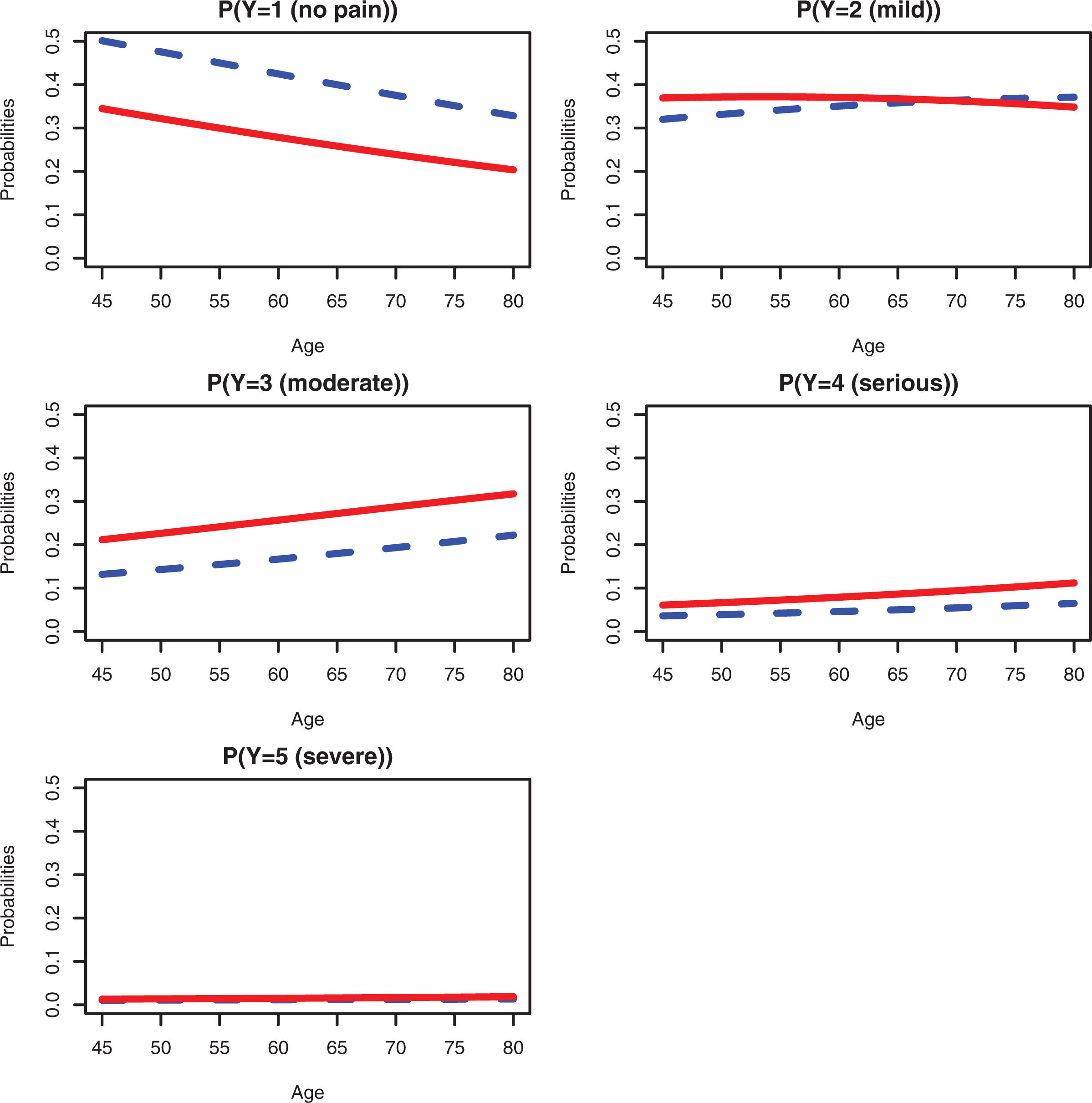
Probability of assessment for pain as function of
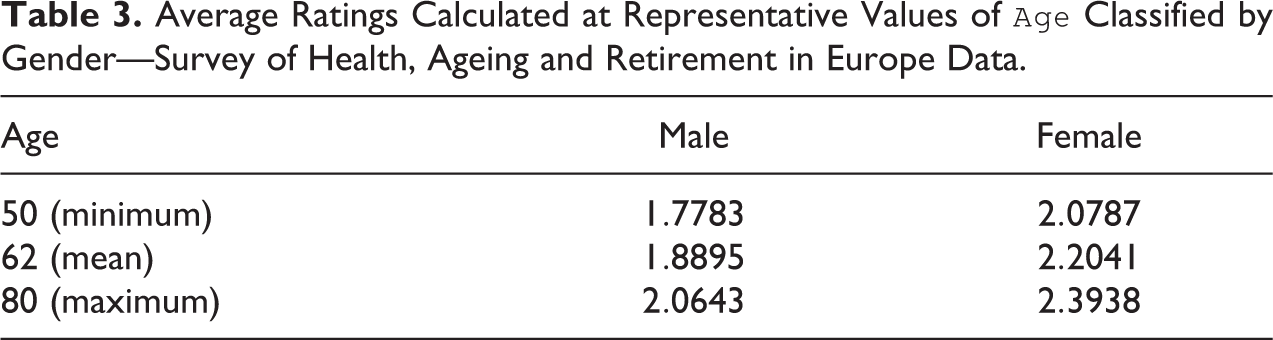
Average Ratings Calculated at Representative Values of
We then compared the observed ratings with the ones predicted by the
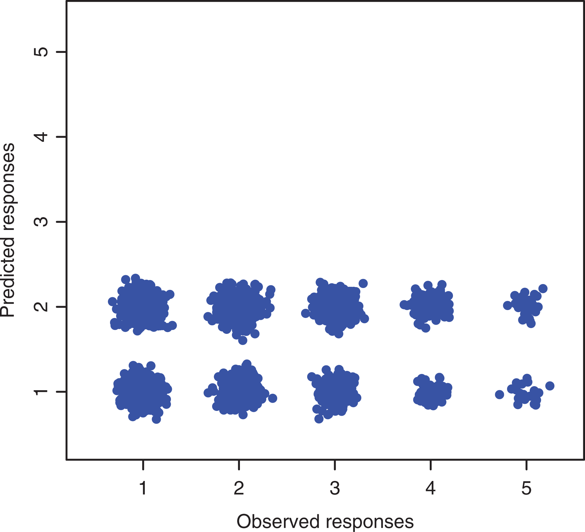
Observed and predicted responses for the Combination of Uncertainty and Preference of the respondents model—Survey of Health, Ageing and Retirement in Europe data.
ME Measures for the CUP Model—SHARE Data.
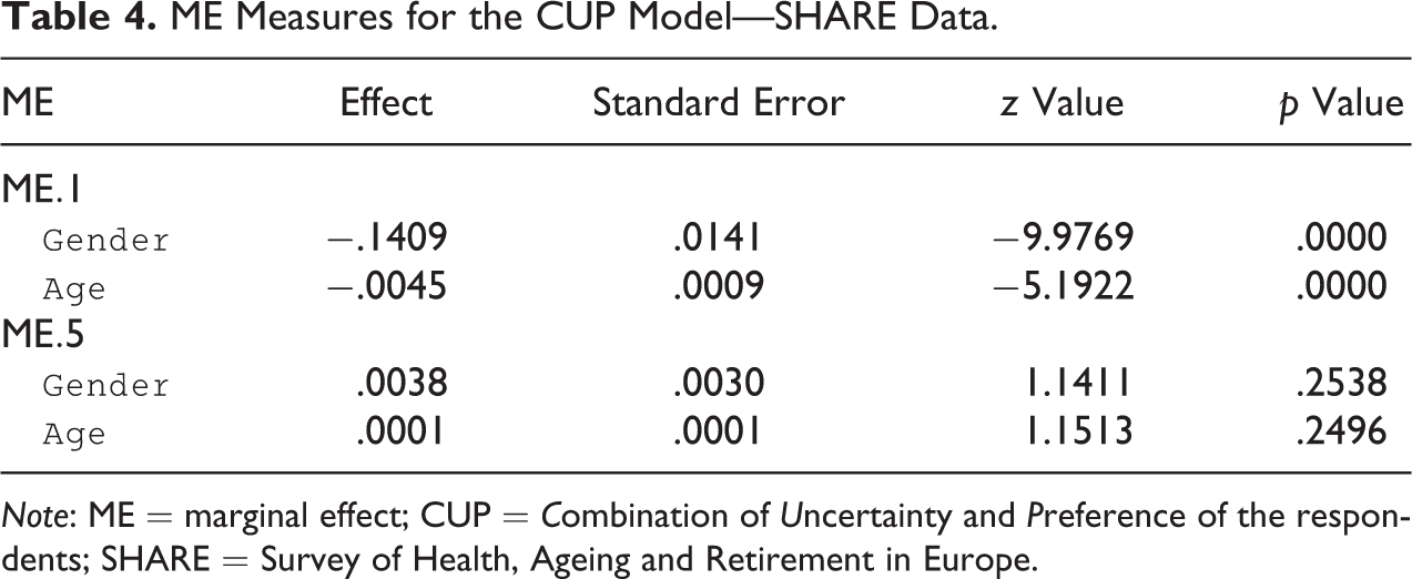
Note: ME = marginal effect; CUP = Combination of Uncertainty and Preference of the respondents; SHARE = Survey of Health, Ageing and Retirement in Europe.
In Figure 4, we report the receiver operating characteristics (ROC) curve for pain diagnostic following Tosteson et al.’s (1994) approach. The curve has been constructed using a dichotomized version of the observed ratings. It reports the false positive and true positive rates obtained as the decision threshold is varied on the different categories. Figure 4 shows that the last category (
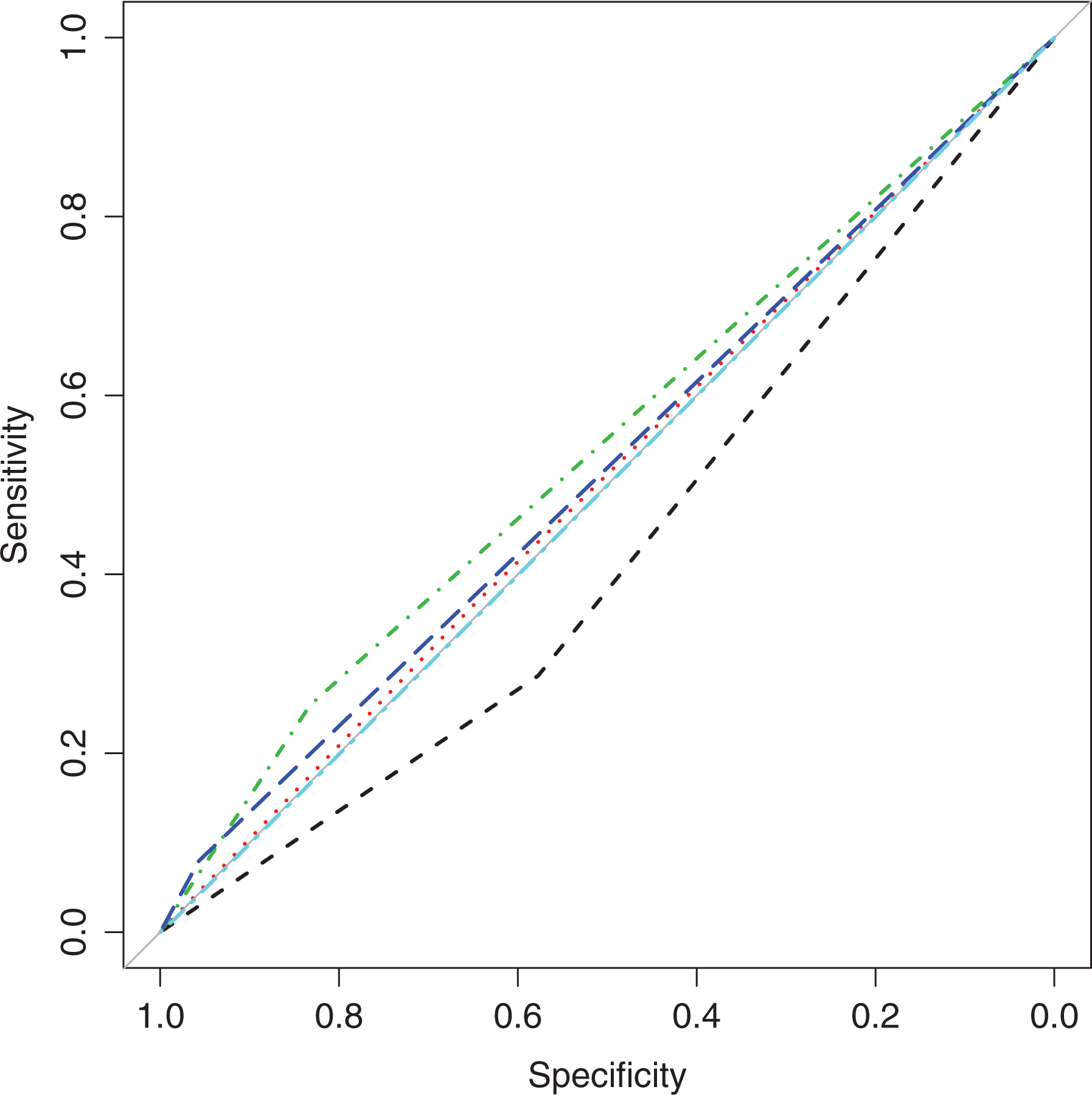
Receiver operating characteristics curves for the diagnosis of perceived pain versus categorized perceived pain—Survey of Health, Ageing and Retirement in Europe data. Note: First category is the black dashed line. Second category is the red dot line. Third category is the green dot-dashed line. The fourth category is the blue long dashed line. The fifth category is the light blue two dashed line. Areas under the curves are not significantly different with exception of the area related to the first category. Category 5 is overlapped with 45 degrees orthogonal line (no-discrimination).
The poor fitting results in terms of prediction/realization tables summarized in Figure 3, the evidence of Figure 4, and the not significant value of the ME performed on the last category point out the usefulness of merging the last two categories. Collapsing categories may be also suggested by small frequencies in the last category (
CUP Model Fitted to Perceived Pain Assessment With Collapsed Categories—SHARE Data.
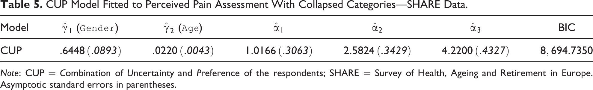
Note: CUP = Combination of Uncertainty and Preference of the respondents; SHARE = Survey of Health, Ageing and Retirement in Europe. Asymptotic standard errors in parentheses.
ME Measures for the CUP Model With Collapsed Categories—SHARE Data.
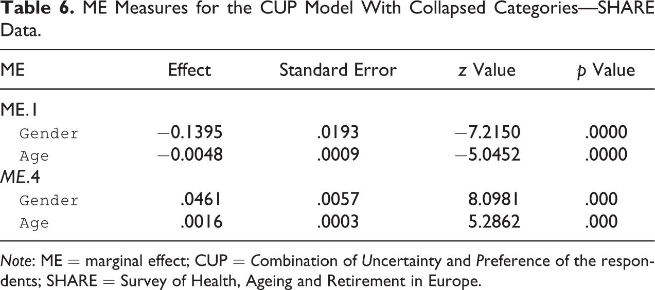
Note: ME = marginal effect; CUP = Combination of Uncertainty and Preference of the respondents; SHARE = Survey of Health, Ageing and Retirement in Europe.
The choice to collapse the last two categories enhances a discussion on the loss of efficiency (Iannario et al. 2021) because it also induces a loss of information which is reflected in larger asymptotic standard deviations (Johnson and Albert 1999; Whitehead 1993). Since the variance of the estimators is a decreasing function of k, the opportunity of merging categories should be carefully evaluated. In this case, the efficiency ratio between the before merging estimator and the after merging estimator of
In Figure 5, we present the group comparison (male and female vs.
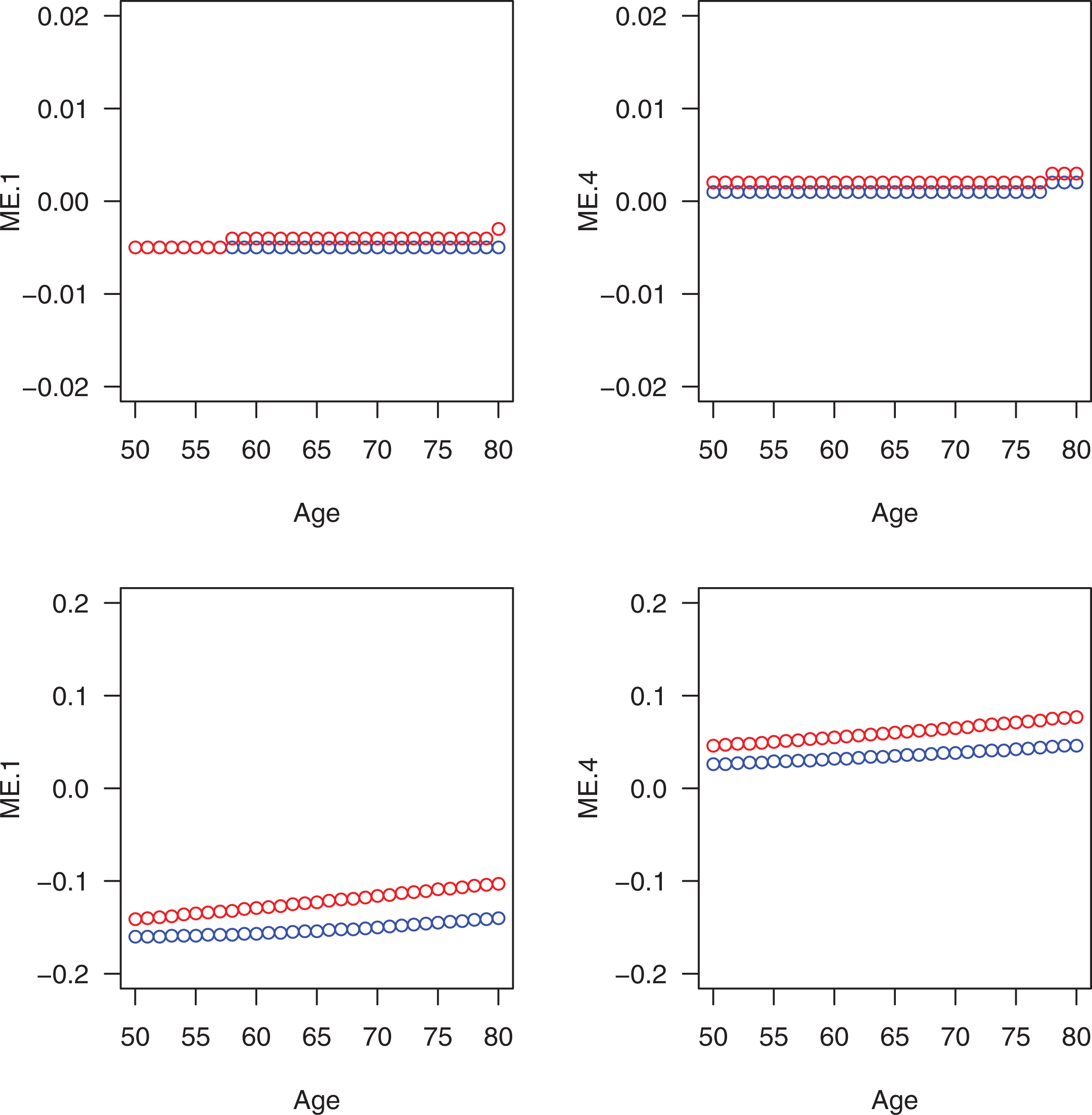
Group comparisons (male and female vs.
We proceed with the analysis of this data set with collapsed categories of pain perception evaluating the effect of the introduction of a covariate on the uncertainty component. As a covariate, we consider the handgrip (
CUP Model Fitted to Perceived Pain Assessment With Covariate on the Uncertainty Component—SHARE Data.
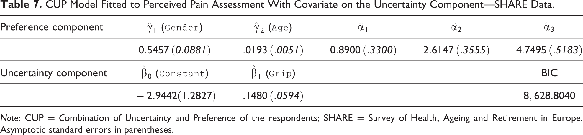
Note: CUP = Combination of Uncertainty and Preference of the respondents; SHARE = Survey of Health, Ageing and Retirement in Europe. Asymptotic standard errors in parentheses.
Before discussing the results, we would like to remind to the reader that the weight of the uncertainty component of the mixture is given by
ME Measures for the CUP Model With Collapsed Categories—SHARE Data.
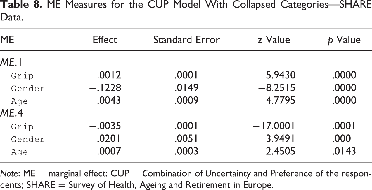
Note: ME = marginal effect; CUP = Combination of Uncertainty and Preference of the respondents; SHARE = Survey of Health, Ageing and Retirement in Europe.
European Social Survey (ESS) Data
As a further illustration, we consider a set of data from round 5 (2010) of the ESS. The sample of 38,641 respondents is available at http://ess.nsd.uib.no/ess/round5/. The ESS is a cross-national survey that has been conducted across Europe on biennial basis since 2001. Face-to-face interviews were conducted to measure the attitudes, beliefs, and behavior patterns of the examined populations. We apply a
The observable variable in Figure 6 is analyzed by means of a
Relative frequency distribution of perceived health—European Social Survey data.
CUP Model Fitted to Perceived Health—ESS Data.
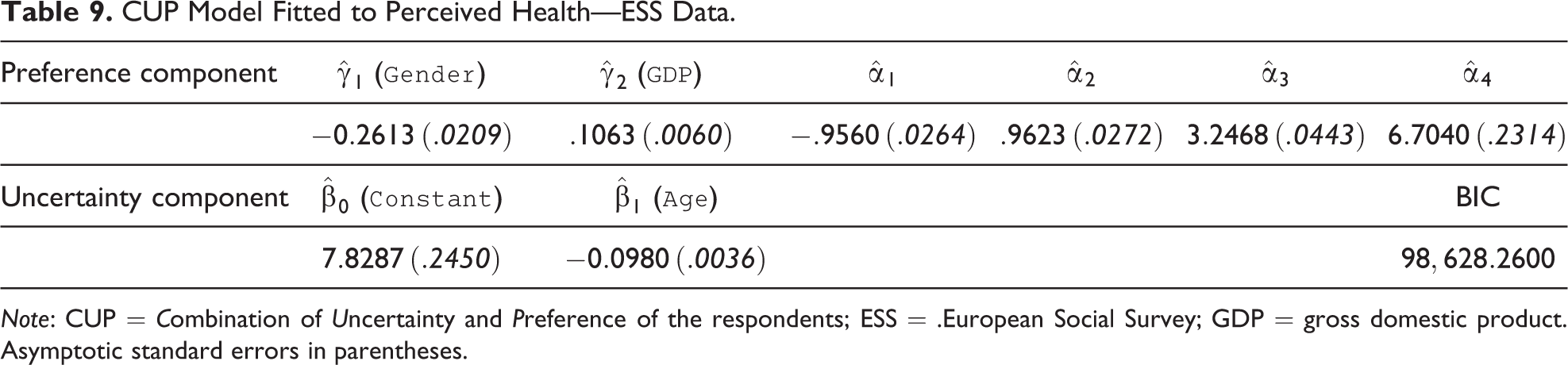
Note: CUP = Combination of Uncertainty and Preference of the respondents; ESS = .European Social Survey; GDP = gross domestic product. Asymptotic standard errors in parentheses.
In this analysis, we focus on the role of the uncertainty component. In particular, we show how neglecting the effect of possible covariates we have an adverse effect on the MEs of the covariates employed to describe the preference component of the model.
Starting with a model without covariates affecting the uncertainty component with a log-likelihood of
Results show a negative effect on the
ME for CUP Models—ESS Data.
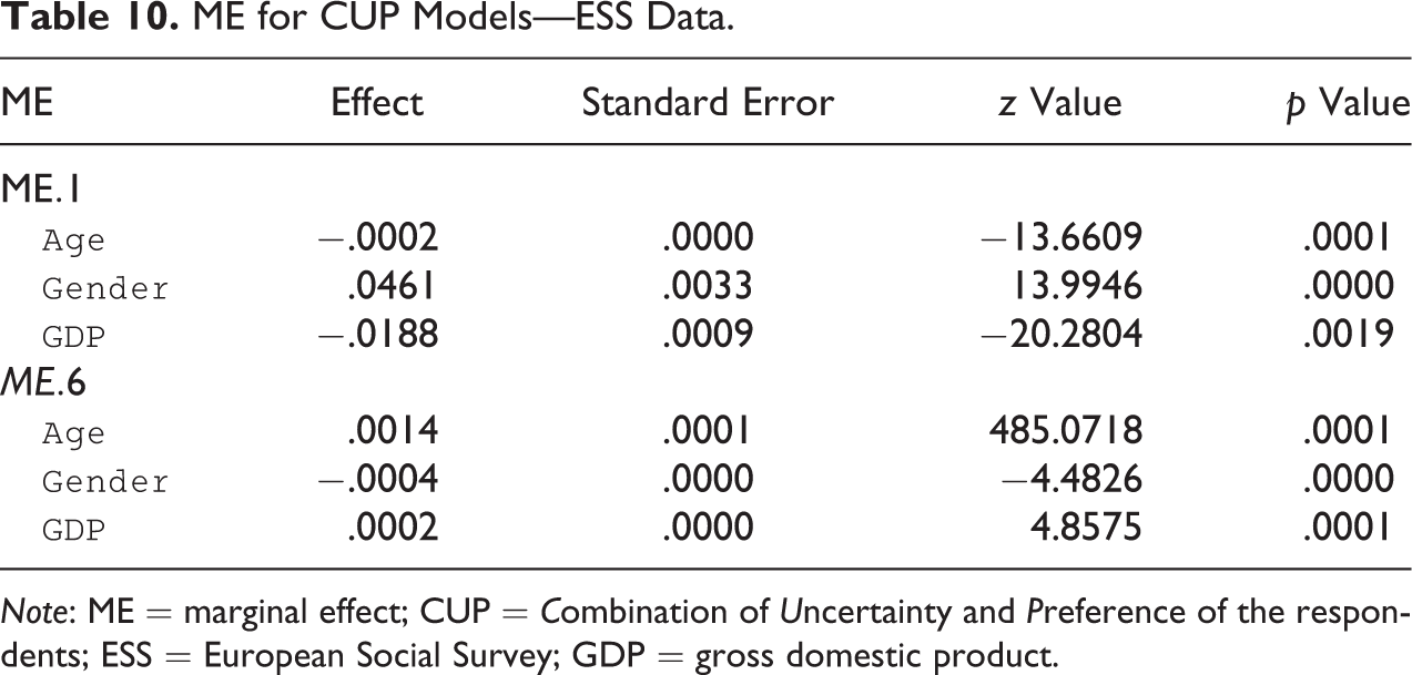
Note: ME = marginal effect; CUP = Combination of Uncertainty and Preference of the respondents; ESS = European Social Survey; GDP = gross domestic product.
The ME measures of the covariates affecting the preference component along with the asymptotic confidence intervals are displayed in Figure 7. Here, in the left panel, ME measures of the model with a fixed uncertainty component are displayed (without covariates); in the right panel, instead, there are the ME measures of the model with a covariate on the uncertainty component. The analysis underlines the loss of information obtained when a model with covariates affecting only on the preference component is examined.
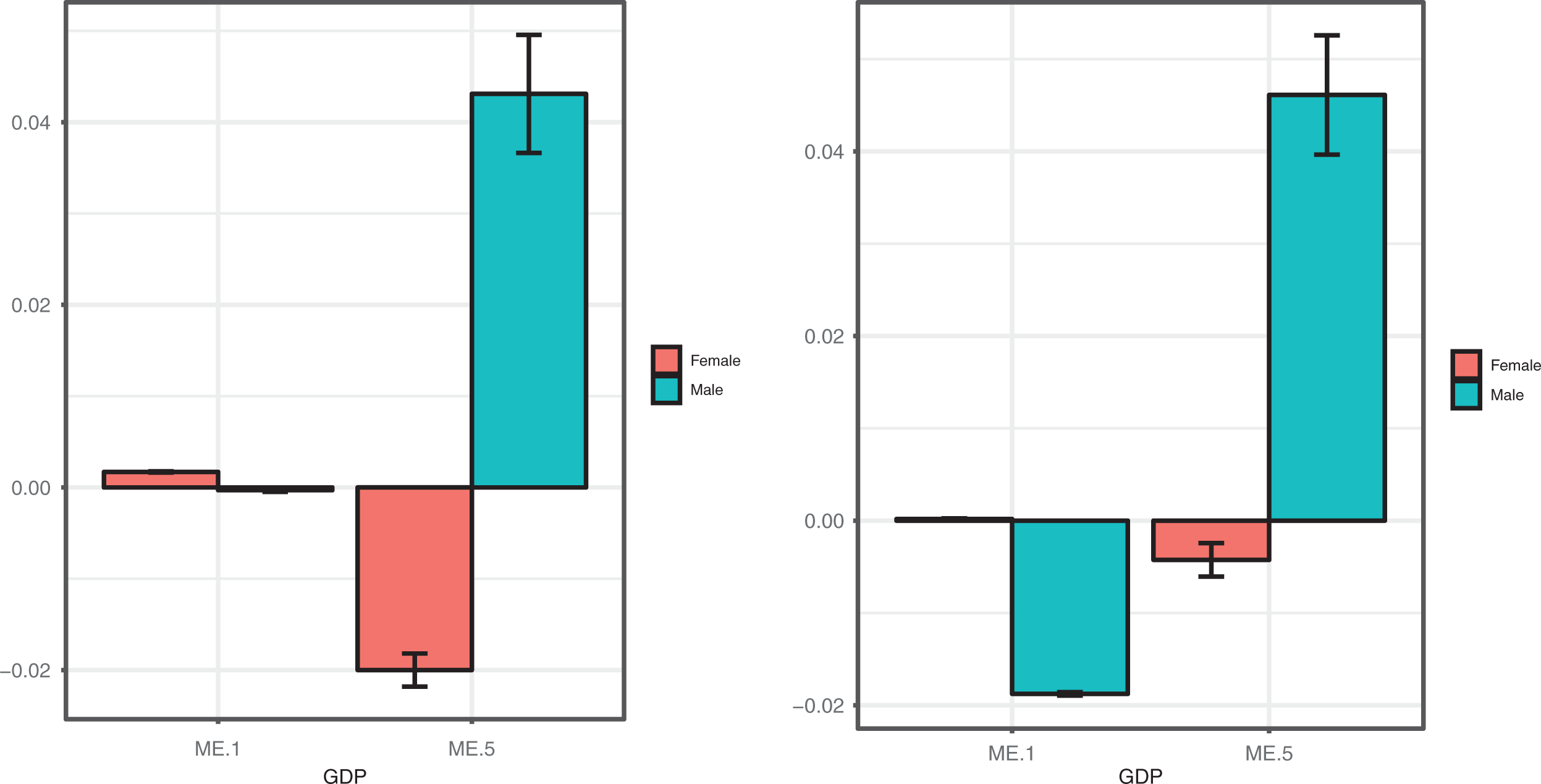
Marginal effect measures for the first category (high perceived health status) and last category (low perceived health status) by varying
Survey on Household Income and Wealth (SHIW) Data
The SHIW has been conducted by the Bank of Italy since 1965 to collect information on the economic behavior of Italian households and specifically to measure income and wealth components. The basic statistical unit is the household, defined as a group of individuals linked by ties of blood, marriage, or affection, sharing the same dwelling and pooling all or part of their incomes. Data collection is entrusted to a specialized company, and the interview stage is preceded by a series of meetings at which officials from the Bank of Italy and representatives of the company give instructions directly to the interviewers. The sample includes approximately 8,000 households and is drawn using a two-stage sample design. The questionnaire also collects information on demographics, consumption, savings, and several other topics. The number of validated observations for the empirical analysis of 2016 sample survey is 7,420 individuals. Among the several variables, the survey asks whether respondents consider their income sufficient to see the family through to the end of the month: This ordinal variable, named
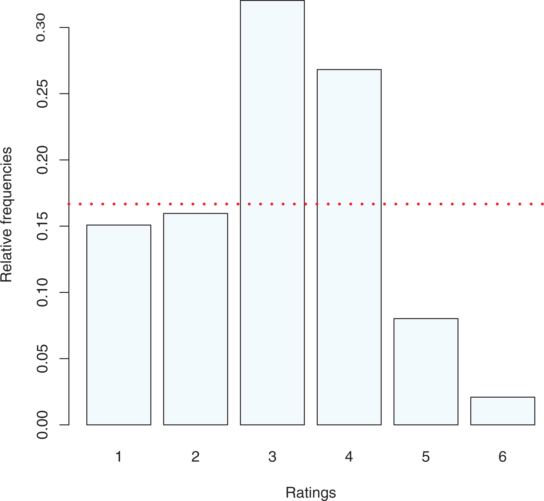
Relative frequency distribution of perceived
We analyze these data applying a
In particular, we consider the following latent model for the preference component

Results of estimation are reported in Table 11 (with a low level on uncertainty
CUP Model Fitted to Perceived Family Condition—SHIW Data.
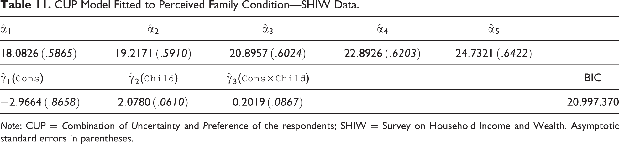
Note: CUP = Combination of Uncertainty and Preference of the respondents; SHIW = Survey on Household Income and Wealth. Asymptotic standard errors in parentheses.
ME Measures for the CUP Model—SHIW Data.
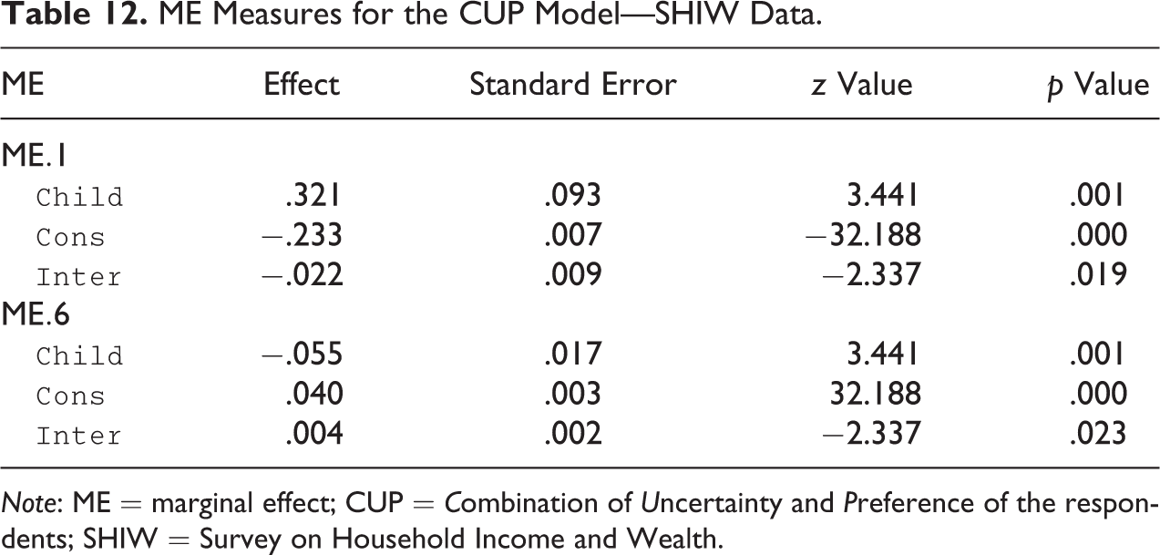
Note: ME = marginal effect; CUP = Combination of Uncertainty and Preference of the respondents; SHIW = Survey on Household Income and Wealth.
Given the sign convention, it is possible to observe a positive effect of Consumption (
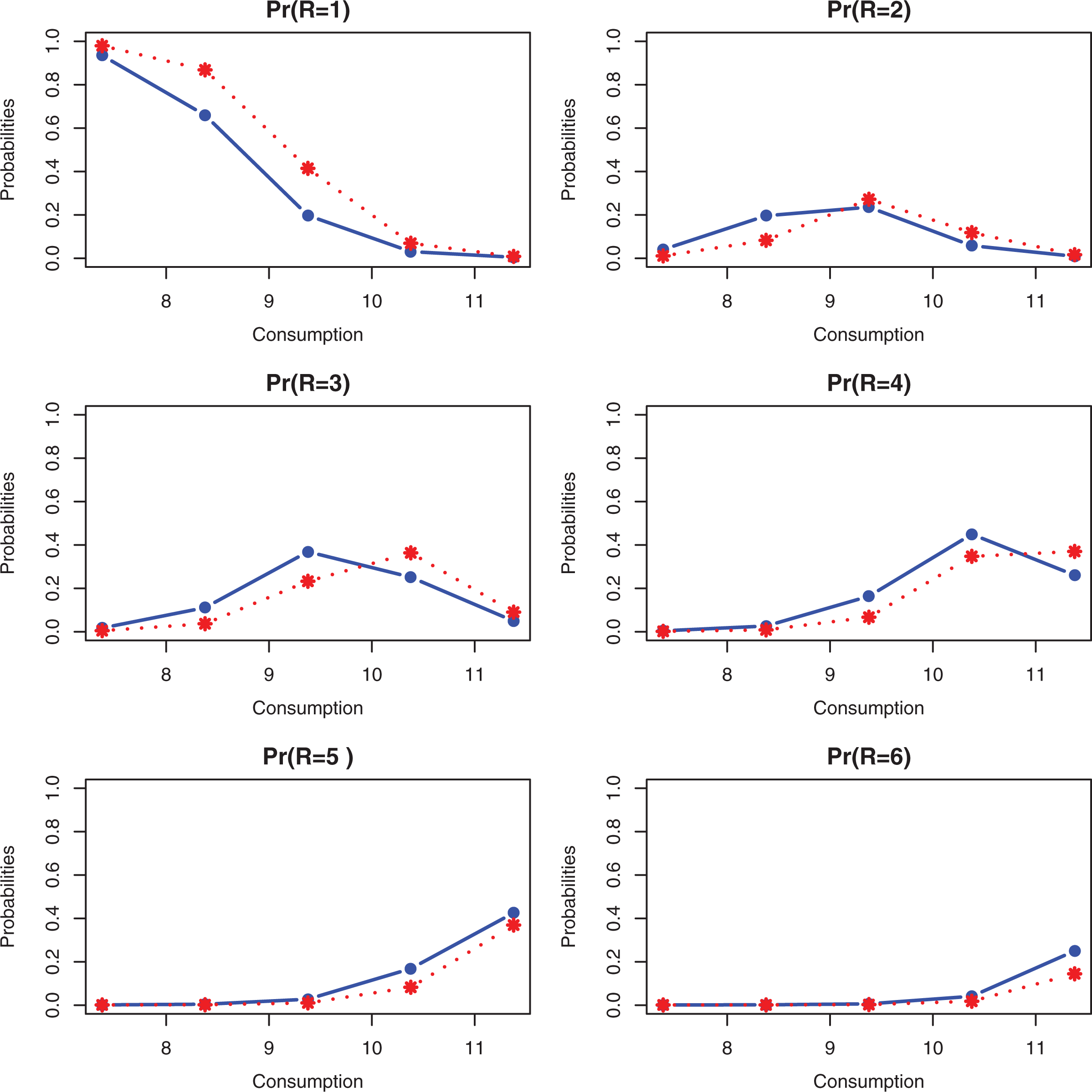
Probability of assessment for perceived family condition as function of consumption for given child (no child, blue; having child, red)—Survey on Household Income and Wealth data.
American National Election Study (ANES) Data
Studies of presidential election attract increasing attention in the field of political, economic, and other social sciences. One of the traditional research questions is how party identification relates to respondents’ voting behavior (Bartels 2000; Miller 1991) or perception of their self left–right placement, an element influencing their behavior (Lesschaeve 2017).
We consider a set of data from the 1996 ANES project developed by the Institute for Social Research of the University of Michigan (https://www.icpsr.umich.edu/icpsrweb/ICPSR/series/00003). It regard voting preferences on Clinton political position. It is also available in the R package
The examined data frame consists of 944 observations. We analyze these data applying a
The ordinal response variable is self left–right placement expressed on a seven-point Likert-type scale from 1 = extremely liberal to 7 = extremely conservative (Figure 10 shows the relative frequency distribution). Parameter estimation of the

Relative frequency distribution of self left–right placement—American National Election Study data.
CUP Models Fitted to Self Left–Right Placement—ANES Data.
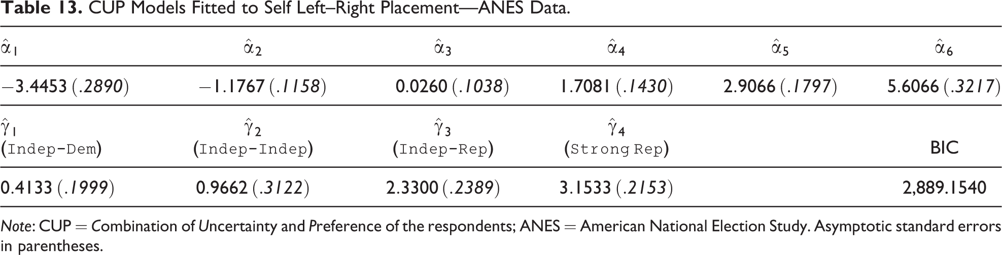
Note: CUP = Combination of Uncertainty and Preference of the respondents; ANES = American National Election Study. Asymptotic standard errors in parentheses.
Figure 11 reports the probability of the extreme categories of the ordinal variables given

Individual marginal effects at representative values of covariates (
ME for the CUP Model—ANES Data.
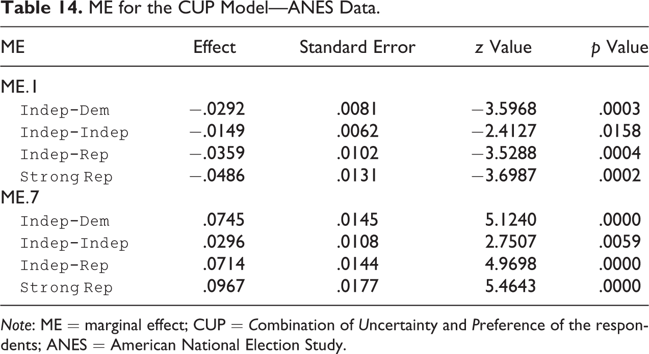
Note: ME = marginal effect; CUP = Combination of Uncertainty and Preference of the respondents; ANES = American National Election Study.
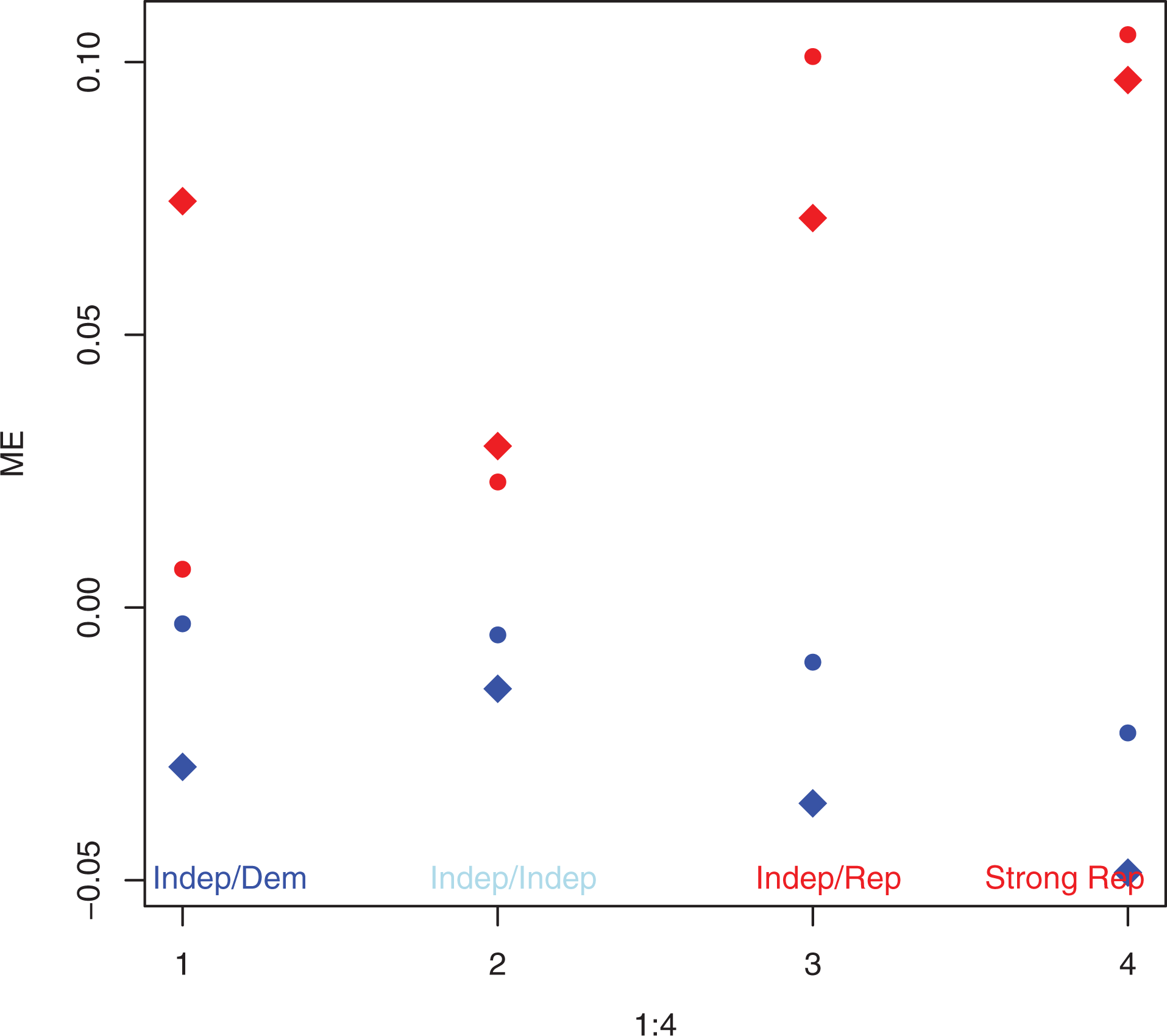
Marginal effect (ME) for the first category “extremely conservative’ (blue) and last category “extremely liberal” (red) by varying party identification—American National Election Study data. Note: Dots represent ME measures computed on the standard proportional odds model without taking into account the uncertainty component. Diamonds represent ME measures computed on the Combination of Uncertainty and Preference of the respondents model. The size of diamond is scaled on the uncertainty measure.
Concluding Remarks
The aim of this article has been to introduce effect measures that can be easier to interpret than model parameters for ordinal response models with uncertainty component. The measures discussed in this article extend to the examined context some previous results and implement new topics in case of interaction among covariates.
The article highlights by means of the analysis of ME measures that when the uncertainty component is neglected, the strength of the covariates tends to be underestimated. Readers who find challenging to understand cumulative link models with corresponding summary measures such as odds ratios undoubtedly find such generalized models even more demanding. When effects are monotone, simple summaries such as changes over the range in estimated ordinal extreme-category probabilities could be useful to help readers understand the substantive importance of the effects, and they can be presented with simple graphical devices. Extreme ME measures may also help to understand possible response styles and motivate collapsing of extreme categories (as the example on SHARE data shows).
The reported examples illustrate different use of ME measures changing the explanatory covariates and the main topic by stressing the role of these measures and their possible implementation in different contexts. A natural extension of this work may be to present effect measures for other models such as generalized additive models for ordinal responses with uncertainty or nominal response models.
Furthermore, by considering a recent development that replaces the uniform in a
An alternative approach may be the analysis of ME measures for ordinal data models that take into account the “don’t know” option as in Iannario et al. (2020) or ME interpretation in case where the data generating process results into too many zeroes as for zero-inflated ordinal data models (see Harris and Zhao 2007). Finally, although this article is developed in a frequentist framework, it could be of interest to study the corresponding counterpart measures in a Bayesian setting. Naturally, this next study should take into account Bayesian model estimation and selection and the corresponding computational issues.
Supplemental Materials
Supplemental Material, sj-eps-1-smr-10.1177_0049124120986179 - How to Interpret the Effect of Covariates on the Extreme Categories in Ordinal Data Models
Supplemental Material, sj-eps-1-smr-10.1177_0049124120986179 for How to Interpret the Effect of Covariates on the Extreme Categories in Ordinal Data Models by Maria Iannario and Claudia Tarantola in Sociological Methods & Research
Supplemental Materials
Supplemental Material, sj-eps-2-smr-10.1177_0049124120986179 - How to Interpret the Effect of Covariates on the Extreme Categories in Ordinal Data Models
Supplemental Material, sj-eps-2-smr-10.1177_0049124120986179 for How to Interpret the Effect of Covariates on the Extreme Categories in Ordinal Data Models by Maria Iannario and Claudia Tarantola in Sociological Methods & Research
Supplemental Materials
Supplemental Material, sj-eps-3-smr-10.1177_0049124120986179 - How to Interpret the Effect of Covariates on the Extreme Categories in Ordinal Data Models
Supplemental Material, sj-eps-3-smr-10.1177_0049124120986179 for How to Interpret the Effect of Covariates on the Extreme Categories in Ordinal Data Models by Maria Iannario and Claudia Tarantola in Sociological Methods & Research
Supplemental Materials
Supplemental Material, sj-tex-1-smr-10.1177_0049124120986179 - How to Interpret the Effect of Covariates on the Extreme Categories in Ordinal Data Models
Supplemental Material, sj-tex-1-smr-10.1177_0049124120986179 for How to Interpret the Effect of Covariates on the Extreme Categories in Ordinal Data Models by Maria Iannario and Claudia Tarantola in Sociological Methods & Research
Footnotes
Declaration of Conflicting Interests
The author(s) declared no potential conflicts of interest with respect to the research, authorship, and/or publication of this article.
Funding
The author(s) received no financial support for the research, authorship, and/or publication of this article.
Supplemental Materials
Supplemental material for this article is available online.
References
Supplementary Material
Please find the following supplemental material available below.
For Open Access articles published under a Creative Commons License, all supplemental material carries the same license as the article it is associated with.
For non-Open Access articles published, all supplemental material carries a non-exclusive license, and permission requests for re-use of supplemental material or any part of supplemental material shall be sent directly to the copyright owner as specified in the copyright notice associated with the article.