
Abstract
Hierarchical linear modeling (HLM) is often used to estimate the effects of socioeconomic status (SES) on academic achievement at different levels of an educational system. However, if a prior academic achievement measure is missing in a HLM model, biased estimates may occur on the effects of student SES and school SES. Phantom effects describe the phenomenon in which the effects of student SES and school SES disappear once prior academic achievement is added to the model. In the present analysis, partial simulation (i.e., simulated data are used together with real-world data) was employed to examine the phantom effects of student SES and school SES on science achievement, using the national sample of the United States from the 2015 Programme for International Student Assessment. The results showed that the phantom effects of student SES and school SES are rather real. The stronger the correlation between prior science achievement and (present) science achievement, the greater the chance that the phantom effects occur.
Keywords
Socioeconomic status (SES) affects students’ academic achievement at different levels of an educational system such as students and schools (Organisation for Economic Co-operation and Development [OECD], 2016). Student SES is often measured through parents’ education, occupation, and income. School SES, also referred to as school socioeconomic composition, is often measured through the aggregation of SES among students within a school. School SES is, perhaps, the most popular school contextual variable, demonstrating large and persistent effects on students’ academic achievement (e.g., Caldas and Bankston 1997; Perry and McConney 2010; White 1982).
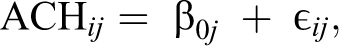
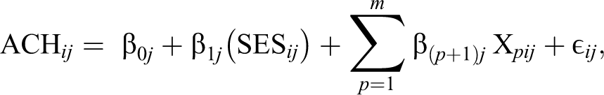
In empirical investigations of school SES in relation to students’ academic achievement, hierarchical linear modeling (HLM) is the typical statistical technique to address the issue of data hierarchy with students nested within schools. Such a HLM model is often referred to as the compositional model (see Raudenbush and Bryk 2002). With student SES at level 1 (i.e., the student level), the model is

where
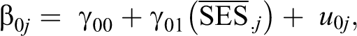
At level 2 (i.e., the school level), with
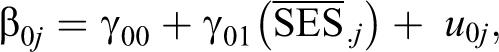
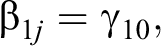
where

We call this HLM model the simplified model in that there can be student-level variables and school-level variables to function as control variables to adjust the effects of student SES and school SES at the corresponding level.
Although the use of HLM is appropriate to investigate the effects of student SES and school SES, what student-level variables and school-level variables need to be in the model as controls is an issue open to debate. There is the concern that the omission of some variables may create biases on the effects of student SES and, in particular, school SES. This matter is likely to become serious if the model omits a variable that is highly related to ACH (see Marks 2015; Pokropek 2015; Televantou et al. 2015). Prior academic achievement is one of the most relevant variables to ACH, the absence of which can alter the effects of both student SES and school SES on ACH (Marks 2015; Perry 2018).
These researchers explained how the phenomenon occurs. In the absence of students’ prior academic achievement, there are statistically significant effects of school SES on academic achievement (at the school level), but in the presence of students’ prior academic achievement, the statistically significant effects of school SES tend to decrease or disappear. They referred to this phenomenon as fake compositional effects, statistical artifacts, or phantom effects. In the present analysis, we adopted the term phantom effects. Conceptually, phantom effects are defined as the effects of A on a certain outcome in the absence of B, which tend to disappear in the presence of B. Obviously, in the context of HLM, phantom effects can occur at any level of the model.
As an example, Marks (2015) investigated whether students’ prior academic achievement influences the estimation of the effects of school SES on students’ present academic achievement within the HLM framework. The data came from the Victorian sector of the (Australian) National Assessment Program—Literacy and Numeracy (NAPLAN). The program aims to test the academic development of students in Year 3, 5, and 7 (corresponding calendar years are 2008, 2010, and 2012). The tests are all equated. Student SES contains two measures (parents’ occupation and parents’ education). School SES is calculated as the mean SES of students within each school. When examining students’ academic achievement in Year 7, Marks (2015) treated students’ academic achievement in Year 3 and Year 5 as prior academic achievement. Using a model similar to the HLM model that we discussed earlier, Marks (2015) showed that, after controlling for students’ prior academic achievement, the statistically significant effects of school SES on students’ academic achievement in Year 7 disappeared in both cases of SES measures (i.e., both parents’ occupation and parents’ education).
Phantom effects are actually not an entirely new phenomenon in the educational realm. Take the example of SES and racial-ethnic differences in academic achievement. In the absence of SES, racial-ethnic differences are often statistically significant in academic achievement among students. However, in the presence of SES, such statistically significant effects often decrease or disappear, which makes racial-ethnic differences phantom effects (i.e., SES is the root of the problem).
Scholars have long argued that the relationship between SES and academic achievement among students can be mediated by students’ prior academic achievement (see Marks 2017). Nonetheless, the issue has never been investigated from the perspective of phantom effects. At the same time, researchers have just begun to understand phantom effects concerning school contextual composition. Very few studies have investigated the effects of school SES on students’ academic achievement in the presence of prior students’ academic achievement. We aim to examine the extent to which the effects of student SES and school SES on students’ academic achievement are phantom effects. Data for the present analysis come from the 2015 Programme for International Student Assessment (PISA) with an emphasis on science education. With students nested within schools, PISA data are appropriate for research on individual differences and school effects. To examine the potential phantom effects of student SES and school SES, our strategy is to generate a prior measure of science achievement with various degrees of correlation with the PISA 2015 measure of science achievement. With the HLM models fitted with and without these prior science achievement measures, the behaviors of student SES and school SES can be examined in terms of their effects on science achievement. We attempt to address the following research questions. In the absence of prior science achievement measures, how strong are the effects of student SES and school socioeconomic composition (i.e., school SES) on science achievement of students with and without control for student characteristics and school characteristics? In the presence of prior science achievement measures, how strong are the effects of student SES and school socioeconomic composition (i.e., school SES) on science achievement of students with and without control for student characteristics and school characteristics?
The combination of empirical answers to these questions provides evidence to address the issue concerning the extent to which the effects of student SES and school SES on students’ science achievement are phantom effects.
Method
Data
In the present analysis, we employed the national probability sample of the United States (U.S.) from the 2015 PISA. PISA measures 15-year-old school students’ scholastic performance in three academic fields (reading, mathematics, and science). Since 2000, PISA has been carried out every 3 years, with a rotating emphasis on reading, mathematics, and science. The latest cycle of 2015 focused on science (OECD 2016). Apart from academic achievement tests, PISA contains information that reasonably describes students, teachers, and schools (measured through student and school questionnaires).
The PISA sampling design is a probabilistic, stratified, and randomized cluster design. Schools are randomly selected first with probability proportional to some school characteristics. Students within each sampled school are then randomly selected with equal probability. Sampling weights apply to both schools and students (OECD 2016). In terms of the U.S. national sample, the population of schools that have the 10th grade (corresponding to 15-year-old students) is stratified by geographic region (Northeast, Central, West, and Southeast) and school type (public and private). Within each stratum, schools are further stratified by state, school grade, school location (city, suburb, town, and rural), school gender composition (percentage of male students above 95, percentage of female students above 95, and others), and school racial-ethnic composition (percentage of Black, Hispanic, Asian, Native Hawaiian or Pacific Islander, and American Indian or Alaska Native students below or above 15). Within each sampled school, 42 students who are 15 years old are randomly selected. Finally, the U.S. national sample contains 5,712 students from 177 schools. The use of nationally representative data increases the credibility and generalizability of the present analysis.
Variables
The dependent variable was students’ science achievement in the present analysis. PISA uses the term of science literacy defined as “the ability to understand the characteristics of science and the significance of science in our modern world, to apply scientific knowledge, identify issues, describe scientific phenomena, draw conclusions based on evidence, and the willingness to reflect on and engage with scientific ideas and subjects” (OECD 2009:22). Students’ scores are estimated based on plausible values because each student completes a subset of the test items (referred to as matrix sampling). The idea of plausible values is that, for each student, a number of random values are drawn from certain established posterior distributions (see OECD 2009:96). PISA 2015 contains 10 plausible values for each student to represent his or her science achievement, and each plausible value contains information about the estimation on the ability of the student and the uncertainty of the estimation (OECD 2016). Therefore, plausible values are not real test scores, but there is a standard procedure to integrate plausible values when conducting analysis to produce a score in the traditional sense for each student (OECD 2009). The PISA 2015 science achievement has a scale with a mean of 500 and a standard deviation (SD) of 100 (OECD 2016).
There were independent variables at both student and school levels. At the student level, we selected variables that are exogenous in nature to function as controls over individual differences (see Ma, Ma, and Bradley 2008). Student characteristics included gender, age, SES, immigration status, and home language. Other desirable exogenous variables including race–ethnicity were not available in PISA 2015.
At the school level, we included major contextual and climate variables (see Ma et al. 2008). Contextual variables included school (enrollment) size, school location, school ownership, and proportion of science teachers fully certified. The key contextual variable of school socioeconomic composition or school SES was aggregated from SES of students within each school. Four variables are essential to describe school climate including disciplinary climate, academic pressure, principal leadership, and parental involvement (not available in PISA 2015). Disciplinary climate and academic pressure came from information obtained at the student level and were aggregated within a school to produce school-level measures. Principle leadership came from the school questionnaire, measuring mainly principals’ instructional leadership. PISA 2015 contains items measuring directly disciplinary climate and principal leadership but contains no items measuring directly academic pressure. A proxy variable, teacher support (in a science class), was used to represent a critical aspect of academic pressure. Each of these school climate variables is made from a scale of several items and is often referred to as a composite variable (OECD 2016). Online Appendix (which can be found at http://smr.sagepub.com/supplemental/) informs how each of these variables is constructed.
Models
As a preparation for the examination of phantom effects of student SES and school SES on science achievement, a null model was run with only the dependent variable (i.e., without any independent variables at any level). The null model provided an analytical background for the present analysis, estimating essentially the intraclass correlation (ICC), which represents the proportion of variance in science achievement that was attributable to the school level. The null model was expressed as
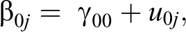
where
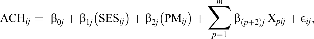
We adopted a general analytical framework with a four-step approach to examine the phantom effects of student SES and school SES on schooling outcomes (see Ma and Zhou 2018). The base model (in the first step) was essentially the same as the (contextual) HLM that we discussed at the beginning. The purpose was to measure the absolute effects of student SES and school SES without any adjustment of other variables at either level. In the second step, we introduced prior science achievement (simulated to have various strength of correlation with the PISA science achievement measure). The purpose was to examine whether the absolute effects would change once prior science achievement was introduced at the student level. This model was expressed as


where all parameters that we discussed earlier hold the same meanings. Meanwhile,
Ma and Zhou (2018) referred to the two models above as the set of absolute models for phantom effects. The term, absolute, indicates that the influence of prior science achievement is examined in the absence of other variables at the student and school levels. In the next two steps, variables at the student and school levels were introduced to the absolute models. Ma and Zhou (2018) referred to these models as the set of relative models for phantom effects. The term, relative, indicates that the influence of prior science achievement is examined in the presence of other variables at the student and school levels.
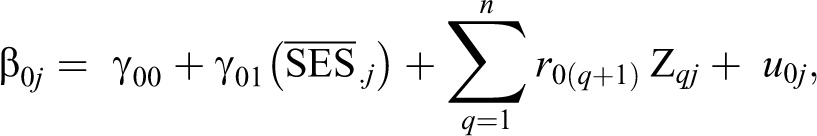
Specifically, in the third step, we introduced variables to the base model at the student and school levels. These variables provided adjustments at the student and school levels to purify the effects of student SES and school SES on science achievement. The purpose was to measure the relative effects of student SES and school SES. This model was expressed as


where
In the final (fourth) step, we introduced prior science achievement (simulated to have various strength of correlation with the PISA science achievement measure). The purpose was to examine whether the relative effects would change once prior science achievement was introduced at the student level. This model was expressed as

where all parameters hold the same meanings as we discussed earlier.
Simulation
Because PISA does not have prior academic achievement measures, we generated prior measures of science achievement in the present analysis. Simulated data would then work with actual data to address a statistical issue, thus named partial simulation. The procedure was to generate a random variable with a defined correlation to the dependent variable (i.e., the PISA science achievement measure). The conditions manipulated were the correlation between the dependent variable and the created variables. Nine correlations were considered (.15, .25, .35, .45, .55, .65, .75, .85, and .95), and the generated variables were used as prior measures of science achievement. For each prior measure, a set of HLM analyses were performed with models that we discussed in the previous section. As a result, nine sets of HLM analyses were performed.
Analysis
What made the partial simulation procedure far more complicated in the present analysis was the fact that there were ten plausible values in the 2015 PISA data. So, we needed to work with plausible values when conducting our partial simulation study. According to OECD (2009:104), there are four steps to integrate plausible values. Applied to the present analysis, the first step specified each plausible value as a dependent variable in a certain regression model. For a certain regression coefficient of interest, a total of 81 regression analyses were performed with the final weight and the 80 replicate weights. Overall, with 10 plausible values, 810 estimates on the regression coefficient were generated to produce 10 sampling variances (one for each plausible value). The second step calculated the average of the 10 estimates on the regression coefficient (based on the final weight) and the average of the 10 sampling variances to produce the final estimates for the regression coefficient and the sampling error. The third step calculated the imputation variance. The final step calculated the standard error. This procedure was applied to each of the four HLM models that we discussed earlier.
To work with missing data in PISA 2015, OECD (2009) suggests a single imputation. Applied to the present analysis, for a continuous variable, a missing value was replaced by the weighted school mean. If the weighted school mean could not be calculated, the missing value was replaced by the weighted country mean. The final weight was applied for each weighted mean. For a dichotomous variable, a missing value is replaced by zero. All the following HLM analyses were based on these treatments.
Results
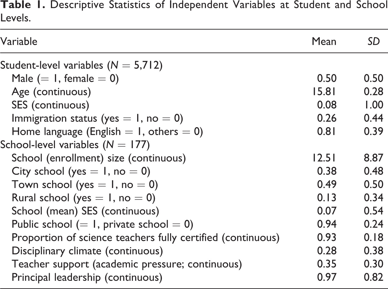
Table 1 presents the descriptive statistics of variables in the present analysis. We used the null HLM models to provide some background for all the subsequent HLM analyses. On the PISA academic achievement scale with a mean of 500 and a SD of 100, the national average of science achievement among students in the U.S. was 494 points. The variance in science achievement in the U.S. was 7,727.50 at the student level and 1,876.65 at the school level (this amount was statistically significant). The ICC was .20, indicating that 20 percent of the total variance in science achievement was attributable to schools.
Descriptive Statistics of Independent Variables at Student and School Levels.
Absolute Phantom Effects
Table 2 presents the analytical results on the effects of student SES and school SES in the absence of student and school background variables before and after the addition of prior science achievement measures (i.e., the absolute effects models). Within this table, the panel labeled as “no prior” indicates the base model. Both student SES and school SES had positive and strong effects on student science achievement. For one unit increase in student SES, student science achievement would increase by 22.84 points; and for one unit increase in school SES, student science achievement would increase by 35.78 points. Because the PISA science achievement scale has a SD = 100, an effect size measure as the proportion of one SD can be easily calculated. As a result, the absolute effects of student SES was .23 SD in effect size on student science achievement, and the absolute effects of school SES was .36 SD in effect size on student science achievement.
Changes in Absolute Effects of Student SES and School SES on Science Achievement With and Without Prior Measures of Science Achievement.
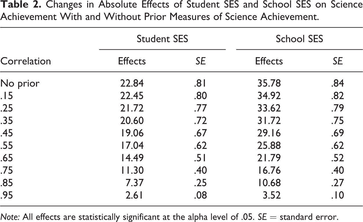
Note: All effects are statistically significant at the alpha level of .05. SE = standard error.
The rest of the panels in Table 2 all have the addition of prior science achievement in various correlations with (present) science achievement (i.e., the PISA science achievement). With the correlation increasing from .15 to .95, the absolute effects of student SES on student science achievement decreased from 22.45 to 2.61 (with effect size decreasing from .22 SD to .03 SD), and the absolute effects of school SES on student science achievement decreased from 35.78 to 3.52 (with effect size decreasing from .36 SD to .04 SD).
These results clearly showed that the presence of a prior science achievement measure dramatically decreased the absolute effects of both student SES and school SES on student science achievement. The stronger the correlation between prior science achievement and (present) science achievement, the greater the decrease in the absolute effects of both student SES and school SES.
If 25 percent of a SD can be considered as the cut-off point for practical importance (see Cohen 1988), then the absolute phantom effects of school SES can occur when prior science achievement has a correlation of .65 (or even .55) with (present) science achievement. Meanwhile, even though the absolute effects of student SES are all below the cut-off point, when prior science achievement has a correlation of .65 with (present) science achievement, the first disproportional drop in the absolute effects of student SES occurs.
Relative Phantom Effects
Table 3 presents the analytical results on the effects of student SES and school SES in the presence of student and school background variables before and after the addition of prior science achievement measures (i.e., the relative effects models). To focus on the effects of student SES and school SES on student science achievement, this table has omitted statistical information pertaining to the effects of other student and school characteristics. Within this table, the panel labeled as “no prior” indicates the full model (with student and school background variables). Even after control over student and school characteristics, both student SES and school SES had positive and strong effects on student science achievement. With statistical control over student and school characteristics, for one unit increase in student SES, student science achievement would increase by 20.95 points (i.e., an effect size of .21 SD); and for one unit increase in school SES, student science achievement would increase by 27.16 points (i.e., an effect size of .27 SD).
Changes in Relative Effects of Student SES and School SES on Science Achievement With and Without Prior Measures of Science Achievement.
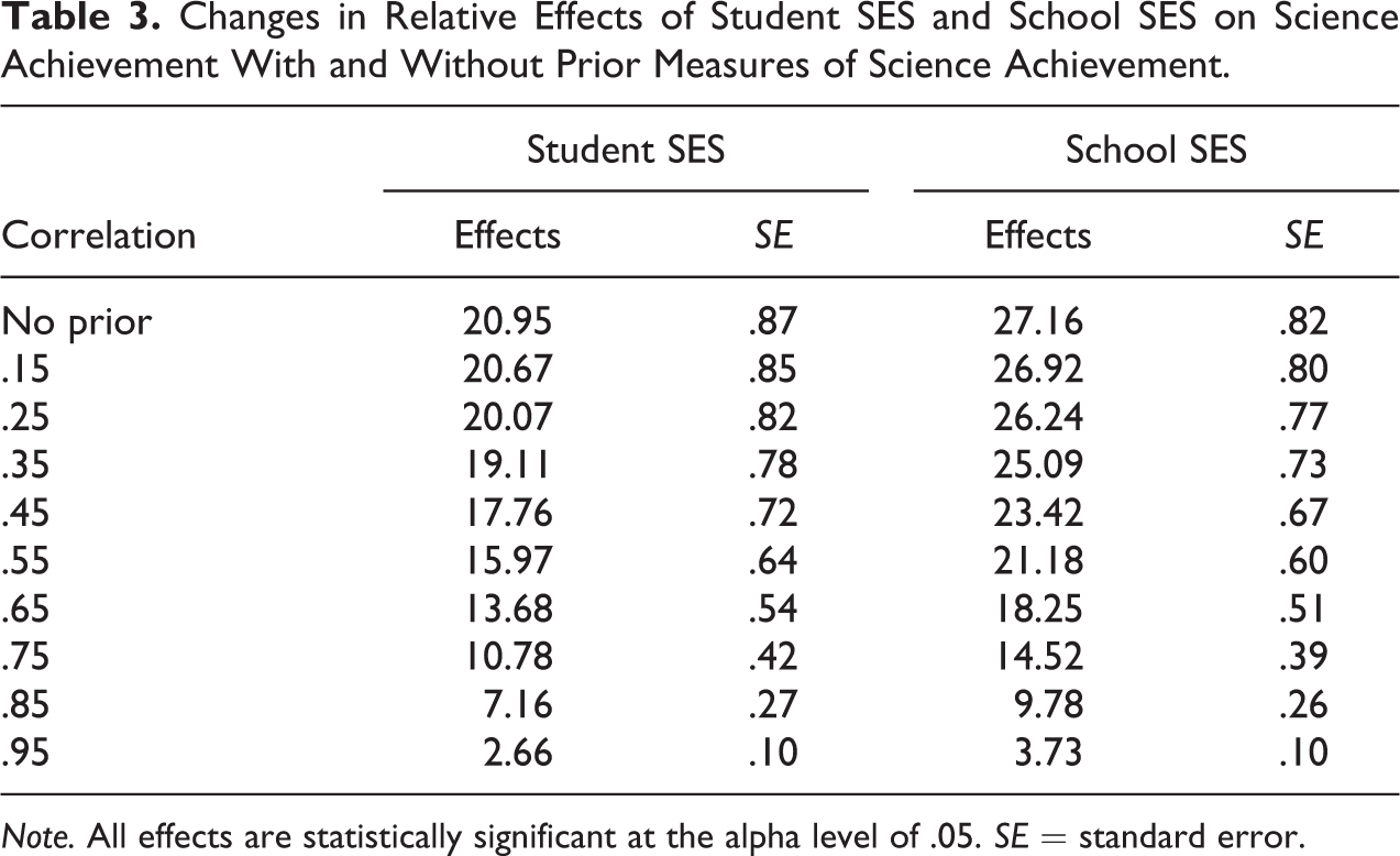
Note. All effects are statistically significant at the alpha level of .05. SE = standard error.
The rest of the panels in Table 3 all have the addition of prior science achievement in various correlations with (present) science achievement (i.e., the PISA science achievement). With the correlation increasing from .15 to .95, the relative effects of student SES on student science achievement decreased from 20.67 to 2.66 (with effect size decreasing from .21 SD to .03 SD), and the relative effects of school SES on student science achievement decreased from 27.16 to 3.73 (with effect size decreasing from .27 SD to .04 SD).
These results clearly showed that, even after statistical control over important student and school characteristics (at the student and school levels respectively), the presence of a prior science achievement measure still dramatically decreased the relative effects of both student SES and school SES on student science achievement. The stronger the correlation between prior science achievement and (present) science achievement, the greater the decrease in the relative effects of both student SES and school SES.
Again, using 25 percent of a SD as the standard for practical importance, in the presence of student and school characteristics, the relative phantom effects of school SES can occur when prior science achievement has a correlation of .45 (or even .35) with (present) science achievement. Meanwhile, even though the relative effects of student SES are all below the standard, when prior science achievement has a correlation of .45 with (present) science achievement, the first disproportional drop in the relative effects of student SES occurs.
Discussion
Summary of Principal Findings
The main purpose of the present analysis is to demonstrate the extent of the bias on the estimated effects of student SES and in particular school SES on student science achievement when missing the important variable of student prior science achievement. We have discovered a diminishing trend of the effects of student SES and in particular school SES on student science achievement as a monotonic function of the strength of student prior science achievement in relation with student present science achievement. This diminishing trend is rather robust, continuing to manifest even after statistical control over important student and school characteristics. In fact, in the presence of student and school characteristics, with correlation between prior science achievement and (present) science achievement increasing from .15 to .95, the relative effects of student SES on student science achievement would decrease from 20.67 to 2.66 (with effect size decreasing from .21 SD to .03 SD), and the relative effects of school SES on student science achievement would decrease from 27.16 to 3.73 (with effect size decreasing from .27 SD to .04 SD; see Table 3). Figures 1 and 2 graphically illustrate these diminishing trends concerning the effects of student SES and school SES on student science achievement.
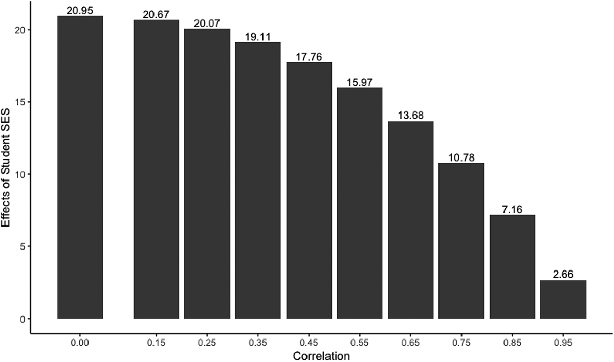
Graphical illustration of changes in relative effects of student SES on science achievement with and without prior measures of science achievement.
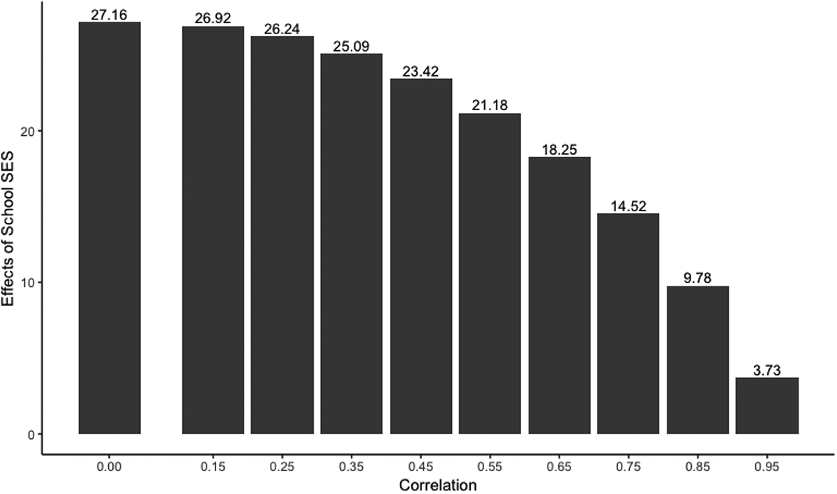
Graphical illustration of changes in relative effects of school SES on science achievement with and without prior measures of science achievement.
Characteristics of Phantom Effects
We have discovered in the present analysis that the phantom effects of student SES and in particular school SES on student science achievement are rather real. In general, these phantom effects can be characterized as such: The stronger the correlation between prior science achievement and (present) science achievement, the greater the chance that the phantom effects occur in terms of student SES and in particular school SES. In the presence of student and school characteristics, a correlation as low as .45 (or even .35) between prior science achievement and (present) science achievement can effectively trigger the phantom effects of school SES. The same correlation meanwhile can also effectively make the effects of student SES sink below the most liberal standard for practical importance (i.e., .20 SD; see Hedges and Hedberg 2007).
Practice of Partial Simulation
Partial simulation provides a new angle to conduct theoretical (simulation) studies of social phenomena. For this type of studies, full simulation has so far been predominately employed to generate data in a laboratory setting which are entirely based on ideal assumptions on conditions and distributions. As far as social sciences are concerned, we argue that data generated in the laboratory setting (i.e., through full simulation) may behave differently from data collected from the real world. We reason that this departure comes from the fact that data generated through full simulation are designed rather than naturally occurred. Although this philosophical issue is certainly open for debate, we argue that partial simulation brings simulation studies of social phenomena closer to the reality. Because of this, the results of partial simulation may appear less strange and more convincing to readers who have little knowledge on full simulation.
Implication for Model Building
We suggest that researchers should be mindful of potential phantom effects in their field. They may use evidence from the research literature to determine the potential correlation between prior and present outcome measures. Based on this estimate, we have provided a way to construct a prior measure in the estimated correlation with the present one. Therefore, researchers do not need to collect but generate data on the prior measure, effectively overcoming the difficulties in collecting certain data. The inclusion of this measure in their model would take phantom effects into consideration and thus improve in a significant way the credibility of their knowledge claim. In fact, we argue that the procedure of partial simulation (i.e., how we created prior science achievement in the present analysis) offers researchers a general way to create variables that are otherwise not available for data analysis. Based on theories and empirical studies, any missing information in data for model specification can be generated by means of partial simulation.
Suggestions for Further Research
As we discussed in the literature review, phantom effects are a largely uncharted field of research. Empirically, many basic research issues remain in the field. Our models are often referred to as the random intercept model because each student-level variable has a fixed slope at the school level, assuming in our case that the effects of (student) SES were the same across schools. One benefit of the random intercept model is that it provides an opportunity to check against Simpson’s paradox. When the SES factor is examined at both student and school levels, Simpson’s paradox may occur, a well-known statistical phenomenon in which a common trend across a number of groups either disappears or reverses once the groups are combined together. We use the first HLM model presented at the very beginning to explain. Because schools share the same SES slope (
We made the decision to fix the (student) SES slope at the school level based on Thum and Bryk (1997) who argued that if the variation across schools in the effects of a student-level variable is not a part of a research question, the student-level variable should be fixed to avoid bias in multilevel modeling. Nonetheless, allowing the (student) SES slope to vary across schools does add a more complex layer of issues to the study of phantom effects. As a result, school-level variables can be used to adjust phantom effects over school characteristics (as in our case) and model the variation in the (student) SES slope. Furthermore, with two random parameters (intercept and SES slope) at the school level, correlation can also be examined between variation in phantom effects and variation in SES slope. Such issues may be important to some researchers and can be pursued with some minor changes to our model specifications.
We employed science achievement as outcome measure in the present analysis. Are there phantom effects associated with student SES and school SES in other outcome measures? We examined school SES as contextual variable in the present analysis. Are there phantom effects associated with other school contextual variables? Methodologically, the present analysis indicates the importance of considering prior student academic achievement when estimating the effects of school context such as school SES. This approach focuses on the missing of important information in model specification. Some researchers have also suggested that phantom effects can occur as a result of measurement errors (see Pokropek 2015). The combination of both approaches may eventually bring researchers to a fuller understanding of phantom effects.
Supplemental Material
Supplemental Material, sj-pdf-1-smr-10.1177_0049124120986195 - A Partial Simulation Study of Phantom Effects in Multilevel Analysis of School Effects: The Case of School Socioeconomic Composition
Supplemental Material, sj-pdf-1-smr-10.1177_0049124120986195 for A Partial Simulation Study of Phantom Effects in Multilevel Analysis of School Effects: The Case of School Socioeconomic Composition by Hao Zhou and Xin Ma in Sociological Methods & Research
Footnotes
Declaration of Conflicting Interests
The author(s) declared no potential conflicts of interest with respect to the research, authorship, and/or publication of this article.
Funding
The author(s) received no financial support for the research, authorship, and/or publication of this article.
Supplemental Material
Supplemental Material for this article is available online.
References
Supplementary Material
Please find the following supplemental material available below.
For Open Access articles published under a Creative Commons License, all supplemental material carries the same license as the article it is associated with.
For non-Open Access articles published, all supplemental material carries a non-exclusive license, and permission requests for re-use of supplemental material or any part of supplemental material shall be sent directly to the copyright owner as specified in the copyright notice associated with the article.