
Abstract
In this article, I present a new multivariate regression model for analyzing outcomes with network dependence. The model is capable to account for two types of outcome dependence including the mean dependence that allows the outcome to depend on selected features of a known dependence network and the error dependence that allows the outcome to be additionally correlated based on patterned connections in the dependence network (e.g., according to whether the ties are asymmetric, mutual, or triadic). For example, when predicting a group of students’ smoking status, the outcome can depend on the students’ positions in their friendship network and also be correlated among friends. I show that analyses ignoring the mean dependence can lead to severe bias in the estimated coefficients while analyses ignoring the error dependence can lead to inefficient inferences and failures in recognizing unmeasured social processes. I compare the new model with related models such as multilevel models, spatial regression models, and exponential random graph models and show their connections and differences. I propose a two-step, feasible generalized least squares estimator to estimate the model that is computationally fast and robust. Simulations show the validity of the new model (and the estimator) while four empirical examples demonstrate its versatility. Associated R package “fglsnet” is available for public use.
In many settings, outcomes tend to be correlated across units of analysis. For example, the academic achievement of students in a classroom or a school may be correlated. The number of friends a person has is likely correlated among the egos and the alters. Perceived risk may be correlated among residents living in the same neighborhood. Regardless of the cause for the correlation, it is important to account for the correlation to make proper statistical estimates and inferences.
Several approaches have been used in the past to account for such correlations. For example, clustered standard errors aim to adjust for the correlation among units in the same cluster. But this approach usually allows only one cluster while multiway clustering is still rarely used (Cameron, Gelbach, and Miller 2011; Zeileis 2006). Another approach is multilevel modeling, which can accommodate multiple clusters (Guo and Zhao 2000; Mustillo and Mustillo 2012; Rabe-Hesketh and Skrondal 2008; Raudenbush and Bryk 2002; Sampson, Raudenbush, and Earls 1997; Snijders and Bosker 2012). But one problem with multilevel modeling (and also clustered standard errors) is that it assumes outcome correlations exist evenly within a cluster, whereas in reality, the outcomes in the same cluster may not be correlated evenly and outcomes may be correlated across clusters.
In this article, I advocate collecting social network data to more accurately represent and model correlated outcomes. Specifically, given a network that depicts the dependence structure across units, I present a new multivariate regression model that can incorporate two types of outcome dependence: (1) the mean dependence that allows the outcome to depend on selected features of the dependence network and (2) the error dependence that allows the outcome to be additionally correlated according to pattered connections in the dependence network. For example, when predicting a group of students’ smoking status, the outcome can depend on the students’ positions in their friendship network and also be correlated among friends. Overall, the two types of dependence help provide more accurate and comprehensive modeling of correlated outcomes, whereas past models usually account for only one type of outcome dependence. In particular, one unique strength of the new model is that it can account for various forms of error dependence based on patterned connections in the dependence network (e.g., according to whether the ties are asymmetric, mutual, or triadic).
I will compare the new model with related models, including multilevel models, spatial regression models, and exponential random graph models (ERGMs), and present both differences and connections between them. I will also show the feasible generalized least square (FGLS) estimator which I propose to estimate the new model is computationally fast and robust.
To show the versatility of the new model, I will present four empirical examples. The first example examines students’ attitude toward smoking in a health intervention and shows the new model helps disentangle the direct treatment effect from the treatment diffusion effect while accounting for extra outcome correlations. This example also shows the new model can be used to account for multilevel correlations besides network-based dependence. The second example examines how social ties and political power affect wealth accumulation among a group of noble Florentine families in the Renaissance period. This example shows how to combine multiple dependence networks to better model error dependence and how the new model differs from traditional spatial regression models. The third example studies advising relations among a group of corporate managers. This example shows that significant error dependence may indicate that important variables have been omitted from the model. The last example examines popularity among students in a Southern U.S. school. It shows that the new model provides a new approach (compared to the ERGMs) to modeling selected network features while also accounting for dependence in tie formation.
The article proceeds as follows. First, I will describe the basic model and show how it can be used to characterize two types of outcome dependence, namely, the mean dependence and the error dependence. To put the new model in context and show its distinct features, I will also compare it with related models. Second, I will introduce the FGLS estimator to estimate the new model and discuss its properties in relation to other estimation methods. Third, I will present simulations to evaluate the performance of the new model and the FGLS estimator. Fourth, I will present four empirical examples for illustration. Finally, I will conclude and discuss possible improvements of the model and the FGLS estimator.
Model and Method
The Basic Model
Assume

In the model,
The error term
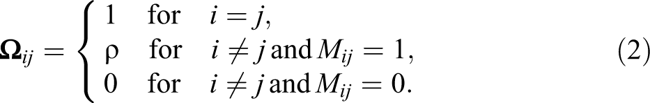
When the dependence network is directed, one approach is to symmetrize it by removing nonmutual ties or by converting nonmutual ties to mutual ones. In the former case,
For a directed dependence network, one can also differentiate the error dependence by relational distance or structural equivalence between units (Leenders 2002) or the types of ties between units as introduced below. Inspired by social network analysis, this article presents three forms of error dependence that represent unmeasured social processes such as hierarchy, reciprocity, and transitivity: (1) asymmetric dependence between units with asymmetric ties in
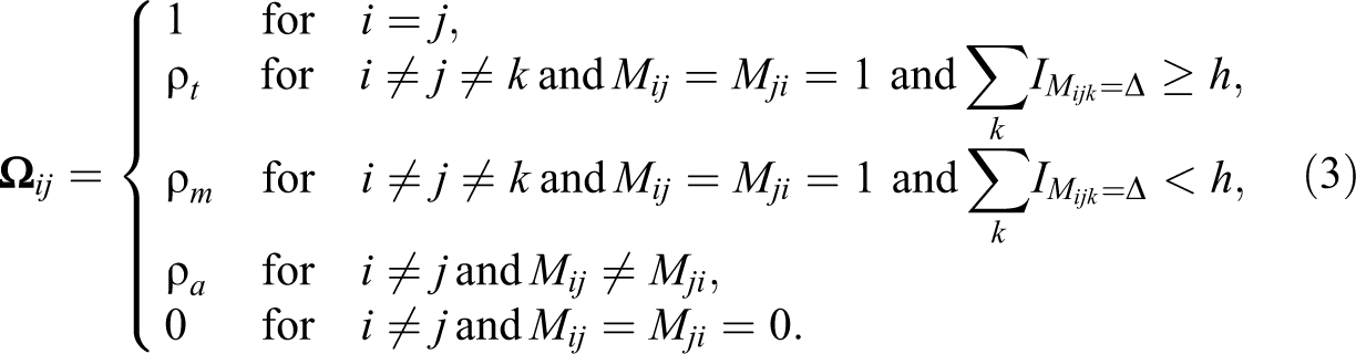
where
In principle, this model can also include error dependence formed upon indirect ties or other kinds of social processes. Some of these have been explored in Leenders (2002), but more variants can be specified following how endogenous tie dependence is specified in ERGMs (Morris, Handcock, and Hunter 2008).
Comparisons With Related Models
Below I compare the new model with related models and point out their differences and connections as well as their relative advantages and disadvantages. Before going into details, I should point out there is an R package “tnam” (not available in the current version of R but available in the R archive) that can account for mean dependence on centrality measures (Leifeld and Cranmer 2017). The package does not account for error dependence.
Spatial regression models
Spatial regression models include several variants. The spatial autoregressive model (i.e., the spatial lag model) aims to account for interdependence among the outcomes of network neighbors (Anselin et al. 1996; O’Malley et al. 2014; O’Malley and Marsden 2008). Suppose

In the spatial autocorrelation model (also called the spatial error model), the error terms are assumed to be spatially correlated,


The spatial autoregressive and autocorrelation model combines the spatial autoregressive model and the spatial autocorrelation model by including both direct outcome dependence and error dependence. Note that the two types of dependence do not have to be based on the same dependence network.


There are three major differences between the new model and the spatial regression models. First, the types of network dependence that are modeled are different. The spatial autoregressive and autocorrelation model (the most comprehensive version of the spatial regression models) can account for autoregressive (outcome) dependence and error dependence while the new model can account for mean dependence (which is usually absent in the spatial regression models) and error dependence. In the spatial regression models with a spatial autoregressive process, the parameter
Second, the error dependence structure is specified differently. In the spatial regression models with an autocorrelation process, the error terms are usually assumed to be
Finally, the estimation methods are different. The spatial regression models are typically estimated by the ordinary least squares (OLS) combined with the maximum likelihood estimation. The new model is estimated by the FGLS, which is computationally faster and more robust.
Despite the differences, it is possible to combine the two types of models. For example, one may revise the spatial autoregressive and autocorrelation model by including the mean dependence and varying error dependence as how it is specified in the new model.
ERGMs
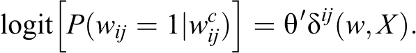
ERGMs aim to model network formation (Hunter and Handcock 2006; Robins et al. 2007; Snijders et al. 2006; Wasserman and Faust 1994). The probability of observing a network w is assumed to be
ERGMs are typically estimated by Monte Carlo Markov chains, except in the pseudolikelihood estimation (Strauss and Ikeda 1990; Wasserman and Pattison 1996; Yamaguchi 2003). As a result, the estimation process is usually computationally intensive and slow, especially for big networks.
Unlike ERGMs, the new model assumes the dependence network is given and uses it to model the correlations in another outcome. That said, the different forms of error dependence presented in this article resemble how endogenous tie formation processes are modeled in ERGMs. Hence, other forms of tie dependence that have been studied in ERGMs may be adopted in the new model to configure the error dependence structure (Morris et al. 2008).
The new model can be used to model selected network features (e.g., indegree) rather than the network itself. Because of the resemblance between the error dependence structure and endogenous tie formation processes, the estimated error dependence structure (e.g., mutual and triadic correlations) may be informative of corresponding endogenous tie formation processes (e.g., reciprocity and transitivity). Hence, the new model may serve as an alternative but computationally faster approach to understanding endogenous tie formation processes.
Estimation
I utilize an FGLS estimator to estimate the model (Greene 2008). This is a two-step procedure. First, I estimate the model by OLS and use the residuals of network neighbors to estimate the correlation coefficient


where
The correlation coefficient

where
To make inferences on the estimated error correlation coefficients, one may use the Wald test in the corresponding residual regressions. For example, for equation (11), one can simply use the estimate and the standard error to conduct hypothesis testing. Another approach is to use the Breusch–Godfrey test (Breusch 1978; Godfrey 1978) that is typically used for assessing serial correlations in panel data. The Breusch–Godfrey test shows that
The downside of these two approaches is that they ignore heteroscedasticity (when the variances of the error terms in the residual regression differ across units) and clustering (when ego units are connected to multiple alters). To address this issue, one may use standard errors clustered by ego units (Cameron and Miller 2015) or even by egos and alters jointly. To note, if the number of clusters is relatively small compared to the number of units within clusters, conventional clustered standard errors may not work as effectively (Hansen 2007).
Resampling methods can also be useful. One is bootstrapping, namely, resample the residuals with replacement (or even within ego blocks), and refit the residual regression many times. Then, the estimates can be used to form a sampling distribution to construct standard errors and perform hypothesis testing. Another approach is the permutation test. Basically, one resamples the predictor without replacement and refits the residual regression many times. The resulting estimates can form a null distribution of no error dependence to benchmark against the originally estimated correlations.
However, my simulations and prior research (Dow, Burton, and White 1982; Langford, Schwertman, and Owens 2001) show that all these procedures hold only approximately. My simulations further show that the inferences behave relatively well under two conditions: (1) the true correlation coefficients are small and (2) the dependence network is sparse (Leung 2020). To note, when the true correlation coefficient
One may use the Fisher’s (1921) transformation method to test the difference between correlation coefficients. Namely, for two error correlation coefficients, one can obtain a p value based on the z-score
The model may be simply estimated by OLS. As is known in the literature, the OLS will be unbiased and consistent (Greene 2008). But there are two drawbacks of doing so. First, if the multivariate model is true, then in large samples, the OLS standard errors will be larger and inefficient. Note that in small samples, there is no guarantee that the FGLS will be more efficient than the OLS. Second, sometimes the error dependence may be the center of interest that can inform important social processes, but using the OLS will certainly ignore this.
Sometimes, the covariance matrix
Additional Comments
Below I discuss possible extensions of the new model and address concerns on its assumptions. First, the model may be extended to incorporate different types of dependence networks. (1) Weighted dependence. In a weighted dependence network, the tie values are continuous or categorical. One option is to binarize the network and then apply the methods outlined above. Another option is to use the weighted versions of asymmetric, mutual, and triadic dependence. For example, mutual dependence occurs when the tie values between two units are equal or close. Triadic dependence happens when two units have mutual dependence not only between themselves but also with other units. In addition, weighted centrality measures (Butts 2008) can be easily included in the regression to represent the mean dependence. (2) Multiplex dependence. When multiple dependence networks are available, one may create a single binary dependence network in which there is a tie between two units as long as there is a tie between them in any of the original networks. Alternatively, one may combine the multiple networks into a weighted one. To account for the mean dependence, one can use centrality measures in the original dependence networks or in the combined network. (3) Multilevel dependence. Outcome correlations may also occur in nested groups such as classes, grades, and schools. The first empirical example below will show how the new model can account for such multilevel dependence and network dependence simultaneously.
Second, the model assumptions may be relaxed in future development. (1) The model assumes the error dependence structure is known. However, this may not be the case. Like for solving a model selection problem, I suggest using theories to guide the specification of the error dependence structure. For directed dependence networks, one may start with more complicated forms of error dependence and gradually reduce it to simpler forms. For example, if triadic dependence is found to be statistically insignificant from mutual dependence, then the two forms of dependence may be combined. If the error dependence structure is misspecified, the FGLS estimate of the error dependence structure will be biased. Although the estimates in the outcome model will still be unbiased, their standard errors and the associated testing and inferences may be incorrect. This can also lead to that FGLS is less efficient than OLS.
In this article, I specify only three forms of error dependence. Future work may investigate other forms of error dependence such as cyclic or cliquish dependence that involves more units or indirectly connected units. Since the number of observations in the covariance matrix grows very quickly as n increases, there usually is a sufficient degree of freedom to estimate complex forms of error dependence. But for model conciseness, a few forms of error dependence usually suffice. Of course, for small networks, one should be careful not to specify too many error correlations.
(2) The model assumes that one unit can only be in one type of error dependence and prioritizes triadic dependence over mutual dependence and further over asymmetric dependence. For example, when a tie falls into both mutual and triadic error dependence, the model assigns the tie to triadic dependence. Future work may change such assignment.
(3) The dependence network may depend on the outcome which will cause a reverse causality issue. For example, suppose the outcome is happiness at school and the dependence network is friendship network. While friendship centrality can affect happiness, happiness may also affect centrality. One method that can help identify the causal effect of centrality is by using instrumental variables namely, variables that can only affect happiness indirectly through their effects on centrality (e.g., some random assignment of classroom seats). More generally, through a two-stage method, one first uses the instrumental variables (and exogenous covariates) to predict the network measures representing the mean dependence and then uses the predicted network measures in the outcome model to estimate the causal effect of the mean dependence (Wooldridge 2010).
Simulations
Error Dependence Only
The first set of simulations focus on examining patterns of error dependence. The number of units is set at 1,000. Half of the units are randomly assigned to a binary treatment (


Panel A in Table 1 shows the simulation results. First, the FGLS provides unbiased estimates for both the covariate coefficients and the error correlation coefficient. Second, the mean standard errors of the estimates are very close to the standard deviations of the estimates. Hence, statistical inferences based on the FGLS are expected to be accurate. Indeed, the coverage rates of the 95 percent confidence intervals are all right at or around the target level.
Simulations With Error Dependence Only.
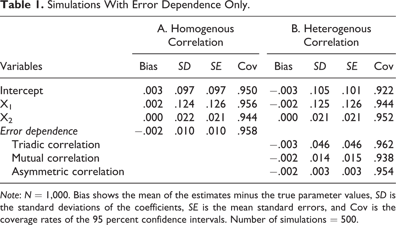
Note: N = 1,000. Bias shows the mean of the estimates minus the true parameter values, SD is the standard deviations of the coefficients, SE is the mean standard errors, and Cov is the coverage rates of the 95 percent confidence intervals. Number of simulations = 500.
I also conducted additional simulations (shown in Online Appendix Tables A1 and A2 [which can be found at http://smr.sagepub.com/supplemental/]) to compare OLS and FGLS. For the estimated coefficients (except the intercept) in the outcome model, the FGLS is slightly more efficient than the OLS. There is actually no bias in the OLS estimates, and the statistical inferences are also approximately correct. But the OLS estimates ignore the error correlation that may indicate some significant aspect of the data generation process.
In the second set of simulations, I allow the error correlation coefficients to vary by the forms of error dependence. I specify the correlation coefficients for triadic, mutual, and asymmetric error dependence at 0.02, 0.01, and 0.005, respectively. The ties in the dependence network (
Panel B in Table 1 shows the simulation results. Once again, the FGLS provides unbiased estimates of the coefficients and also proper statistical inferences on the estimates. The average standard errors of the estimates are close to the actual standard deviations of the estimates, and the coverage rates of the 95 percent confidence intervals are all near to the nominal level.
Both Error Dependence and Mean Dependence
In these simulations, I allow selected features of the dependence network to affect the outcomes. To mimic that some units are more likely to correlate with others, the probabilities for treated units (

The mean dependence is represented by
Table 2 shows the simulation results. The most striking finding is that when the mean dependence is ignored in the regressions, the estimates on all parameters have dramatic bias. The estimated coefficients for the covariates and the error correlations are both way off from the target values. The standard errors are also way bigger than the standard deviations. As a result, the coverage rates of the 95 percent confidence intervals all miss the target level.
Simulations With Both Error and Mean Dependence.

Note: N = 1,000. Bias shows the mean of the estimates minus the true parameter values, SD is the standard deviations of the coefficients, SE is the mean standard errors, and Cov is the coverage rates of the 95 percent confidence intervals. Number of simulations = 500.
In contrast, the regressions including the mean dependence provide proper estimates. The estimated coefficients for both the covariates and the error correlations are close to the target values. The average standard errors of the estimates are also close to the standard deviations of the estimated coefficients. The coverage rates of the 95 percent CIs are all around the target level. Overall, the simulation results show the importance of accounting for both the mean dependence and the error dependence and the capability of the new model to achieve this.
Examples
Estimating Causal Treatment Effect With Treatment Diffusion
The data for this example are from a smoking prevention intervention the author conducted in 2010–2011 in six middle schools in China. Selected classrooms from each school were assigned to one of four conditions, including control, random intervention targeting random students, central intervention targeting central students who could connect to most other classmates via friendship ties (Borgatti 2006), and group intervention targeting students and their closest friends in their classroom. In each treated classroom, a quarter of students were selected for the intervention. The intervention included distributing brochures to and holding a workshop for the treated students. In total, 3,445 students participated in the experiment.
All students took part in two surveys: one before the intervention and one after. In both surveys, students were asked to respond to 10 questions on attitude toward smoking. Each response not supporting smoking scores five points. The aggregate score for each student is used to measure the student’s attitude toward smoking. The goal is to study whether the intervention has an effect of enhancing treated students’ attitude against smoking. One problem is that students may share the intervention information with others. As such, simply comparing the treated with the untreated may provide a biased estimate of the treatment effect. In addition, students’ attitude may be correlated among those who have shared the intervention information or who are friends because of their communications or sharing unobserved common traits. The traditional way to model the data would be to use a multilevel model that assumes equal correlations among students in the same class, the same grade, or the same school. This assumption is likely inaccurate in reality.
In contrast, the new model provides a more effective way to model the data. Specifically, I use a lagged dependent variable model to analyze the data with the attitude score at the outcome survey as the dependent variable and the baseline attitude score as one of the covariates. Other baseline covariates include sex (1 = boy; 0 = girl), smoking status (1 = yes; 0 = no), academic ranking (1 = ranked top 10 in the class; 0 = otherwise), personality (1 = optimistic; 0 = not optimistic), family economic condition (1 = good; 0 = not good), friendship indegree (i.e., number of incoming friendship ties), friendship outdegree (i.e., number of outgoing friendship ties), and indicators for missing the outcome survey and for grades and schools. To account for nonrandom treatment assignment, I also control for students’ propensity score for receiving the intervention, where I use a logit model to predict the propensity of a student receiving the intervention based on covariates (see Online Appendix Table A3 [which can be found at http://smr.sagepub.com/supplemental/]). In the outcome survey, students were asked to report from which schoolmates they have seen and read the prevention brochure. The responses are used to construct a treatment diffusion network in each school.
I specified three models. In the first one, the error terms are correlated among treatment diffusion partners. I distinguish triadic, mutual, and asymmetric error dependence. In the second specification, to tease out the direct treatment effect from the treatment diffusion effects, I additionally control for two measures based on the treatment diffusion network: (1) information outdegree (i.e., number of students from whom a student has obtained the intervention information) and (2) information indegree (i.e., number of students with whom a student has shared the intervention information). In the third specification, the error terms are correlated between treatment diffusion partners as well as friends.

Table 3 shows the results. (1) The baseline attitude is positively and significantly correlated with the outcome attitude (
Estimating Causal Treatment Effect on Attitude With Treatment Diffusion.
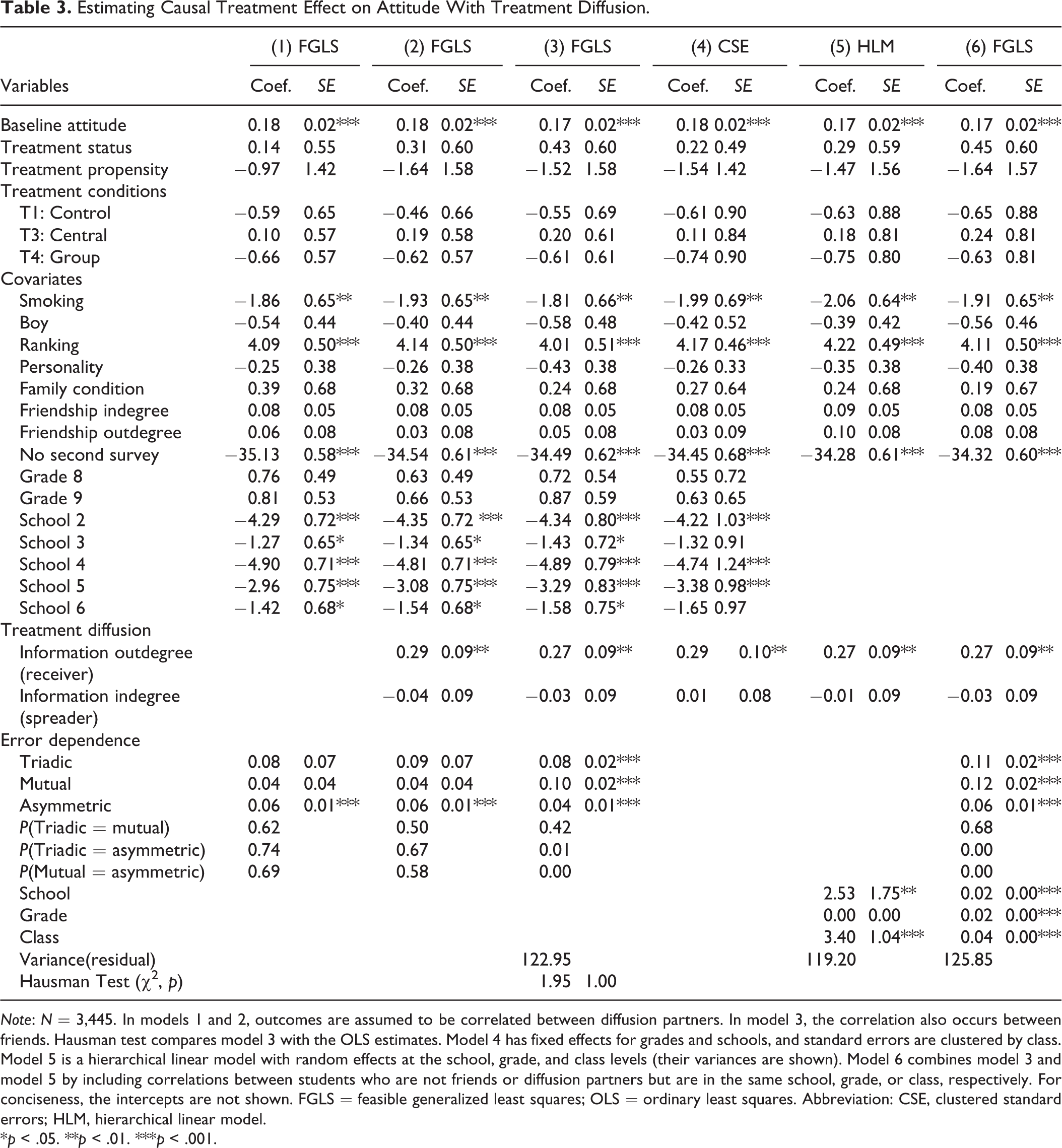
Note: N = 3,445. In models 1 and 2, outcomes are assumed to be correlated between diffusion partners. In model 3, the correlation also occurs between friends. Hausman test compares model 3 with the OLS estimates. Model 4 has fixed effects for grades and schools, and standard errors are clustered by class. Model 5 is a hierarchical linear model with random effects at the school, grade, and class levels (their variances are shown). Model 6 combines model 3 and model 5 by including correlations between students who are not friends or diffusion partners but are in the same school, grade, or class, respectively. For conciseness, the intercepts are not shown. FGLS = feasible generalized least squares; OLS = ordinary least squares. Abbreviation: CSE, clustered standard errors; HLM, hierarchical linear model.
*p < .05. **p < .01. ***p < .001.
To compare the new model with traditional models, I also fit two other models. The first one (shown in model 4 of Table 3) has fixed effects at the grade and school levels and standard errors clustered at the class level. The second one is a multilevel model (model 5 of Table 3) with random effects at the school, grade, and class levels, respectively. I will compare models 4 and 5 with model 3 to illustrate the major differences. First, the estimated coefficients and their standard errors differ across the models. The differences can go in either direction, being larger or smaller, and that the differences in the estimated coefficients and their standard errors do not necessarily go in the same direction at the same time. None of the differences seem to be statistically significant. But we cannot generalize the results to other cases. It could be the case that the differences happen to be large enough to alter statistical inferences. For example, the coefficients for academic ranking are larger in both models 4 and 5 while the standard errors are both smaller. As a result, it is more likely to reject the null hypothesis in either of these two models. Second, the interpretations of the models are different. Model 4 assumes that students’ attitude is correlated within classroom only, and the correlation is the same between any two students who are in the same classroom. This seems unrealistic either for friends who are in the same classroom or for friends who are in different classrooms but the same school. Model 5 assumes that students’ attitude is correlated by school, grade, and class, respectively, and the correlation is the same for any two students who are in the same cluster. For example, model 5 shows that students’ attitude in the same school and the same class has a covariance of 2.53 (
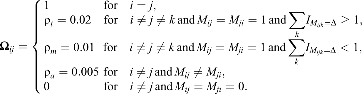
One way to incorporate features of the multilevel model into the new model is to add correlation coefficients to represent correlations between students who are not friends or diffusion partners but are in the same school, grade, or classroom. See Figure 1 for an illustration. In model 6 of Table 3, I add three additional correlation coefficients to represent correlations between nonfriends or nondiffusion partners who are in the same classroom, in the same grade but a different classroom, and in a different grade but the same school, respectively. The results remain largely the same as in model 3. But patterns of the error dependence are quite different. Model 6 shows that the attitudes of friends or diffusion partners are significantly correlated (all
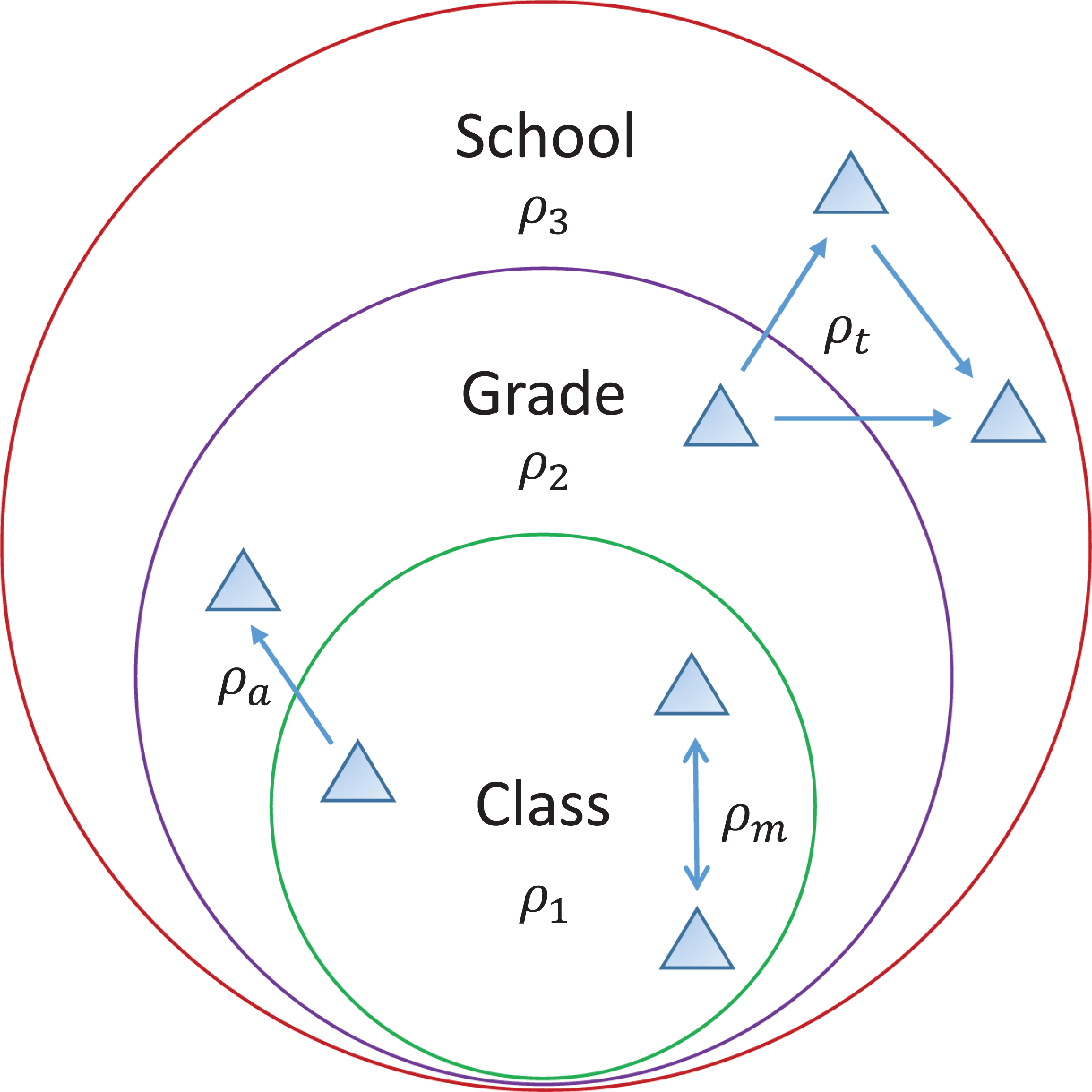
The new model with various forms of error dependence. Note: In this example, the new model includes correlation coefficients that can account for triadic, mutual, and asymmetric error dependence (
The new model can be applied to modeling other similar outcomes as well for example, students’ test scores. The test scores can depend on students’ positions in their friendship network (e.g., because central students may get more help from peers and teachers). The test scores can also be correlated among friends as well as among nonfriend students who are in the same classroom, the same grade, or the same school.
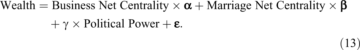
Wealth and Network Centrality Among Florentine Families
The data for this example are about wealth and social networks among 16 Florentine families in the Renaissance period collected by John Padgett (Padgett and Ansell 1993). The goal is to study whether family wealth is determined by the political power and the network centrality held by the families and whether wealth is additionally correlated among families with social ties. The data do not allow one to pin down causality, but are useful for illustrating how to incorporate multiple dependence networks and comparing the new model with spatial regression models.
The dependent variable is family net wealth in 1,427 (in thousands of lira). Political power is measured by the number of seats on the civic council held by the families. The two social networks are undirected, including business ties and marriages ties among the 16 families. From the business network, I extract indegree centrality and eigenvector centrality. From the marriage network, I extract indegree centrality, betweenness centrality, and eigenvector centrality. Indegreee measures the number of ties a family has in a network. Betweenness centrality measures the brokerage power of a family, and eigenvector centrality measures the extent to which a family is connected to important others (Wasserman and Faust 1994). To note, in general, one should be careful not to include multiple centrality measures in the same model simultaneously because of potential multicollinearity among the centrality measures.
I specified two models to predict family wealth. In the first model, the dependence network is only based on the business network. Thus, the wealth of two families are correlated if they have a business tie. Because wealth can also spread across families by marriage, in the second model, I also allow family wealth to be correlated if two families have a marriage tie. Therefore, two families’ wealth are correlated if they have a tie in either network. In the second model, I also distinguish two forms of error dependence: triadic versus mutual. Because the two dependence networks are undirected, there is no asymmetric error dependence.
Models 1 and 2 in Table 4 show the results. In both models, the more business ties a family has, the wealthier the family is (
Wealth and Network Centrality Among Florentine Families.
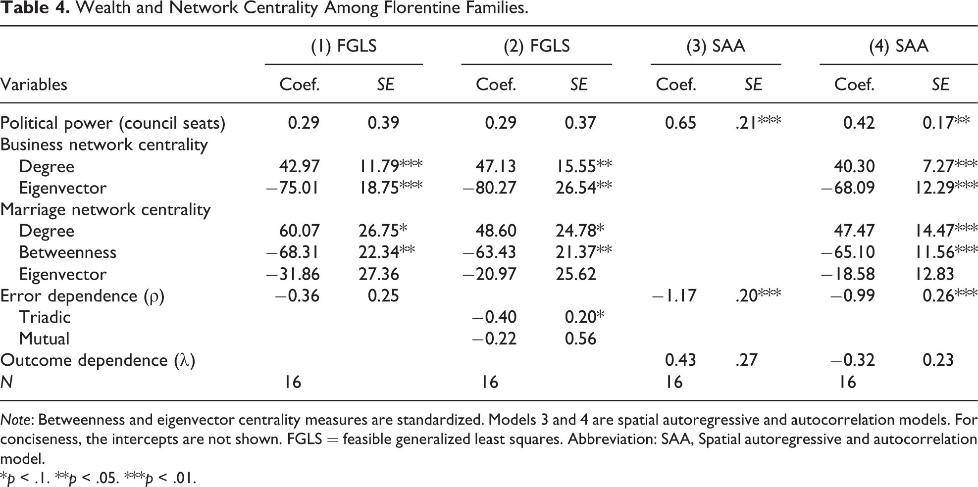
Note: Betweenness and eigenvector centrality measures are standardized. Models 3 and 4 are spatial autoregressive and autocorrelation models. For conciseness, the intercepts are not shown. FGLS = feasible generalized least squares. Abbreviation: SAA, Spatial autoregressive and autocorrelation model.
*p < .1. **p < .05. ***p < .01.
The error dependence is not statistically significant, even at the 10 percent level in the first model, whereas in the second model, the triadic error dependence (but not the mutual error dependence) is statistically significant at the 10 percent level. Hence, the multiplex dependence network captures the unobserved wealth correlation across the families better. The error correlations are negative, which may be a result of disassortative mixing by which families with different amounts of wealth are more likely to be connected through social ties.
For comparison, I also fit two spatial autoregressive and autocorrelation models. The weight matrix
Are Central Managers More Likely to Be Sought for Advice?
The third example aims to show that the error dependence may be an indication of the effects of omitted variables. The data were collected by Krackhardt (1987). It includes two directed social networks among 21 managers in a company. In the advising network, there is a tie from A to B if A has asked B for advice. In the friendship network, there is a tie from A to B if A has nominated B as a friend. Managers’ attributes used in this article include the length of tenure in the company, level in the corporate hierarchy (1 = manager, 2 = vice president, and 3 = CEO), and departmental affiliation (1–4 with CEO being recoded into 1).
The goal of this example is to study whether managers with many friends are more likely to be sought after for advice. I treat indegree in the advising network as the dependent variable and indegree in the friendship network as one of the predictors. Past research has also shown that people with brokerage positions are more likely to have innovative ideas (Burt 2004). Thus, I also include betweenness centrality in the friendship network as a predictor. I specify two models. In the first model, I use tenure, level, and friendship indegree and betweenness to predict the advising indegree. The error terms are assumed to be correlated among friends. In the second model, I additionally control for the managers’ departmental affiliations.

Table 5 presents the results. The first model shows that as compared to the CEO, the vice presidents are significantly more likely to provide advice to others (
Advising and Friendship Among Corporate Managers.
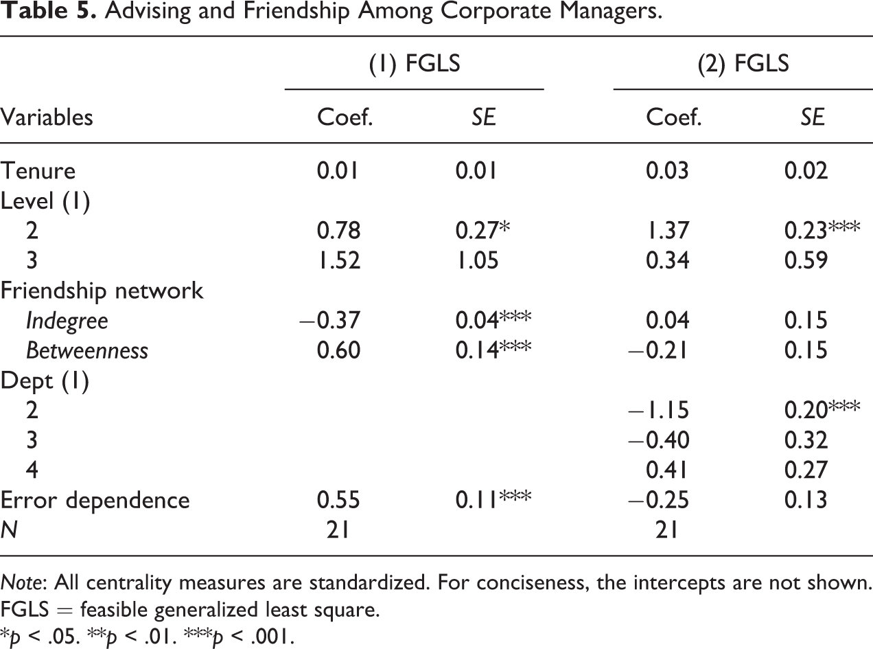
Note: All centrality measures are standardized. For conciseness, the intercepts are not shown. FGLS = feasible generalized least square.
*p < .05. **p < .01. ***p < .001.
Predicting Popularity Among High School Students
The data for the last example include an undirected friendship network of 1,461 students in a U.S. high school and student covariates such as sex (0 = female; 1 = male), race (0 = black; 1 = white; 2 = others), and grade (7–12; Goodreau et al. 2008; Handcock et al. 2003; Resnick et al. 1997). The goal of this example is to predict students’ indegree and closeness centrality in the friendship network, respectively. The error terms are assumed to be correlated among friends, and mutual and triadic error dependence are differentiated. The specification of the error dependence allows the new model to shed lights on endogenous tie formation processes.
Models 1 in Table 6 predicts friendship indegree. The results show that female students, white students, and students in the eighth grade have significantly more friends than the reference groups (all
Predicting Popularity Among School Students.
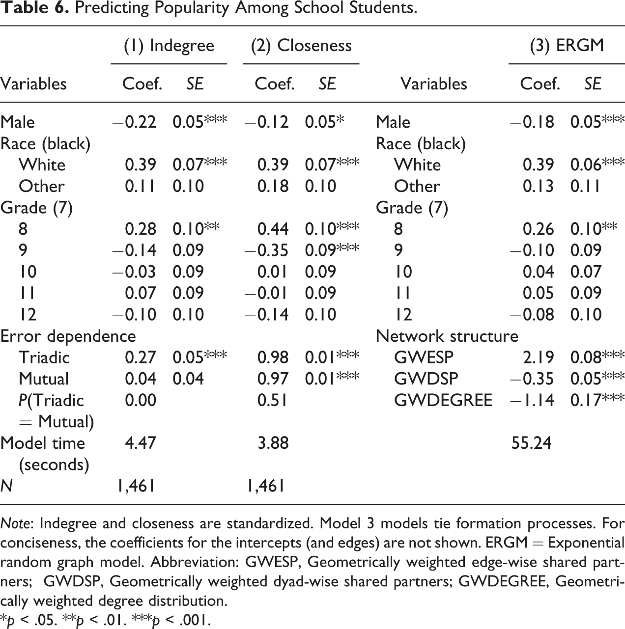
Note: Indegree and closeness are standardized. Model 3 models tie formation processes. For conciseness, the coefficients for the intercepts (and edges) are not shown. ERGM = Exponential random graph model. Abbreviation: GWESP, Geometrically weighted edge-wise shared partners; GWDSP, Geometrically weighted dyad-wise shared partners; GWDEGREE, Geometrically weighted degree distribution.
*p < .05. **p < .01. ***p < .001.
Model 2 in Table 6 predicts closeness centrality. Female students, white students, and students in the eighth grade are socially closer to peers in their school than their counterparts are (all
Model 3 in Table 6 shows the results of an ERGM that is fit on the friendship network. Similar to model 1, this model shows that female students, white students, and students in the eighth grade have significantly more friends than their counterparts (all
In short, the new model is able to reveal the same set of covariates that significantly predict student popularity as in the ERGM. The significant triadic error dependence in model 1 is also indicative of friendship transitivity. However, we should also be aware that the new model and ERGMs have some fundamental differences. The new model is developed to model selected macro features of a social network while ERGMs specifically aim at modeling micro tie formation processes. The former takes a vector as the dependent variable while the latter a whole network. The new model is computationally faster and more stable but lacks the ERGM’s capability of modeling covariate effects on incoming and outgoing ties simultaneously (for directed networks) and more nuanced endogenous tie formation processes. Nonetheless, the new model and ERGMs can be complementary to one another. When a vector of network feature instead of the whole network is more suitable as the dependent variable, the new model is more useful.
Conclusion and Discussion
In this study, I introduce a new multivariate regression model for analyzing outcomes with network dependence. I highlight the importance of accounting for both mean dependence and error dependence. Ignoring mean dependence may lead to severe bias in the estimated covariate effects. Ignoring error dependence does not impair the consistency of the estimated covariate effects. But inferences on the estimates may be less efficient, and extra outcome correlations are ignored that may be informative of important data generation processes.
I proposed an FGLS estimator to estimate the new model. The estimator is shown to be computationally fast and robust. I also show the distinct features of the new model in comparison to previous models such as multilevel models, spatial regression models, and ERGMs. In particular, one may view the current model as a modification of the spatial error model with the error structure in the current model being specified in a more intuitive and flexible way. To reiterate, the new model is not meant to replace prior models as they have different strengths depending on the context.
Simulation results suggest that the new model and method provide unbiased estimates and correct inferences on both the covariate effects and the error dependence. The four empirical examples illustrate the wide applicability of the new model. To facilitate future research, I have incorporated the model and method into an R package “fglsnet” for public use (see the author’s website for more information).
Of course, the new model and method can be extended in several ways. I have discussed some of the extensions when introducing the model above. Here I I would like to point out two more extensions. First, more work is needed to check the robustness and consistency of the model and method in different scenarios. Second, sometimes data on the dependence network may be unavailable. In that case, one may need to locate data that can approximate the dependence network. For example, one may use friendship network to approximate treatment diffusion network assuming diffusion tends to follow friendship ties. One can also use the latent space model (Hoff, Raftery, and Handcock 2002) to impute the dependence network based on similarity between units.
Supplemental Material
Supplemental Material, sj-docx-1-smr-10.1177_00491241211031263 - A Tale of Twin Dependence: A New Multivariate Regression Model and an FGLS Estimator for Analyzing Outcomes With Network Dependence
Supplemental Material, sj-docx-1-smr-10.1177_00491241211031263 for A Tale of Twin Dependence: A New Multivariate Regression Model and an FGLS Estimator for Analyzing Outcomes With Network Dependence by Weihua An in Sociological Methods & Research
Footnotes
Acknowledgments
The author would like to thank the Graduate School of Arts and Sciences, the Multidisciplinary Program in Inequality and Social Policy, the Fairbank Center for Chinese Studies, and the Institute for Quantitative Social Science, all at Harvard University, for the financial support for data collection. The author would also like to thank the reviewers for their helpful comments.
Declaration of Conflicting Interests
The author(s) declared no potential conflicts of interest with respect to the research, authorship, and/or publication of this article.
Funding
The author(s) received no financial support for the research, authorship, and/or publication of this article.
Supplemental Material
The supplemental material for this article is available online.
References
Supplementary Material
Please find the following supplemental material available below.
For Open Access articles published under a Creative Commons License, all supplemental material carries the same license as the article it is associated with.
For non-Open Access articles published, all supplemental material carries a non-exclusive license, and permission requests for re-use of supplemental material or any part of supplemental material shall be sent directly to the copyright owner as specified in the copyright notice associated with the article.