Mapping Social Change: A Unified Framework for Temporal Clustering

Abstract

Analyzing social change requires detecting patterns of continuity and difference over time. While time-series clustering offers a valuable approach, existing techniques are often limited by assuming fixed cluster definitions and static assignments of entities to clusters. To address these limitations, we introduce a unified framework of temporal clustering methods that allows for both dynamic cluster definitions and the transition of entities between clusters, generalizing and extending previous work. We also provide new algorithms for this dynamic clustering that optimize global objectives, with optional constraints on the transitions of entities across clusters. This framework expands the methodological toolkit for analyzing social change, and we provide guidelines for its application. We illustrate our approach with three case studies: polarization of social and political attitudes across U.S. states; cross-national cultural change; and the evolution of neighborhood business patterns. We conclude with directions for further research.

Keywords

temporal clustering machine learning time-series analysis social change neighborhood change

Introduction

Understanding social change—the aggregate shift in characteristics of units like neighborhoods, countries, or states over time—is a central task in sociology and related fields (Fosse 2023a, 2023b; Fosse and Winship 2023; Silver et al. 2022a; Silver and Silva 2021, 2023; Silver et al. 2022b).¹ Recent studies have examined such change in various areas, such as political party identification (Fosse and Winship 2023), gender attitudes (Meagher and Shu 2019), and verbal ability (Fosse 2023c), across a range of units, such as societies, organizations, and neighborhoods (Dias and Silver 2021). However, analyzing social change is challenging because it requires identifying patterns of continuity and difference across many units, each measured on multiple features, while the broader social context itself may be shifting (Fosse 2023a).

Clustering methods are well suited for analyzing complex, multidimensional patterns of social change. By grouping units on many features at once, they can reveal important underlying patterns, even when relationships are nonlinear and heterogeneous. $K$ -means clustering (Fonseca 2013), a simple and efficient approach, remains the most widely used method in sociology, and also serves as the basis for more advanced clustering methods. As a center-based clustering technique, $K$ -means identifies a set of $K$ optimal points in the feature space that serve as cluster centers, where $K$ is chosen based on the researcher’s specific needs and domain knowledge.² The goal is to create groups that are internally coherent and distinct from other groups. The cluster center represents the typical profile for that group, which is its cluster definition. An entity’s assignment to a particular group is its cluster label.

While conventional clustering methods are useful, they typically group entities based on their similarities without considering their temporal sequencing. The analysis of social change, however, requires incorporating a temporal dimension. This extension leads to temporal clustering: grouping complex entities based on their trajectories over time, such as cultural values of countries, voting patterns in U.S. states, or business compositions of neighborhoods.³ This paper presents a unified framework for temporal clustering that expands the methods for analyzing social change. Our framework organizes existing approaches, while introducing new ones.

Our framework is structured around two key dimensions: (a) cluster definitions and (b) cluster labels. Cluster definitions (the characteristics that define a group) can be either static or dynamic. For example, the definition of a “high” fertility country or a “red” state may evolve. Second, cluster labels (the assignment of entities to groups) can also be static or dynamic. A country might move from a “high” to a “low” fertility cluster, or a U.S. state might move from a “red” cluster to a “blue” cluster. Combining these two dimensions creates a typology that organizes existing temporal clustering methods (e.g., Aghabozorgi et al. 2015; Delmelle 2016; Liao 2005), and identifies new ones, including those where both labels and definitions change simultaneously.

The remainder of this paper proceeds as follows. We first present our unified framework and the four classes of temporal clustering methods it subsumes. We then detail the methodology, from the underlying clustering objectives and optimization algorithms⁴ to practical considerations for implementation. Next, we illustrate our framework with three case studies: state-level political polarization in the United States, cross-national cultural change, and the evolution of business establishments in Chicago neighborhoods. We conclude by summarizing key contributions and suggesting directions for further research.

Unified Framework for Temporal Clustering

In this section, we present the proposed unified framework for temporal clustering. The foundation of the proposed framework is built on top of center-based clustering, whose intuition was discussed in the previous section. In this context, a cluster definition refers to the set of characteristics that describes the typical profile of a cluster that is shared among all entities in this cluster (e.g., a cluster with countries that share the “increasing fertility over years” trend), which can be directly inferred from the center of each cluster. The cluster label denotes the assignment of each entity to a specific cluster at a given time (e.g., a state being labeled as “red” or “blue”).

However, existing clustering approaches are often limited by two critical assumptions. First, many methods assume fixed cluster definitions, such that the characteristics defining each group remain constant over time. This assumption is problematic because the substantive meaning of categories can shift significantly: for example, the threshold for “high fertility” declined substantially during the late twentieth century, and the characteristics distinguishing “red” and “blue” U.S. states have evolved alongside changes in political polarization. This can result either in incorrect cluster definitions, where evolving temporal trends are obscured by a static definition, or in misaligned cluster assignments, such that a high-fertility country is incorrectly grouped into a low-fertility cluster as its fertility rate declines over time, making it more similar to the static definition of low fertility.

Second, conventional methods frequently impose static cluster membership, meaning that once an entity is assigned a cluster label, it cannot transition even if its characteristics change. This assumption fails to capture important dynamics, such as states like Texas and Oklahoma shifting their political alignments across decades, or countries moving toward greater secularization in global value surveys. As we later demonstrate in case studies, applying methods that assume fixed definitions and cluster labels would obscure meaningful shifts or exaggerate stability where none exists. Without accounting for the possibility that both the definitions of clusters and the membership of entities may change, traditional clustering methods risk producing misleading or incomplete representations of social change.

To address these limitations, we introduce a unified framework for temporal clustering that systematically incorporates dynamic cluster definitions and dynamic entity memberships. The framework expands the methodological toolkit available for analyzing how entities evolve across time and space. We present this unified framework based on two key dimensions. This framework is shown in Table 1. The rows of the table represent the dynamism of cluster definitions, while the columns of the table indicate the dynamism of the cluster labels or the composition of the clusters. For the cluster definitions, the key question is: Is the definition of the cluster allowed to change over time? For example, with respect to political polarization, does what it means to be a “blue” versus “red” state change over time? This might occur, for example, if being a “red” state initially depends on mass social attitudes but then becomes more of a function of party identification. For the cluster labels, the key question is: Are the cluster labels of the entities allowed to change over time? For example, is a state such as Ohio allowed to move from a “blue” state cluster to a “red” state cluster, or must Ohio always be classified as either “red” or “blue”? This framework yields four classes of temporal clustering methods, as illustrated in Table 1.

Table 1.

Temporal clustering methods: Definitions and use cases The table presents four main temporal clustering methods categorized by two dimensions: the dynamism of cluster definitions (rows) and the dynamism of cluster labels (columns). Examples are based on different assumptions of the definition and composition of “red” and “blue” states in the U.S. $L$ is a hyperparameter that denotes the maximum number of allowable changes in the cluster labels.

Cluster Labels
		Static	Dynamic
Cluster Definition	Static	Static Clustering (SC) $L = 0$ Both cluster definitions and labels are static. This approach ignores time entirely. Example: Grouping states into “blue” and “red” clusters under the assumption that the definition of “blue” and “red” states do not change and that no state moves from being a “red” state to a “blue” state (or vice versa).	Sequence Label Analysis (SLA) $1 \leq L < All Possible Changes$ (bounded) Static cluster definitions with a restricted number of entities allowed to move across clusters. Example: Grouping states into “blue” and “red” clusters under the assumption that the definition of “blue” and “red” states do not change, but allowing a specified number of states to move from being a “red” state to a “blue” state (or vice versa). Useful for highlighting atypical and/or important movements of states across clusters.	$L \geq All Possible Changes$ (unbounded) Static cluster definitions with all entities allowed to move across clusters. Example: Grouping states into “blue” and “red” clusters under the assumption that the definition of “blue” and “red” states do not change, but allowing all states to move from being a “red” state to a “blue” state (or vice versa).
	Dynamic	Time-Series Clustering (TSC) $L = 0$ Dynamic cluster definitions but fixed cluster labels. If only one cluster is assumed, then this simplifies to a conventional year-by-year (period-based) analysis.Example: Grouping states into “blue” and “red” clusters while allowing the definition of “blue” and “red” states to evolve, but assuming that no state moves from being a “red” state to a “blue” state (or vice versa).	Dynamic Clustering (DC) $1 \leq L < A l l P o s s i b l e C h a n g e s$ (bounded)Dynamic cluster definitions with a restricted number of entities allowed to move across clusters.Example: Grouping states into “blue” and “red” clusters while allowing the definition of “blue” and “red” states to evolve, and allowing a specified number of states to move from being a “red” state to a “blue” state (or vice versa). Useful for highlighting atypical and/or important movements of states across clusters.	$L \geq A l l P o s s i b l e C h a n g e s$ (unbounded)Dynamic cluster definitions with all entities allowed to move across clusters.Example: Grouping states into “blue” and “red” clusters while allowing the definition of “blue” and “red” states to evolve, and allowing all states to move from being a “red” state to a “blue” state (or vice versa).

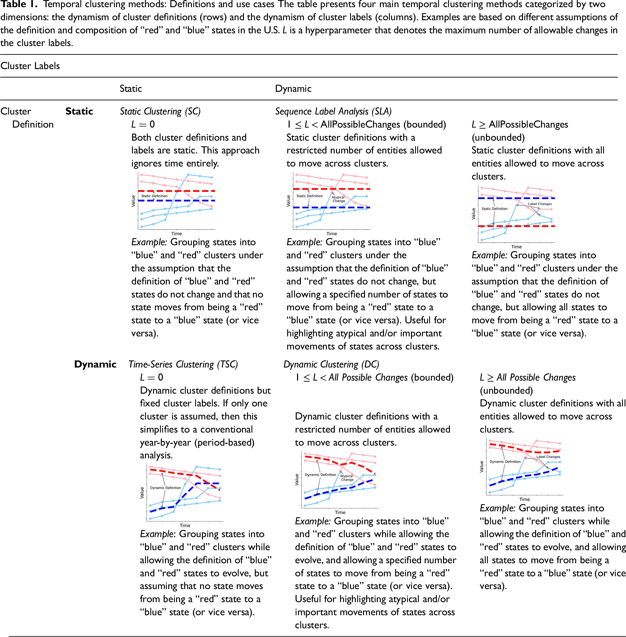
When considering different models of temporal clustering, it is important to specify the degree of dynamism of the cluster labels (i.e., how often and how many entities are allowed to transition from their original cluster assignment.) We can represent the number of allowable cluster label changes using a hyperparameter $L$ , which can range from $L = 1$ , where at most one cluster label change is allowed (illustrated in the middle part of Table 1), to $L$ equal to the total number of possible cluster label changes,⁵ where all entities are allowed to move between clusters (illustrated in the rightmost column of Table 1). We refer to temporal clustering with values of $L$ greater than the number of possible cluster label changes as unbounded and values of $L$ less than this number as bounded. Importantly, by setting lower values of $L$ , we restrict the movement of entities so that only those transitions are allowed that significantly improve the clustering objective. This is useful for highlighting more meaningful and persistent changes in the cluster labels, while filtering out more minor fluctuations. The following sections provide a detailed discussion of each temporal clustering approach and the types of changes incorporated within each method.

Cluster Definitions and Labels are Both Static

The first approach of temporal clustering assumes that the definition and composition of clusters are static. This approach, which we call Static Clustering (SC), is shown in the upper left quadrant of Table 1. With SC, the hyperparameter $L$ is zero, reflecting the assumption that there are no changes in the cluster labels. In the context of political polarization, for example, with SC the definition of a “red” and “blue” state remains constant over time. Similarly, the cluster labels are fixed, so that a state classified as “blue” will always retain that label. Because SC completely ignores temporality, both in the definition of the clusters and in the labels for each of the entities, this approach is only useful in scenarios where the primary focus is not on social change, but only on overall time-invariant clustering.

Dynamic Cluster Definitions but Static Cluster Labels

The other possibility is to assume that the cluster definitions change, but that the cluster labels are fixed, so that the composition of the clusters remains the same. This approach is shown in the lower left quadrant of Table 1 and is referred to as Time-Series Clustering or TSC for short (Aghabozorgi et al. 2015). Although uncommon in sociology and demography, TSC is a powerful method for identifying patterns and structures in evolving sequential data and has been applied in many fields, including finance, medicine, biology, and geography. TSC extends traditional center-based clustering by incorporating similarity measures that take into account entire sequences of time-ordered data. With TSC, for example, the definition of a “red” and “blue” state evolves to reflect the fact that a “red” state may increasingly be a function of mass social attitudes rather than political partisanship. However, with TSC the hyperparameter $L$ is set to zero, reflecting the assumption that no cluster labels change. Thus, like SC, a limitation of TSC is that it assumes that once an entity is in a cluster, it never leaves that cluster. In some applications this may be a highly unrealistic assumption. For example, with TSC Florida might be classified as a “blue” state for the entire duration of the observed time periods, when in reality it might be better understood as a state that moved from a “blue” cluster to a “red” cluster.

Static Cluster Definitions but Dynamic Cluster Labels

Another possibility is to assume constant cluster definitions, but allow dynamic cluster labels so that entities can move from one cluster to another. This is shown in the upper right cell of Table 1. We call this approach Sequence Label Analysis (SLA). In the context of political polarization, SLA assumes that the definition of a “red” and “blue” state does not evolve, so that any change is limited to the composition of the clusters rather than their definitions.

SLA can be understood as an adaptation of a two-step technique recently developed in studies of neighborhood evolution based on sequence analysis (Delmelle 2015, 2016, 2017; Dias and Silver 2021; Kang et al. 2020; Patias et al. 2020; Silver and Silva 2021). In the first stage, the temporal relationship is ignored by clustering each time point in each entity independently, rather than clustering the entire temporal sequence as in TSC. Each entity has an aggregated sequence constructed from the cluster labels of its time points, preserving the original temporal order. Thus, all entities are allowed to have different cluster labels at different time points. In the second step, these aggregated sequences are analyzed, for example, using similarity measures such as the optimal matching (OM) distance (Delmelle 2016; Kang et al. 2020) or Markov matrices (Silver and Silva 2021). The entire temporal data of each entity is then grouped based on the similarity between cluster label sequences or transition probabilities between clusters. The first stage of this two-stage approach is a form of SLA, as defined in Table 1.

Specifically, SLA in existing studies essentially assumes a value of $L$ that is equal to or greater than the total number of possible cluster label changes. In other words, existing SLA techniques are unbounded. This is problematic in that, by allowing all possible cluster label movements, it can be difficult to identify entities that exhibit atypical or important movements across clusters. To address this, it is often useful to set values of $L$ equal to or greater than one but less than the total number of possible cluster label changes. This results in a bounded version of SLA, such that only the top $L$ changes in cluster labels are considered valid based on their contribution to optimizing the clustering objective (i.e., by evaluating the difference in the objective with and without each potential cluster label change).⁶ By adjusting $L$ greater or equal to one but less than the total number of possible changes, bounded SLA allows one to focus on the most significant cluster label movements while filtering out less meaningful, more minor movements. The details of incorporating $L$ into the mathematical formulation of the clustering objective and the optimization process are discussed below in our discussion on the methods underlying temporal clustering.

Cluster Definitions and Labels Both Dynamic

The last logical possibility, shown in the lower right cell of Table 1, is that both the cluster definitions and the labels are dynamic. In other words, not only do the cluster definitions change, but the compositions of the clusters change as well, reflecting the fact that entities can move from one cluster to another. Temporal clustering in this category is called Dynamic Clustering (DC). In the context of political polarization, DC assumes not only that the definition of a “red” and “blue” state evolves, but so do the compositions of the clusters.

As with SLA, there are bounded and unbounded variants of DC. The unbounded version of DC corresponds to a value of $L$ that is equal to or greater than the number of possible cluster label changes. This is generally problematic, in that it can produce noisy cluster labels and definitions because it optimizes clustering independently at each time point without considering the full temporal context. In the case of fertility, this can lead to countries frequently shifting between fertility clusters due to small fluctuations rather than meaningful long-term changes in fertility rates. For example, a country with a relatively stable fertility rate close to the border of the “medium” and “high” fertility categories might oscillate between these clusters in DC year after year, obscuring the underlying stability in its fertility pattern.

For this reason, in practice the bounded version of DC is generally more desirable. This version of DC corresponds to a value of the hyperparameter $L$ that is greater than or equal to one but less than the total number of possible cluster label changes. The bounded version of DC allows one to set restrictions on the maximum number of movements across clusters. By striking a balance between flexibility and stability, the bounded version of DC is able to both capture temporal patterns among entities within each cluster as well as identify atypical temporal patterns that distinguish certain entities from the rest. This unique combination of capabilities makes DC one of the most useful and informative methods in our unified framework, providing a powerful tool for understanding complex social dynamics across time and space. The methods presented in Table 1 constitute a unified framework for analyzing how complex entities such as neighborhoods, countries, and states evolve, both in terms of cluster definitions and cluster composition. This framework yields four distinct classes of temporal clustering methods, each of which offers a unique perspective on social change by considering different combinations of static or dynamic cluster definitions and labels. While methods exist for TSC and SLA, they are not widely used in sociology and demography. Moreover, DC, which to our knowledge is an entirely new method, allows for both dynamic cluster definitions and labels, enabling the identification of complex temporal patterns and atypical trends among entities. Crucially, the hyperparameter $L$ expands the universe of possible methods, extending the capabilities of DC and SLA by setting upper limits on the number of changes in the cluster labels, thereby allowing one to strike a balance between flexibility and stability. In the next section, we discuss the optimal and scalable methods for implementing these approaches as well as other details of our methodology.

Methodology of Temporal Clustering

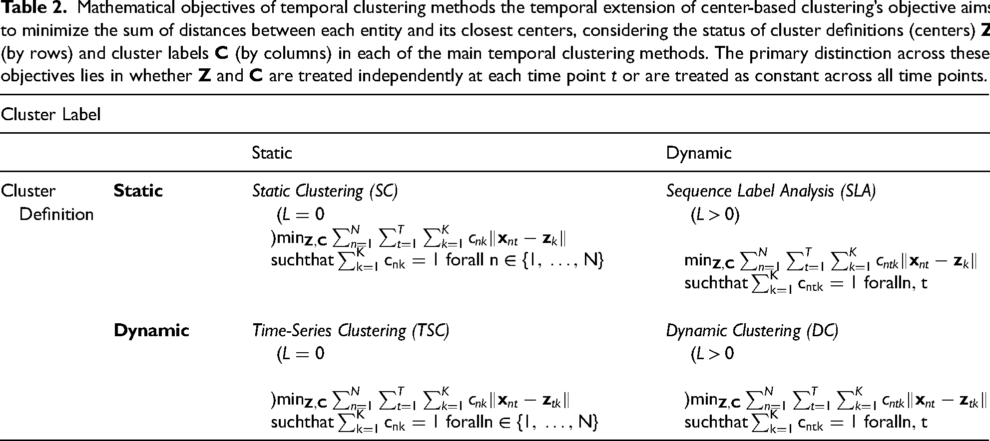
In this section, we discuss the methodology of temporal clustering, addressing the technical challenges and presenting our solutions. We formalize the criteria for optimal temporal clusters as mathematical objectives that account for intra-cluster similarity and accommodate various clustering methods, extending the objective of traditional center-based clustering to incorporate temporal relationships within the dataset. We also present the objectives for each of the four main temporal clustering methods within our unified framework in Table 2. To optimize these objectives, we briefly outline two approaches: MILP and an iterative approach inspired by the Majorize-Minimization (MM) algorithm.⁷ We conclude this section by discussing practical considerations crucial for the efficiency and interpretability of clustering results, including similarity measures, feature selection, determining the number of clusters, and setting the maximum number of cluster label changes allowed.

Table 2.

Mathematical objectives of temporal clustering methods the temporal extension of center-based clustering’s objective aims to minimize the sum of distances between each entity and its closest centers, considering the status of cluster definitions (centers) $Z$ (by rows) and cluster labels $C$ (by columns) in each of the main temporal clustering methods. The primary distinction across these objectives lies in whether $Z$ and $C$ are treated independently at each time point $t$ or are treated as constant across all time points.

Cluster Label
		Static	Dynamic
Cluster Definition	Static	Static Clustering (SC) ( $L = 0$ ) $min_{Z, C} \sum_{n = 1}^{N} \sum_{t = 1}^{T} \sum_{k = 1}^{K} c_{n k} ‖ x_{n t} - z_{k} ‖$ $such that \sum_{k = 1}^{K} c_{n k} = 1 for all n \in {1, \dots, N}$	Sequence Label Analysis (SLA) ( $L > 0$ ) $min_{Z, C} \sum_{n = 1}^{N} \sum_{t = 1}^{T} \sum_{k = 1}^{K} c_{n t k} ‖ x_{n t} - z_{k} ‖$ $such that \sum_{k = 1}^{K} c_{n t k} = 1 for all n, t$
	Dynamic	Time-Series Clustering (TSC) ( $L = 0$ ) $min_{Z, C} \sum_{n = 1}^{N} \sum_{t = 1}^{T} \sum_{k = 1}^{K} c_{n k} ‖ x_{n t} - z_{t k} ‖$ $such that \sum_{k = 1}^{K} c_{n k} = 1 for all n \in {1, \dots, N}$	Dynamic Clustering (DC) ( $L > 0$ ) $min_{Z, C} \sum_{n = 1}^{N} \sum_{t = 1}^{T} \sum_{k = 1}^{K} c_{n t k} ‖ x_{n t} - z_{t k} ‖$ $such that \sum_{k = 1}^{K} c_{n t k} = 1 for all n, t$

Clustering Objectives

Temporal clustering presents several technical challenges. First and foremost, it is crucial to rigorously define the criteria for optimal temporal clusters. We have formalized these criteria as mathematical objectives that account for intra-cluster similarity while accommodating the various clustering methods shown in Table 1. These objectives extend the traditional center-based clustering approach, which minimizes the sum of distances between each entity and its nearest center, to incorporate temporal relationships. Our objectives involve changes in both cluster labels and definitions, thereby accommodating the full range of clustering methods in our framework, from static clustering to fully dynamic approaches. Due to the technical nature of the following section, applied researchers may wish to skip to the subsequent section (“Practical Considerations”).

To clarify the discussion that follows, we introduce some notation. Let $X \in R^{N \times D \times T}$ be a temporal dataset in the real number space $R$ , where $N$ represents the total number of entities, $D$ denotes the total number of features, and $T$ signifies the total number of time points available. As well, let $K$ denote the number of clusters. We further introduce the following notation:

$x_{n t} \in X$ is a column vector with dimension $D$ denoting the values of all $D$ features at time point $t \in {1, \dots, T}$ for entity $n \in {1, \dots, N}$ .

$C$ is a binary matrix (i.e., a matrix with only entries of zero and one) with dimensions $N \times K$ representing the cluster labels of entities. Specifically, $c_{n k} \in C$ , a binary variable ${0, 1}$ , equals 1 if entity $n$ is within cluster $k \in {1, \dots, K}$ , and 0 otherwise. This can be extended to $c_{n t k} \in {0, 1}$ to account for entity $n$ at each time point $t$ separately when the temporal clustering method allows for movements of entities across clusters, as with SLA or DC.

$Z \in R^{D \times K}$ is a matrix representing the cluster centers, where $z_{k} \in Z$ is a column vector with dimension $D$ denoting the center of cluster $k$ . Analogous to $C$ , $z_{k}$ can be extended to $z_{t k}$ to represent the center of cluster $k$ at time point $t$ for clustering methods that allow the cluster centers to change over time, such as with TSC and DC.

$‖ a - b ‖$ denotes the distance measures between vector $a$ and vector $b$ using either Manhattan distance ( $l_{1}$ norm), Euclidean Distance ( $l_{2}$ norm), or any other measure as desired.

Using the notation above, Table 2 presents the mathematical objectives for each class of temporal clustering methods in our framework (cf. Table 1). As previously discussed, the primary objective of all four methods is to minimize the sum of squared distances between each entity, $x_{n} \in X$ , and its corresponding cluster center, $z_{k} \in Z$ . Specifically, the distance (e.g., Manhattan or Euclidean) between an entity $x_{n}$ and a cluster center $z_{k}$ is represented as $‖ x_{n} - z_{k} ‖$ in all four methods outlined in Table 1. Using this formulation, the sum of distances for all possible pairs between the $N$ entities and the $K$ cluster centers is given by $\sum_{n = 1}^{N} \sum_{k = 1}^{K} ‖ x_{n} - z_{k} ‖$ . However, in clustering analysis, the goal is to find the cluster assignment that minimizes this objective function. Therefore, for each entity, the distance should be considered only between the center of the cluster to which the entity is assigned, not all clusters. Thus, in each method, the distance $‖ x_{n} - z_{k} ‖$ is bounded by a binary variable, $c_{n k}$ , which indicates whether entity $n$ is assigned to cluster $k$ with center $z_{k}$ . When entity $n$ is not assigned to cluster $k$ , the distance between cluster $k$ ’s center and $n$ becomes zero, as $c_{n k} = 0$ , and does not contribute to the sum of distances. Furthermore, we assume that each entity can only be assigned to one cluster, meaning that for each entity $n$ , only one of the $c_{n k}$ values across all $k \in 1, \dots, K$ can be 1, and the rest must be 0. Hence, the second constraint in each method of Table 1 ensures that the sum of $c_{n k}$ across all $k \in 1, \dots, K$ equals 1, guaranteeing that only one $c_{n k}$ is 1. This primary objective forms the foundational structure of the clustering objective in Table 1. We must still account for variations over time points, $t \in T$ , for the purpose of temporal clustering.

The primary distinction lies in whether cluster centers $Z$ are static or dynamic, and whether or not the cluster labels $C$ are static or dynamic across time points $t \in {1, \dots, T}$ . For instance, with DC, both $z_{t k}$ and $c_{n t k}$ can vary across time point $t \in {1, \dots, T}$ within the same cluster $k$ and the same entity $n$ , accounting for its dynamic cluster centers and the fact that all possible cluster label changes may be allowed. Consequently, the clustering objective in DC should consider the “sum of distances” for the specific values of $z_{t k}$ and $c_{n t k}$ at each time point separately.

It is important to note that the clustering objectives remain unchanged for the methods in the rightmost column of Table 2, specifically SLA and DC, regardless of whether the maximum allowable label changes $L$ , is bounded or unbounded. This is because $C$ exhibits the same level of dynamism in both bounded and unbounded settings and should be evaluated independently at each time point. The key difference between these methods lies in determining the validity of the cluster label changes based on the selected $L$ value during the optimization process. Determining the appropriate value of $L$ is particularly important for methods with restrictions on the number of cluster label changes ( $1 \leq L < All Possible Changes$ ), where only the top $L$ changes are considered valid, compared to methods without such restrictions ( $L \geq All Possible Changes$ ), where all changes are assumed to be valid. Details on how to set the value of $L$ will be discussed in the following section on practical considerations when fitting temporal clustering models.

Another crucial consideration is selecting an appropriate optimization method for solving the objectives in Table 2. Traditional clustering algorithms, such as Lloyd’s algorithm for K-means clustering (Lloyd 1982), use an iterative approach inspired by the MM algorithm (Kenneth et al. 2000). We extend this method to optimize the objectives of methods for temporal clustering. The MM algorithm approximates the optimal solution by alternately updating cluster centers and reassigning entities to the updated clusters, gradually improving the clustering result until convergence. We also incorporate a post hoc analysis during each iteration to identify the top $L$ changes in cluster labels by calculating the difference in the objective with and without each possible change. The simplicity of this iterative approach allows us to obtain, in an efficient way, a near-optimal clustering result in large datasets. However, this method does not guarantee a globally optimal result and may converge to local minima (Steinley 2003), meaning it lacks reproducibility such that different initializations can lead to different local minima. To address these limitations, we also utilize MILP for optimization. MILP is guaranteed to find the globally optimal solution, ensuring reproducibility, but the trade-off is it can be computationally intensive for large datasets (Chembu et al. 2023). MILP works by formulating the clustering objectives as a series of linear equations with integer constraints, enabling joint optimization of cluster centers and labels, with the hyperparameter $L$ formalized as a constraint. Both approaches have their strengths: MILP provides optimal solutions and reproducible results for smaller datasets, while the iterative approach offers efficiency with near-optimal results for larger-scale applications. The choice between the two methods depends on the dataset size, computational resources, and the specific requirements of the research question. We refer readers to Appendix A in the online supplement for detailed discussions of these methods.

Practical Considerations

Besides selecting a suitable temporal clustering method and optimization approach for a given use case and dataset, researchers must also weigh several additional factors to maximize the effectiveness and interpretability of their results. These practical considerations can significantly influence the analysis. In this section, we outline important aspects to evaluate when implementing temporal clustering, including the choice of distance measures, feature selection and normalization, determining the optimal number of clusters, and setting restrictions on the number of cluster label changes.

Choosing a distance metric

Distance measures are widely used to assess similarity between entities and cluster centers in clustering and social sequence analysis (Aisenbrey and Anette 2010). They are effective for evaluating both feature values and temporal relationships, and are efficient for large datasets (Shieh and Keogh 2008). However, choosing the right distance measure is critical in temporal clustering, because an entity may appear close to a cluster center according to one measure, but far away according to another. Appendix B in the online supplement provides an example illustrating how different distance functions yield varying results for the same set of entities. Thus, the choice of distance measure can greatly influence the results of one’s analysis, not only for conventional clustering techniques and sequence analysis but also for temporal clustering.

Manhattan distance (also referred to as the $l_{1}$ norm) and Euclidean distance ( $l_{2}$ norm) are two distance measures commonly used in current clustering algorithms. Recall that we defined $x_{n t}$ to be the temporal data (a column vector) of an entity $n$ at time $t$ , $z_{t k}$ to be the center of cluster $k$ at time $t$ (another column vector), and $D$ as the total number of observed features in the temporal data. Then, the Manhattan distance between this entity $n$ to the center of cluster $k$ at time $t$ is defined as:

l_{1} (x_{n t}, z_{t k}) = \sum_{d = 1}^{D} | x_{n t d} - z_{t k d} | .

(1)

Likewise, the Euclidean distance is defined as

l_{2} (x_{n t}, z_{t k}) = \sqrt{\sum_{d = 1}^{D} (x_{n t d} - z_{t k d})^{2}} .

(2)

Both distance metrics share the property that if

x_{n t}

and

z_{t k}

are identical, their distance is zero. As the differences between them increase, the distance also increases indefinitely. However, they differ in their sensitivity to outliers and noise. Specifically, the Manhattan distance is less sensitive to outliers and noise in temporal data than the Euclidean distance. This is because the Euclidean distance emphasizes large differences between elements while downplaying smaller differences. It is also important to note that selecting the appropriate distance metric is challenging when clustering with multivariate features, especially when the features have different scales or units. Features with larger scales can dominate the clustering process, leading to unbalanced results. One solution to this issue is to normalize the features to ensure each contributes equally to the clustering process before clustering, which will be discussed in the next section. For readers interested in more detailed examples of how different distance functions and scales affect the measures between entities, please refer to Appendix B in the online supplement.

In general, the choice of distance measures depends highly on the temporal dataset and specific use case. We recommend starting with metric distance functions like Manhattan Distance or Euclidean Distance when applying temporal clustering. These measures are simple, effective, and scalable for large temporal datasets. In some applications, specialized similarity measures may be necessary, such as dynamic time warping (DTW) for aligning sequences with different durations or phase shifts, especially when traditional distance metrics fail to capture relevant similarities (Müller 2007). Alternatively, cosine distance, which captures the cosine of the angle between two vectors, may be useful for handling temporal sequences of different lengths after a dataset has been normalized. Regardless of the chosen measure, the selection of an appropriate distance metric is critical as it forms the basis for assessing closeness between data points, which the clustering algorithms then use to group similar entities together. For this reason, researchers should generally consider different distance measures and their impact on how the data is clustered to determine the robustness of their results.

Selecting and normalizing the features

Another important consideration is the number of features to consider when conducting a cluster analysis. An excessive number of features can increase the runtime of the optimization process as well as complicate the interpretation of temporal patterns. In general, we recommend considering features that are most relevant to the research question and that are expected to show meaningful variation across entities and time. As with any analysis, domain knowledge can guide the selection of key features.

Another related consideration is normalization. As discussed above, the distance function is sensitive to how features are scaled. Differences in feature scales can lead to distorted results, such that features with larger scales appear more substantial than those with smaller scales. Therefore, techniques such as min–max normalization and z-score normalization are essential. Normalizing each characteristic and time point separately can also eliminate common trends across entities, allowing for more interpretable comparisons between entities for certain features (e.g., mitigating the effects of inflation on median income). Because of the relative ease of implementation and interpretation, we generally recommend applying z-score normalization to each feature separately at each time point.

Determining the number of clusters

In traditional clustering, the results are sensitive to the number of clusters specified $K$ (Chiang and Mirkin 2010). This sensitivity also applies to temporal clustering. Controlling the value of $K$ can greatly improve the interpretability of the results. Kodinariya and Makwana (2013), for example, comprehensively covered several popular approaches to determining an appropriate value of $K$ . The elbow method (Yuan and Yang 2019) evaluates the reduction in the intra-cluster sum of distances as the number of clusters $K$ increases. The goal is to identify the “elbow” point where, as shown to the left of Figure 1, each successive reduction becomes relatively minimal, indicating the optimal $K$ . Intuitively, this method balances the reduction in intra-cluster variation (which always decreases as $K$ increases) with the desire for a parsimonious number of clusters. Another method, as shown to the right of Figure 1, is to find the value of $K$ that maximizes what is known as the silhouette coefficient (Rousseeuw and Kaufman 2009). This coefficient quantifies a combination of cohesion (similarity of entities within clusters) and separation (dissimilarity of entities in different clusters). A high silhouette coefficient indicates that the entities within each cluster are similar to each other, while the clusters themselves are well-separated.

Figure 1.

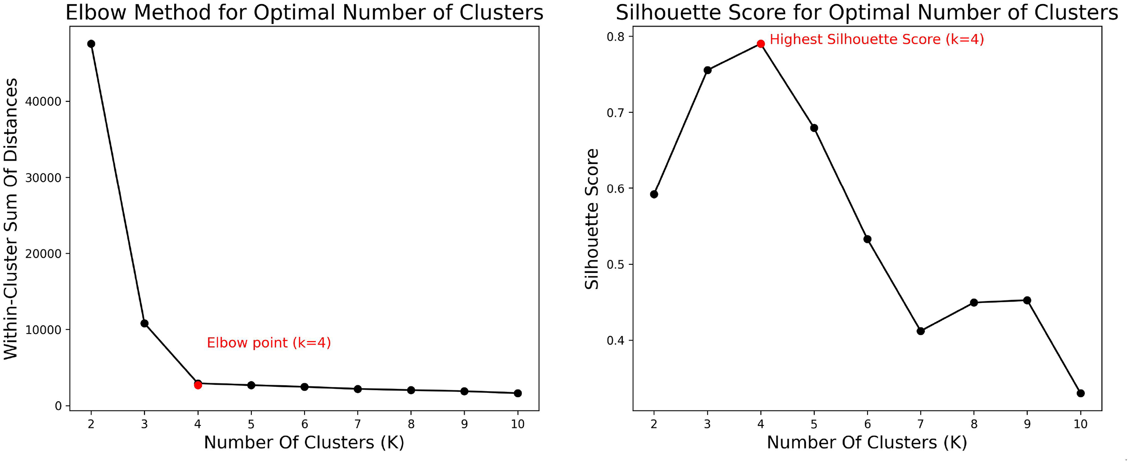
Visualization of methods for determining the optimal number of clusters $K$ . The plots below demonstrate an example of how to identify the optimal number of clusters, $K$ (indicated in red), using two methods. With the elbow method (left plot), we calculated the clustering objective, specifically the within-cluster sum of distances (y-axis), across a range of $K$ values (x-axis). The optimal $K$ was identified at that point where the decrease in the objective function transitions from steep to gradual. For the silhouette score method (right plot), the optimal $K$ was determined as the value with the highest silhouette score.

A drawback of both methods is the need to run the clustering algorithm multiple times with different values of $K$ , which may be impractical for large datasets, especially when using computationally intensive MILP formulations for optimization.⁸ Alternatively, domain knowledge can guide the selection of a few candidate $K$ values, which are then manually evaluated to determine the most suitable one for the task at hand. The optimal number of clusters should, in principle, strike a balance between capturing the salient patterns in the data while avoiding over-fragmentation of the data. We recommend using a combination of domain knowledge and data-driven methods like the elbow method or silhouette coefficient to determine the appropriate number of clusters. In practice, it is often helpful to explore a range of $K$ values and examine the interpretability and stability of the resulting clustering solutions.

Setting the maximum number of cluster label changes

The maximum number of label changes across clusters among all entities, given by the hyperparameter $L$ introduced previously, offers analytical flexibility, allowing one to consider just a few major cluster label transitions (small $L$ ) or considering more fluid movements across clusters (larger $L$ ). However, the choice of the value of $L$ can significantly impact the algorithm runtime. Increasing $L$ also increases the number of constraints in the MILP problem or the iterations required in the MM algorithm (see Figure A.1 in the online supplement). Therefore, we generally recommend starting with a small value of $L$ , such as 1 or 2, and gradually increasing it while monitoring the clustering results and runtime. The goal is to use domain knowledge in conjunction with the results obtained to identify the key transitions that significantly improve the clustering objective without including too many substantively minor shifts in the cluster labels.

Taken together, the methods presented in this section provide a comprehensive framework for temporal clustering, encompassing both mathematical foundations and practical guidelines. Researchers can effectively apply these methods by formalizing clustering objectives, exploring optimization techniques through MILP and iterative approaches, and addressing key considerations in data preparation and parameter selection to analyze complex patterns of social change. The flexibility of this framework allows for adaptation to various types of entities and temporal datasets, while also ensuring robust and interpretable results. As demonstrated in the subsequent case studies, careful application of our framework enables deeper insights into diverse sociological contexts, from political polarization to cultural value shifts to patterns of urban development.

Temporal Clustering: Sociological Examples

To evaluate and demonstrate our proposed methods, we introduce three case studies on social change: state-level social and political attitudes in the United States, cross-national cultural change in the World Values Survey (WVS), and neighborhood business development in Chicago. These cases were chosen not only because they are important topics in sociology and related fields, but also because they reveal the dynamic nature of social change, showing how entities can move between clusters as well as how new clusters emerge, reflecting evolving social, political, and cultural contexts.

The temporal clustering methods used were selected based on factors such as the number of time points and features within the dataset as well as the natural characteristics of social change of the entities (e.g., whether the definitions of clusters should evolve or remain static). In addition, we present several approaches to illustrate some of the practical considerations outlined in the previous section, in particular determining the number of clusters $K$ and setting the maximum allowable number of cluster label changes $L$ .

State-Level Temporal Polarization

The issue of political polarization in the United States has received considerable attention across a wide range of studies in various social science fields (Brown and Enos 2021; Iyengar et al. 2019). Researchers have observed that the U.S. population has increasingly shifted towards a strong affiliation with one of the two major political parties, the Democrats and the Republicans, over time. This “polarization” is evident in voting patterns, the proportion of seats in the Senate and House between the two parties in different states (Poole and Rosenthal 1984), and social attitudes as revealed in survey data. McCarty et al. (2016) also highlighted the growing disagreement on policy issues between political elites in the two parties. In our first case study, we employed temporal clustering on various cultural and political features derived from mass survey responses to evaluate prevailing accounts of population-level political polarization between states.

Existing temporal clustering methods, such as TSC and SLA, fall short as they do not account for changes in both cluster definitions and labels over time. By contrast, DC allows U.S. states to transit between Democrat-affiliated and Republican-affiliated clusters and modifies the definitions of two clusters of states. Accordingly, DC offers an arguably more realistic description of temporal polarization than existing methods, as it does not assume that a state is always Democrat-affiliated (as with TSC) or that a Democrat-affiliated cluster has an identical proportion of votes for Democrats across years (as with SLA). Furthermore, by adjusting the maximum allowable changes in labels using the hyperparameter $L$ , DC can identify a range of transitions across clusters, from the most substantial shift to relatively minor shifts. For these reasons, we selected DC as the temporal clustering method for this case study.

Dataset

Our analysis examines changes in policy views, attitudes, and partisanship across different states over the past seventy years (1946–2014). The temporal data was collected by the Correlates of State Policy Project (CSPP) (Grossmann et al. 2021), a comprehensive and publicly accessible database covering over 3,000 state policies and politics-related variables from various sources spanning seven decades. We selected five features from the CSPP for analysis. One key feature is the ratio between the proportion of Democratic and Republican identifiers in each state, indicating residents’ political affiliations. A ratio greater than one indicates a larger proportion of Democratic identifiers than Republican identifiers, while a ratio less than one suggests the opposite.⁹

We also included four CSPP measures of estimated policy and mass resident liberalism in each state. These features consist of measures of social and economic policy liberalism at the state level (“policysociallib_est” and “policyeconlib_est” in the CSPP codebook) as well as estimates of mass social and economic liberalism among state residents (“masssociallib_est” and “masseconlib_est”). The estimates of mass liberalism are constructed using public opinion surveys weighted by the proportion of identifiers in different parties (Caughey and Warshaw 2018).

Pre-proprocessing and tuning the hyperparameters

As noted above, the temporal dataset spans yearly data for the five features from 1946 to 2014 across all 50 states. For Alaska and Hawaii, which became states in 1959, data from 1949 to 1958 were imputed using the values from their first available year (1959). We observed common trends among all states in certain features, such as a general increasing trend in the mass social liberalism over the duration of the dataset. We applied z-score normalization separately per feature per year to eliminate these common trends and facilitate easier identification of notable temporal trends within entities. While we chose to apply z-score normalization in this analysis to highlight relative temporal trends within entities, we note that researchers may choose to normalize or not normalize variables based on their specific substantive goals. Importantly, the proposed framework operates seamlessly with both normalized and unnormalized inputs, without requiring any structural modifications to the clustering objectives or optimization procedures. This flexibility allows researchers to tailor the analysis to emphasize either relative patterns of change (using normalized variables) or absolute levels and shifts (using raw variables).

To determine the appropriate number of clusters $K$ , we employed a two-stage method. First, we measured the clustering objectives for different values of $K$ and selected $K = 8$ based on the diminishing reduction of the objective (the elbow method). Then, we manually evaluated each cluster definition and merged clusters with duplicate trends to avoid high similarity between different clusters. This two-step procedure resulted in specifying $K = 6$ clusters of U.S. states.

Using a similar two-stage approach, we determined the maximum allowance for changes in cluster labels as $L = 3$ . The value $L$ has a similar characteristic as the number of clusters ( $K$ ). Allowing more cluster label changes (larger $L$ ) generally reduces the clustering objective, improving the fit to the observed data, but may lead to less coherent or interpretable patterns over time, as entities switch clusters more frequently. Conversely, stricter constraints on label changes enhance the stability and substantive coherence of the clustering results, though at the potential cost of a modest increase in the clustering objective. Thus, similar to the determination of $K$ , selecting an appropriate value of $L$ involves balancing the trade-off between improving model fit and preserving meaningful temporal patterns. Researcher judgment therefore remains essential in navigating this trade-off, guided by the goals of the analysis and the nature of the substantive question.

For this particular application, we first we used the elbow method to evaluate the reduction in the DC objective as the number of allowable changes increased, similar to determining the number of clusters $K$ . While the most substantial reduction in the objective would occur with no limit on the allowable cluster label changes, this setting fails to highlight notable movements, as any changes in cluster labels are permitted. Therefore, our goal was to identify the maximum allowable changes that exhibit diminishing returns in objective reduction using the elbow method. Then, we manually evaluated the cluster label changes deemed valid to ensure there are substantively meaningful trends or shifts.¹⁰ The final, cleaned dataset consists of 69 time points, 50 entities (U.S. states), and five features, resulting in 17,250 data points. For feasibility and efficiency, we used the MM algorithm to obtain the optimized cluster definitions and labels.

Temporal clustering results

The DC method (see Figure 2) reveals a number of hidden temporal clusters and trends in the state-level temporal data.¹¹ Since all features are z-score normalized, the cluster definition for the “Ratio of Proportion of Identifiers between two Parties” feature loses its original interpretability (i.e., a value below one does not necessarily indicate a higher proportion of Republican identifiers compared to Democratic identifiers). To address this, we z-score normalized the value of one alongside other data points during pre-processing. The normalized value of one is depicted as the black dash-dot line in Figure 2. This line represents an equal proportion of identifiers between the two parties for each of the time points. Trends diverging significantly above this line suggest a stronger association with the Democratic Party, whereas values below indicate a stronger association with the Republican Party.

Figure 2.

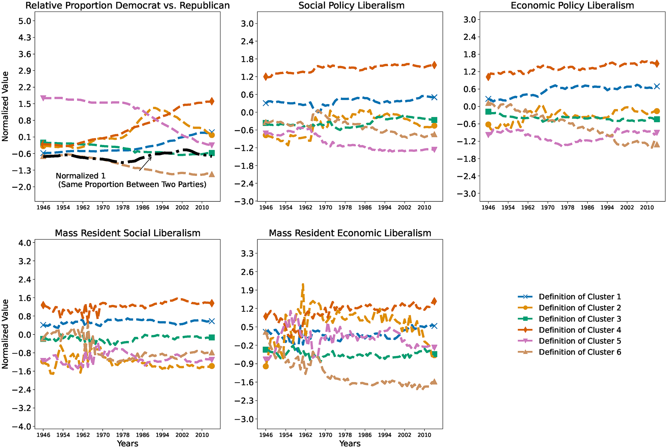
Changing definitions of “red” and “blue”: line plots of cluster definitions across U.S. States. The definition of each cluster is illustrated as dashed lines in the line plots below, with a distinct color for each cluster. Five features are used in the analysis. The black dash-dot line represents the normalized value of one, such that values above this line indicate a higher proportion of identifiers in Democratic parties and values below it indicate the opposite. For the “Relative Proportion Democrat versus Republican” feature, the temporal trends of each cluster exhibit increasing polarization over time, as illustrated by the divergence of the dashed lines from the black dash-dot line. Analyses based on DC with $K = 6$ and $L = 3$ .

Figure 2 shows increasing polarization between states, as reflected in the changing cluster definitions. This is indicated by the widening disparity in the proportions of identifiers affiliated with the two political parties over time. Initially, most clusters exhibit a nearly equal ratio between the identifiers of the two parties, suggesting a balanced distribution between parties across states. However, this ratio diverges significantly as most clusters shift towards polarized extremes. For example, the definition of cluster 1 (represented by the deep blue dashed line) increasingly aligns with the Democratic party, whereas the definitions of clusters 5 and 6 (depicted by the orange and deep red dashed lines) show a decreasing ratio, indicating a stronger association with the Republican party. These temporal trends underscore patterns of polarization in resident political orientation observed across multiple clusters of states over the years. A similar pattern is observed in the various measures of liberalism. Before 1960, there was a lack of distinction in liberalism across most clusters, such as the volatile and overlapping pattern observed in mass resident economic liberalism (see Figure 2) within cluster definitions. Post-1960, however, a significant divergence emerged in the cluster definitions, such that state policies and resident opinions on economic and social matters began to exhibit more distinct patterns across states.

Based on the geographic distribution of each cluster (illustrated in Figure 3) and a detailed analysis of the entities’ temporal data within each cluster (included in the Appendix C in the online supplement), the following sections offer an in-depth description of the six types of states. These descriptions of how clusters have changed with respect to political affiliation, liberalism in economic and social policies, and residents’ opinions on economic and social issues.

Figure 3.

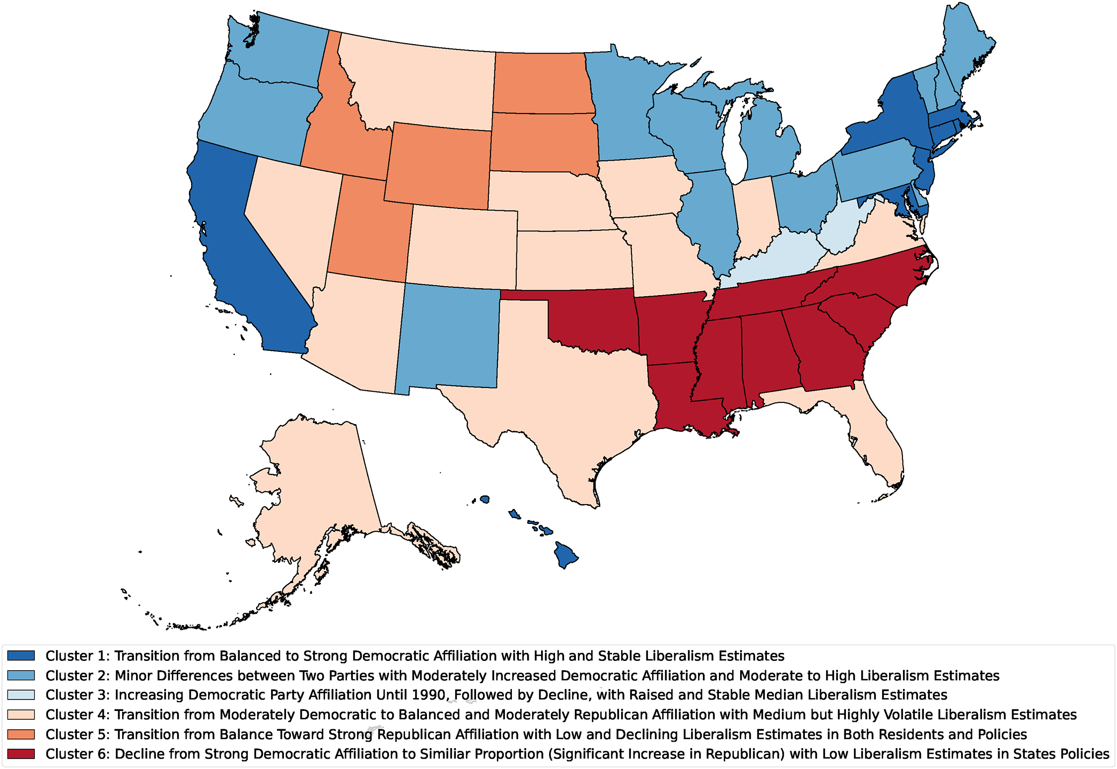
Geographical distribution of sociopolitical clusters in 2014. This choropleth map depicts the distribution of U.S. states across six clusters in the final year of observation, 2014, based on five features related to political affiliation, mass liberalism, and policy liberalism. The legend provides a brief description of each cluster’s temporal pattern. Notably, Texas was initially part of Cluster 6 but shifted to Cluster 4 in 1984. Alaska and Oklahoma also experienced shifts in their cluster labels: Alaska moved from Cluster 2 to Cluster 4 in 2000, and Oklahoma transitioned from Cluster 4 to Cluster 6 in 1983. The geographical distribution of clusters before any changes in cluster labels, as determined by DC’s results, is shown in Figure 4. Analyses based on DC with $K = 6$ and $L = 3$ .

Cluster 1: Transition from balanced to strong democratic affiliation with high and stable liberalism

The states in Cluster 1 initially had a similar proportion of identifiers between the two parties, indicated by a ratio near one before 1960. Subsequently, the ratio shifted significantly toward the Democratic party, with a pronounced increasing trend, making this cluster the highest average ratio among all states after 2000. This trend suggests a continuously increasing and strong affiliation toward the Democratic party among the residents of these states.The four types of liberalism measures in these states consistently ranked among the highest of all states throughout the studied period. Resident economic liberalism increased from the 75th percentile to the highest rank between 1946 and 1960. This temporal pattern reveals a high degree of liberalism in both states’ policies and residents’ opinions.¹²

Cluster 2: Minor differences between two parties with moderately increased democratic affiliation and moderate to high liberalism

The time series of the five features for the states within Cluster 2 maintained a small difference in the proportion of residents identifying with the Democratic and Republican parties, with a slightly higher proportion of Democratic identifiers. This stable ratio indicates a persistent partisan lean favoring the Democratic party over the Republican party.

The temporal trends of estimated liberalism for both policies and residents exhibit distinct patterns in two epochs, before and after 1970. Before 1970 there was higher volatility in all four measures of liberalism, particularly in mass resident economic liberalism, which fluctuated between high and low levels without clear trends shared among states.¹³ After 1970, volatility decreased significantly within all four types of liberalism, indicating more stable state-level policies and residents’ social and economic attitudes. Cluster 2’s temporal pattern stabilized around the 75th percentile among all states, revealing a moderate and high degree of liberalism in states within this cluster after 1970.

Cluster 3: Increasing democratic party affiliation until 1990, followed by decline, with high and stable median liberalism

Cluster 3 includes only two states, West Virginia and Kentucky, but demonstrates distinct temporal trends in the features, making it a unique cluster. The ratio between the proportions of identifiers in the two political parties exhibits three stages over the years. First, before 1960 the ratio maintained a consistent value, indicating a stronger affiliation with the Democratic Party, though the difference was relatively insignificant. Next, from 1960 to 1990, there was a significant increase in the ratio, indicating a larger proportion of residents affiliating with the Democratic Party. Finally, from 1990 to 2012, this high ratio toward the Democratic Party declined, shifting back to a range similar to that before 1960. Note, however, that the Democratic Party has maintained a substantial proportion of residents in these two states.

The measures of liberalism also reflect similar temporal stages as the party affiliation ratio. Before 1960, the estimated liberalism of economic-related policies and resident opinion on economic matters exhibited upward trends from the 25th percentile to the median among all states, while the two measures of social liberalism remained within the 25th percentile. Then, from 1960 to 2000, social policy first showed an increasing trend into the median and maintained within the median rank alongside economic policy liberalism. Mass resident liberalism exhibited two polarized trends: while resident economic liberalism continued to rise into the 75th percentile from the median, resident social liberalism remained within the lowest range of all states. After 2000, there was a significant declining trend in resident economic liberalism back toward the median to the 25th percentile, revealing low liberalism in mass resident opinions on economic and social matters, while the two types of policy liberalism maintained the median rank.

Cluster 4: Transition from moderately democratic to balanced and moderately republican affiliation with medium but highly volatile liberalism

In terms of partisanship, Cluster 4 indicated a tendency toward Democratic affiliation before 1960, as evidenced by the ratio of identifiers greater than one. After 1960, this ratio decreased, suggesting an increasing proportion of Republican identifiers, and after 1990 both parties had a similar proportion of identifiers in these states, with some states having a higher proportion of Republican identifiers. This trend continued through 2014, the last year in our data.

Measures of liberalism in some states within this cluster show high volatility. For example, Colorado experienced a significant drop from a high ranking in economic policy liberalism to the 25th percentile. Nevertheless, the cluster definition, which represents the average of all states in this cluster, shows relatively stable trends. This stability can be attributed to two factors. First, most states with high volatility shifted within a small range of values. Second, states with high volatility in trends make up a small proportion of this cluster. The cluster definition shows that social liberalism in state policies and residents’ opinions has remained within the median of all states. By contrast, economic liberalism in these states is in a lower range, between the median and the 25th percentile.

Cluster 5: Transition from balance toward strong republican affiliation with low and declining liberalism estimates in both residents and policies

The states in Cluster 5 show an increasing tendency to become more Republican over time. This shift is evident in the two-step transition of the ratio of party identifiers. Prior to 1975, both parties had comparable proportions of identifiers among residents, resulting in a ratio of nearly one to one. After 1975, however, this ratio declined significantly, falling below one, indicating that the proportion of Republican identifiers exceeded that of Democratic identifiers in these states. Along with this shift in partisanship, measures of economic liberalism among both residents and state policies show a significant downward trend. These measures of economic liberalism initially ranged between the median and 75th percentile, but eventually fell to around the 25th percentile or lower, suggesting that economic policies and opinions in these states are becoming less liberal. A similar, though less pronounced, downward trend is observed for both policies and attitudes on social issues.

Cluster 6: Decline from strong democratic affiliation to similar proportion (Significant increase in republican) with low liberalism estimates in state policies

States in Cluster 6 had the highest ratio of two-party identifiers before 1960, with some states showing increasing Democratic Party affiliation, indicating a strong Democratic alignment among residents. However, this pattern shifted after 1960, with most states in the cluster experiencing a declining trend in this ratio. The timing of this decline varied; for example, Alabama maintained its increasing trend toward the Democratic Party until 1976, while Louisiana’s decline began in 1964. This temporal trend reveals a substantial increase in the proportion of Republican identifiers and a corresponding decrease in Democratic identifiers, transforming these states from strongly Democratic to more Republican-leaning.

Measures of liberalism in states’ social policies, economic policies, and residents’ opinions on social issues consistently remained between the lowest rank and the 25th percentile, suggesting relatively low liberalism in state policies on economic and social issues, along with a declining trend in mass social liberalism. By contrast, residents’ opinions on economic issues underwent a two-stage evolution. Before 1960, it showed an increasing trend from the 25th percentile to between the 75th and the highest ranks, indicating a relatively high degree of economic liberalism among residents. After 1960, it declined and stabilized around the median, showing a decline in economic liberalism but still at a higher level than the other measures of liberalism in this cluster.

Before turning to our analysis of notable movements across clusters, it is important to clarify the relationship between continuous measurement and categorical clustering in our approach. Although we occasionally invoke familiar political terms such as “blue” and “red” states to aid interpretation, these labels were not produced by our clustering methods. Rather than imposing binary thresholds (e.g., strict Democratic or Republican cutoffs), our framework identifies six distinct clusters based on shared trajectories within a continuous, multidimensional feature space. The underlying cluster definitions remain fully embedded in continuous variables over time in Figure 2. The number of clusters ( $K$ ) is also customizable, allowing researchers to adjust the granularity of the analysis depending on the substantive goals. While clustering inherently entails a degree of information compression, this is essential for uncovering structured insights from complex longitudinal data. In this way, our framework avoids arbitrary categorical simplifications and instead highlights meaningful dynamics between entities across time.

Analysis of notable movements of states across clusters

Using values of $L$ less than the total number of possible changes in cluster labels, the bound version of DC can be used to highlight notable or atypical movements of states across the clusters described above. By setting $L = 3$ , the DC method has identified the transitions in these three states as the three most notable among all possible year-to-year shifts in the data. Figure 4 shows the geographic distribution of clusters based on each state’s cluster label in 1982, before any transitions between clusters. This contrasts with the geographic distribution in 2014 (Figure 3), where three states now have different cluster labels: Oklahoma (Cluster 4 in 1982, Cluster 6 in 2014), Texas (Cluster 6 in 1982, Cluster 4 in 2014), and Alaska (Cluster 2 in 1982, Cluster 4 in 2014). Figure 5 shows the time series of these three states for each of the five features.

Figure 4.

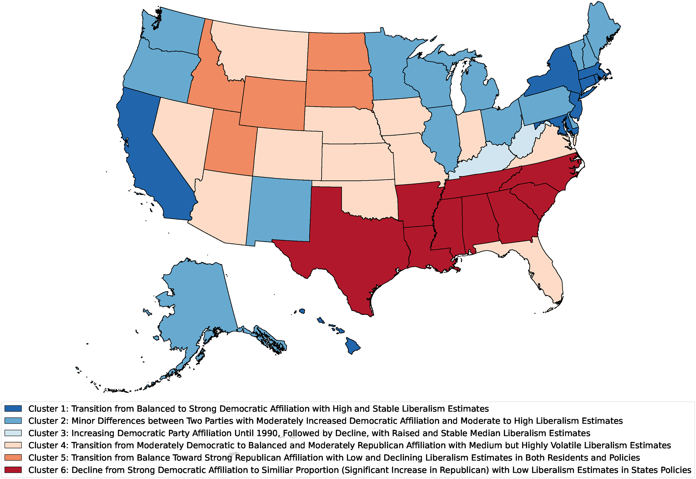
Geographical distribution of sociopolitical clusters in 1982. This choropleth map illustrates the distribution of states across six clusters in 1982 using the same five features. As mentioned in Figure 3, Texas, Alaska, and Oklahoma were in a different cluster in 1982 than their final cluster label, indicating notable changes in their cluster labels. Analyses based on DC with $K = 6$ and $L = 3$

Figure 5.

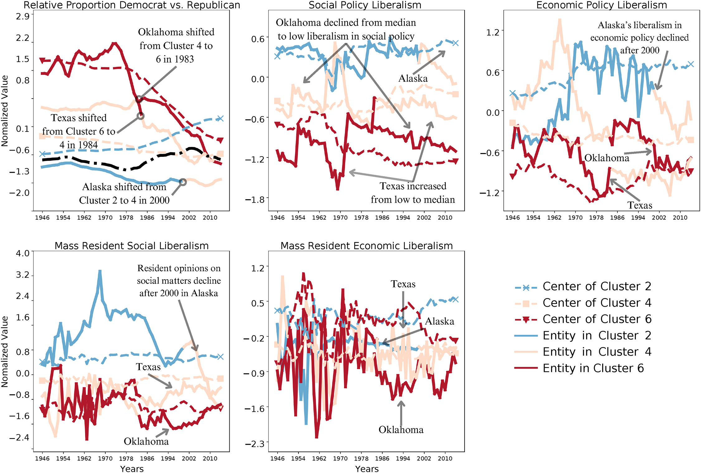
Line plots of features for the U.S. states with notable movements across clusters. The time series features of the three states (illustrated with a solid line with text annotation on the side) that exhibited changes in their cluster labels (illustrated as changes in the color of the line segment within a single state). Dashed lines indicate the definitions of the clusters. Analyses based on DC with $K = 6$ and $L = 3$ .

In 1983, Oklahoma moved from Cluster 4 to Cluster 6. Oklahoma’s time series in the relative proportion of Democrats (vs. Republicans) shows that prior to the transition to Cluster 4 in 1983, it had a stable trend with a higher proportion of Democratic identifiers, which closely matches the definition of Cluster 4 (pink dashed line in Figure 5). However, the slope of its declining trend differs from the Cluster 4 definition and the other states in Cluster 4. This slope indicates a substantial shift in Oklahoma, more in line with the temporal pattern of Cluster 6 (red dashed line). If Oklahoma were statically assigned to Cluster 6 such that time were ignored, its trend before 1983 would show little similarity to the definition of Cluster 6, as Oklahoma has a significantly smaller share of Democrats compared to the other states in Cluster 6.

Further analysis revealed similar characteristics in other features contributing to this change. For example, Cluster 4 has maintained median ranges in estimated liberalism and state policies over the years (pink dashed line in the social and economic policy measures in Figure 5). By contrast, the states in Cluster 6 (red dashed line) show a continuous decline, with lower scores on these liberalism measures than in Cluster 4. Prior to 1983, Oklahoma showed stable liberalism with median values that fit only with Cluster 4. Conversely, Oklahoma’s declining trend after 1983 fits only with Cluster 6, indicating that Oklahoma embodies two different temporal patterns, marking it as a state with a notable shift in its cluster label.¹⁴

Similar scenarios are evident in two other states that experienced changes in their cluster labels. For example, Alaska moved from Cluster 2 to Cluster 4 in 2000 due to a decline in the liberalism of social and economic policies as well as in residents’ opinions on social issues. This decline distinguishes it from the other states in Cluster 4, which maintain measures of liberalism at the 75th percentile throughout the years studied. In addition, Alaska lacks the increasing trend in the proportion of Democratic versus Republican identifiers that is evident in the definition of Cluster 2 (blue dashed line in Figure 5). These unique patterns observed in Alaska led to a change in its cluster label in 2000 to Cluster 4, which has a more similar temporal pattern to Alaska after 2000.

Texas shifted from Cluster 6 to Cluster 4 because of an increase in the liberalism of social policies and residents’ opinions on social issues between 1970 and 1980. The trend thereafter sets Texas apart from the low and declining pattern of Cluster 6 and aligns it more with the stable trend within the median range in Cluster 4. Texas also had an earlier and faster decline in the proportion of identifiers from the two major political parties around 1970 than other states in Cluster 6. After 2000, unlike the temporal pattern observed in the Cluster 6 definition, which shows a continuous declining trend through the end of the years studied, Texas maintained a stable and balanced proportion between the two parties. Consequently, all of the observed differences in Texas support an earlier transition from a state with a high Democratic affiliation to one with a balance between the two political parties compared to other states with similar temporal patterns. Furthermore, Texas exhibits a higher degree of social liberalism, both in its policies and among its residents. These unique temporal patterns are reflected in a change in its cluster label in 1984, as shown in Figure 5.

This case study underscores the power of DC to reveal complex patterns of social change. In describing the dynamic nature of polarization in the United States, DC accounts for both the fluidity of state affiliations as well as the evolving meaning of “red” and “blue” clusters. Our analysis has highlighted six distinct clusters as well as three states, Oklahoma, Texas, and Alaska, that deviate from the broader shifts in cluster definitions, moving from one cluster to another.

Global Cultural Change: World Values Survey

For our second case study, we investigate cross-national changes in cultural values using the WVS (Haerpfer et al. 2022). First, we provide empirical definitions of four types of countries based on ten indicators across three time points aggregated from seven waves of the WVS conducted from 1981 to 2022. We then analyze how countries transition between these types over time to examine cultural changes.

Overview

The WVS is an ongoing research program that aims to measure the cultural values and beliefs of citizens in different countries using standardized questionnaires. A notable research product of the WVS is the “Inglehart–Welzel Cultural Map” (Inglehart 2006), which categorizes countries in each survey wave into distinct cultural clusters. The core methodology involves subsetting to each wave of the WVS, applying factor analysis to select ten indicators, and clustering countries based on their positions in the resulting two-dimensional space. The dimensions represent “Traditional” versus “Secular-Rational’ values and “Survival” versus “Self-expression” values (Inglehart 2006). Next, the countries are grouped manually into nine cultural zones (cf. Huntington 2020) taking into account factors such as language, geography, and religion. Patterns of social change are then identified by visually examining shifts in this two-dimensional space across survey waves.

Despite the immense contributions of the work by Inglehart and colleagues to ongoing debates about the nature and extent of cultural change around the world, their main clustering approach has several limitations. First, reducing the original ten features to just two dimensions through factor analysis can lead to a considerable loss of information. Second, the manual clustering approach lacks a clear mathematical objective, rendering the results subjective and challenging to reproduce. Additionally, since the analysis is performed independently for each wave of survey responses with different subsets of countries, there is a risk of inconsistency in the definition of reduced dimensional space across years. Finally, the cultural zone definitions are based on external, ad hoc decisions that can significantly affect the conclusions drawn from the analysis. As we show below, our proposed temporal clustering framework can address these issues and provide a more rigorous, data-driven analysis of global cultural change using the WVS data.

Dataset

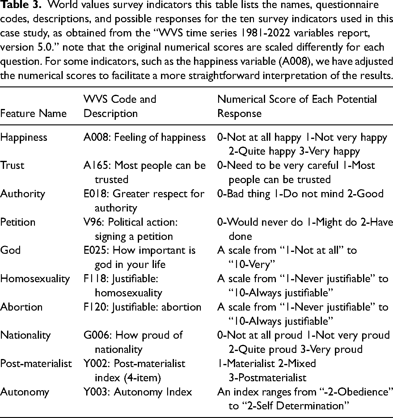
We aggregated the seven WVS waves from 1981 to 2022 into three time points to maximize the number of countries with complete data for the ten selected indicators (see Table 3). The scores of the features were calculated as the mean of the survey responses per country, taking into account sampling weights and eliminating missing responses. Z-Score normalization was applied to each feature to ensure all features are under the same scale. The resulting dataset covers 30 countries across three time points, with ten features capturing various aspects of cultural change.

Table 3.

World values survey indicators this table lists the names, questionnaire codes, descriptions, and possible responses for the ten survey indicators used in this case study, as obtained from the “WVS time series 1981-2022 variables report, version 5.0.” note that the original numerical scores are scaled differently for each question. For some indicators, such as the happiness variable (A008), we have adjusted the numerical scores to facilitate a more straightforward interpretation of the results.

Feature Name	WVS Code and Description	Numerical Score of Each Potential Response
Happiness	A008: Feeling of happiness	0-Not at all happy 1-Not very happy 2-Quite happy 3-Very happy
Trust	A165: Most people can be trusted	0-Need to be very careful 1-Most people can be trusted
Authority	E018: Greater respect for authority	0-Bad thing 1-Do not mind 2-Good
Petition	V96: Political action: signing a petition	0-Would never do 1-Might do 2-Have done
God	E025: How important is god in your life	A scale from “1-Not at all” to “10-Very”
Homosexuality	F118: Justifiable: homosexuality	A scale from “1-Never justifiable” to “10-Always justifiable”
Abortion	F120: Justifiable: abortion	A scale from “1-Never justifiable” to “10-Always justifiable”
Nationality	G006: How proud of nationality	0-Not at all proud 1-Not very proud 2-Quite proud 3-Very proud
Post-materialist	Y002: Post-materialist index (4-item)	1-Materialist 2-Mixed 3-Postmaterialist
Autonomy	Y003: Autonomy Index	An index ranges from “-2-Obedience” to “2-Self Determination”

Methods and hyperparameters

Recall that SLA assumes that the cluster definitions remain constant over time, making it most suitable for datasets with few time points.¹⁵ Moreover, when dealing with high-dimensional datasets containing many features, SLA can provide easily interpretable results. Moreover, as we show below, by using the bounded version of SLA, where we set the maximum number of allowed cluster label changes ( $L$ ) greater than zero but less than the total number of possible changes, we can limit the number of times countries transition between clusters, helping us identify the most important and atypical transitions. Given the relatively small size of the dataset, MILP optimization is feasible, ensuring that the solution is globally optimal and reproducible. In this example, we set the number of clusters ( $K$ ) to 4 to maintain general consistency with the original work by Inglehart and colleagues.

Detailed cluster definitions

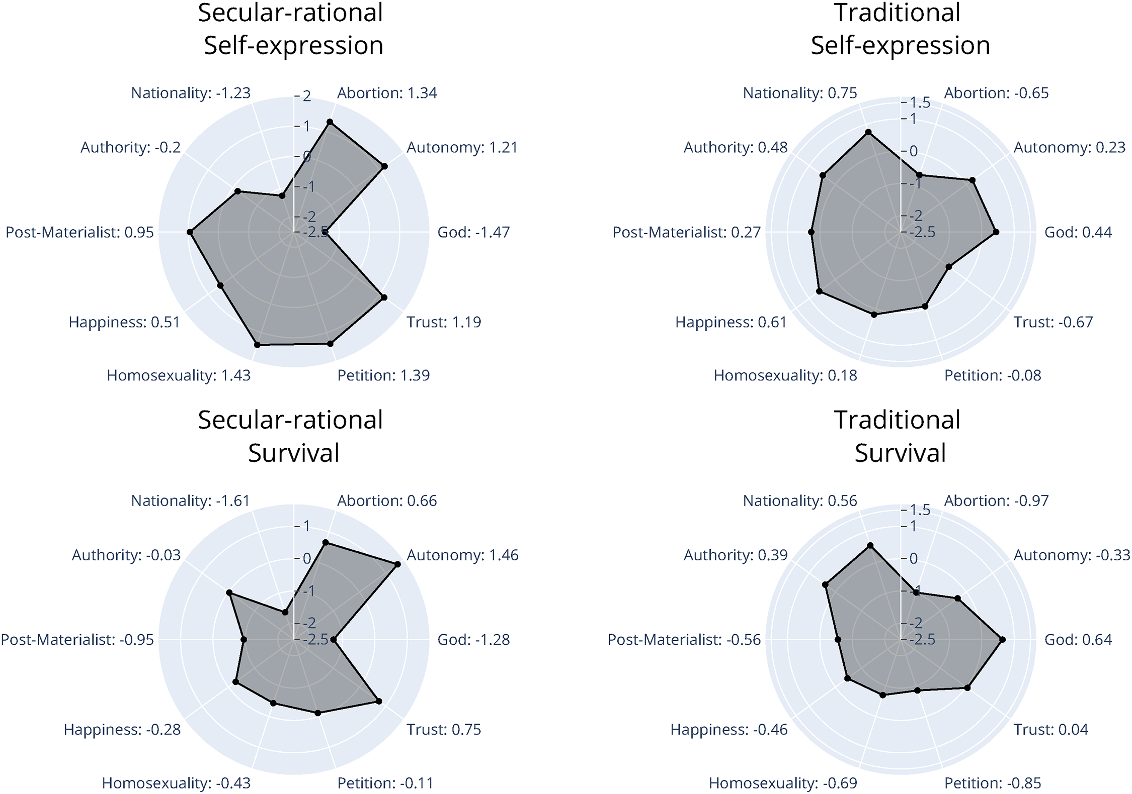
To begin our analysis, we applied the unbounded version of SLA, where $L$ is set to allow all possible cluster label changes. Accordingly, all countries are allowed to move freely across clusters over time, while the cluster definitions remain constant.¹⁶ To help us interpret the cluster definitions, we created radar plots for each cluster that shows the relationships between the ten survey indicators and the center of each cluster (see Figure 6). It is important to note that, in contrast to the approach used by Inglehart (2006), these definitions are based directly on the average survey responses rather than extracted principal components.

Figure 6.

Cluster definitions in the world values surveys. The radar plots depict the cluster definitions as the scores on the ten survey indicators used. Analyses based on SLA with $K = 4$ and $L$ set to the maximum number of allowed cluster label changes.

Cluster 1 (Secular-Rational and Self-expression Values): Unlike the societies in the traditional-survival values cluster, these countries display strong secular-rational and self-expression values, as shown in the upper left radar plot in Figure 6. They are characterized by a higher acceptance of abortion, less importance placed on religion, lower national pride, less respect for authority, and a greater emphasis on autonomy. Additionally, these countries report high levels of happiness, greater justification for homosexuality, and higher trust in others.

Cluster 2 (Traditional and Self-Expression Values): This cluster, shown in the upper right radar plot of Figure 6, consists of countries that combine traditional with self-expression values. These countries place a higher importance on God, have the highest respect for authority, and exhibit the highest national pride. Interestingly, they also report the highest happiness levels, post-materialist tendencies, and a higher acceptance of homosexuality, which are indicative of self-expression values. However, there are some contradictory patterns, such as lower trust in others.

Cluster 3 (Secular-Rational and Survival Values): This cluster is visualized in the lower left radar plot of Figure 6, and consists of countries with high secular and rational values, such as a lower importance of religion, lower national pride, and more self-determination, with survival values, including the highest levels of unhappiness, materialism, and low justification for homosexuality. Note, however, countries in this cluster also exhibit some levels on some items that align with self-expression values, such as a greater trust in others.

Cluster 4 (Traditional and Survival Values): Finally, this cluster consists of countries that exhibit both high levels of traditional and survival values, as shown in the lower right radar plot in Figure 6. These countries place a high importance on God, show the lowest justification for abortion, have strong national pride, and respect authorities. They also report low levels of happiness, minimal justification for homosexuality, a reluctance to sign petitions, and a general distrust of others.

Note that SLA directly incorporates the average survey responses into the cluster definitions, providing specific scores for each indicator. This contrasts with the manual clustering and reduction to two principal components used in the original “Inglehart–Welzel Cultural Map.” However, to compare our results to those from Inglehart and colleagues (2006), it is informative to visualize the distributions of the countries within each cluster across the first two principal components derived from the ten survey items.

In Figure 7, we show the position of each country at each of the three aggregated time points, along with the centers of the four clusters. Cluster labels for each time point are represented by different colors, with the center of each cluster indicated by crosses. The colored regions are formed by connecting four archetypal points (Stone and Cutler 1996) of entities within each cluster. Similar to Inglehart (2006), the first two principal components in Figure 7 reveal two key dimensions of cross-cultural variation: (a) traditional versus secular-rational values and (b) survival versus self-expression values. For instance, a lower score on the first principal component (y-axis) indicates that a country leans more towards traditional values, while a higher score indicates a stronger alignment with secular-rational values. The centers of the four clusters, represented by colored crosses, are positioned at the extremes of these dimensions, defining four distinct value types.

Figure 7.

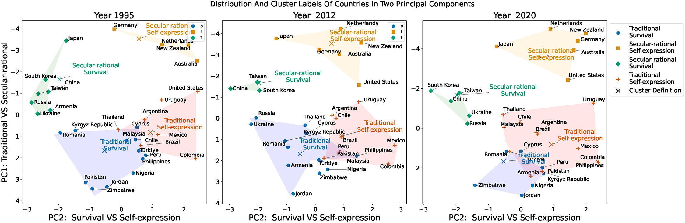
Cultural maps of 30 countries across three time points. To compare our results with those from Inglehart and colleagues (2006), the distribution of each country at each aggregated time point is plotted using the first two principal components derived from ten survey indicators. Cluster labels for each time point are represented by different colors, with the center of each cluster indicated by crosses. The colored regions are formed by connecting four archetypal points of entities within each cluster. Analyses based on SLA with $K = 4$ and $L$ set to the maximum number of allowed cluster label changes.

Figure 7 shows, with remarkable detail, how countries have evolved with respect to Inglehart’s fundamental value orientations. To better understand this figure, recall that SLA assumes the cluster definitions remain the same over time (see Table 1). Accordingly, in Figure 7, the position of cluster centers (represented by colored crosses) are fixed across all three time points. However, in contrast to the fixed cluster centers, SLA allows for dynamic cluster labels, meaning that countries can shift between clusters as their positions on the plot change, moving closer to the center of a different cluster at different time points. These transitions are illustrated by the fact that a single country’s label can appear in different colors across the three plots in Figure 7. For instance, in 1995 and 2012, the United States was grouped into Cluster 2 (Traditional and Self-Expression Values), as it was located closest to the center of this cluster (marked by a red cross). However, as the United States’ position shifted toward secular-rational values, it became closer to the center of Cluster 1 (Secular-Rational and Self-expression Values), thereby resulting in a change in its cluster label.

A similar situation occurred with Russia and Ukraine. In 1995, these countries were part of Cluster 3 (Secular-Rational and Survival Values). However, they moved from secular-rational to traditional values in 2012, causing a shift in their labels to Cluster 4 (Traditional and Survival Values). Then, in 2020, Russia and Ukraine shifted back to Cluster 3 (Secular-Rational and Survival Values). It is important to note that, compared to the United States, the positional shifts of Russia and Ukraine were less notable in Figure 7. When entities can move between clusters without restriction (i.e., $L \geq All Possible Changes$ ), it becomes challenging to identify the most meaningful and/or atypical transitions among countries. This is because all changes in cluster labels are considered valid, making it difficult to distinguish minor fluctuations from major shifts in cultural values. To address this limitation, we can adjust the maximum number of allowable label changes, $L$ , to a value greater than zero but less than the total number of possible changes (i.e., $1 \leq L < All Possible Changes$ ). By setting a lower value of $L$ , we restrict the movement of entities so that only those transitions that significantly improve the clustering objective are allowed. This bounded version of SLA helps to highlight more meaningful and persistent changes in the cluster labels while filtering out minor fluctuations. In the next section, we illustrate how this bounded version of SLA can highlight important shifts in cluster labels.

Identifying notable movements between clusters

The results so far are based on the unbounded version of SLA, where $L$ is equal to or greater than the total number of possible changes (e.g., see Figure 7). However, as noted above, one limitation of this approach is that it can be difficult to determine which cluster label changes are the most important. Accordingly, to identify some of the key atypical cluster label changes across clusters, we set the maximum number of allowed cluster label changes to $L = 3$ . This retains the cluster definitions we outlined earlier, but also the top three atypical cluster label changes (see Figure C.1 in Appendix C of the online supplement), prioritizing those that most significantly reduce the clustering objective: Pakistan, Japan, and the United States. It is important to underscore that these countries were selected based on the SLA method, and not in ad hoc way.

Pakistan: From survival to self-expression

Pakistan experienced a notable shift from Cluster 4 (Traditional and Survival Values) to Cluster 2 (Traditional and Self-expression Values), reflecting a fundamental shift change from survival to self-expression values. As shown in Figure 8, Pakistan shifted towards higher levels of happiness, as well as a shift from materialist to post-materialist values, both of which are consistent with a transition from Cluster 4 to Cluster 2.

Figure 8.

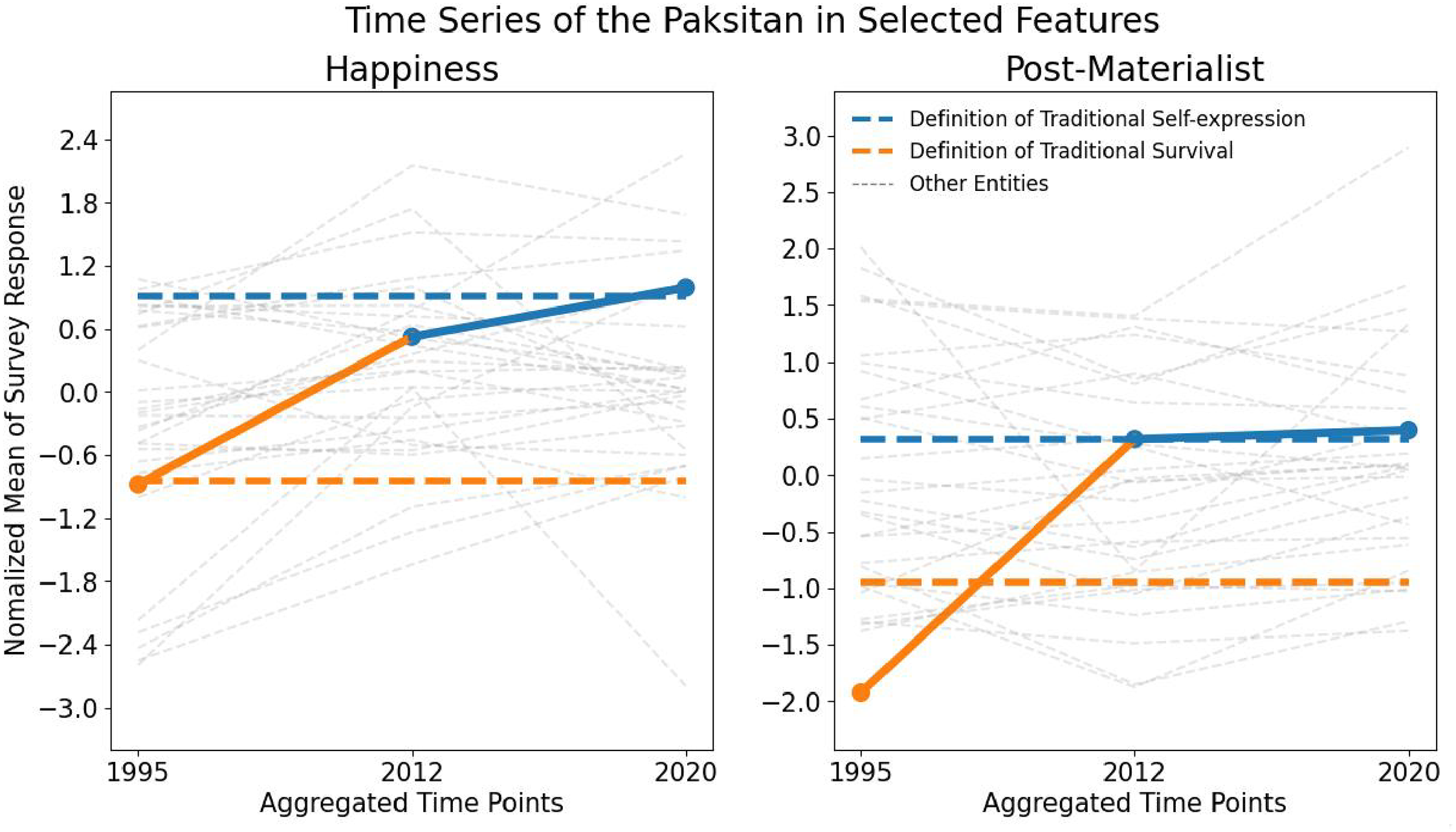
Pakistan: temporal changes on selected indicators. These line plots depict the mean survey responses for happiness and post-materialist values in Pakistan across three aggregated time points. The color-coded line segments indicate the cluster labels at each time point, while the dashed lines denote the cluster definitions, which are static. These results are consistent with the Pakistan’s movement from Cluster 4 to Cluster 2, reflecting a shift from survival to self-expression values. Analyses are based on SLA with $K = 4$ and $L = 3$ .

Japan: From survival to self-expression

Japan shifted from Cluster 3 (Secular-Rational and Survival Values) to Cluster 1 (Secular-Rational and Self-Expression Values). Japan is notable in that it exhibited a substantial increase in the belief that homosexuality is justified (see Figure 9), setting it apart from other East Asian countries. Alongside this trend was a shift towards higher levels of happiness, such that country became increasingly aligned with the center of Cluster 1 rather than Cluster 3. Note that Japan’s transition from survival to self-expression values is consistent with the trends presented by Inglehart (2006).

Figure 9.

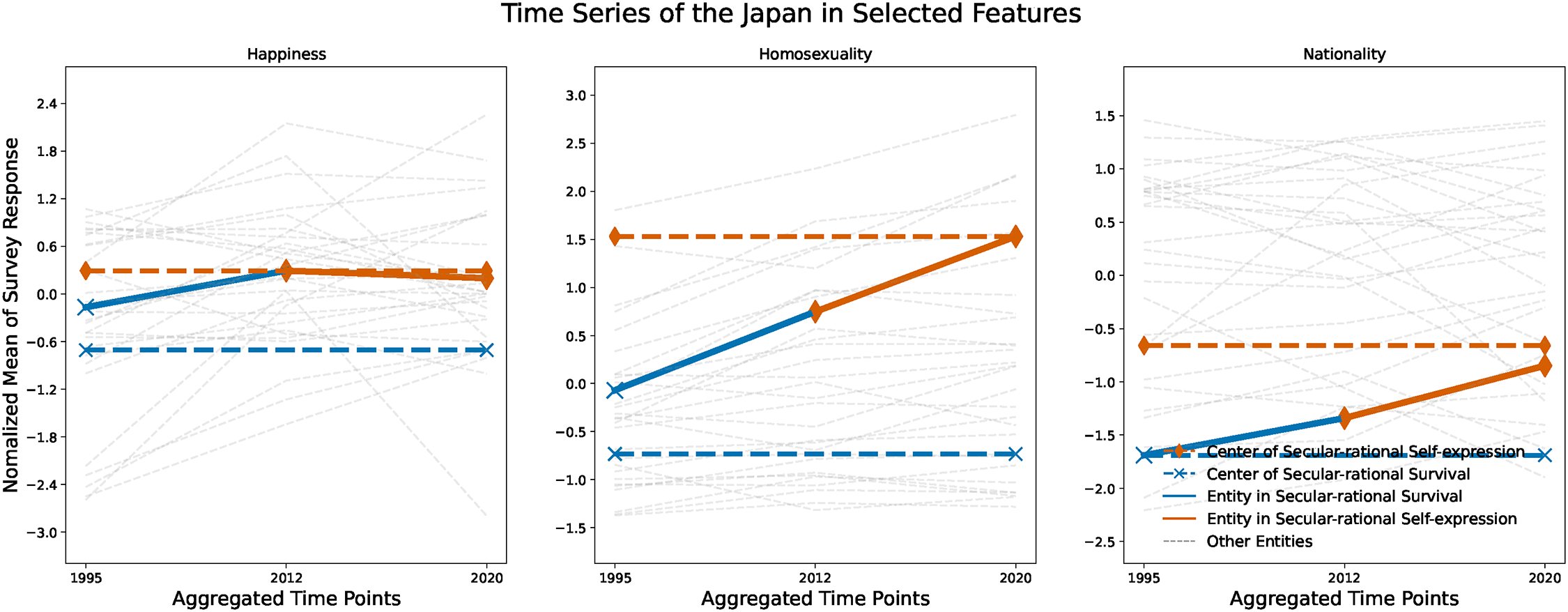
Japan: temporal changes on selected indicators. These lines plots depict the mean survey responses for happiness, views on homosexuality, and pride in nationality in Japan across three time points. The color-coded line segments indicate the cluster labels at each time point, while the dashed lines denote the cluster definitions, which are static. These results are consistent with the Japan’s movement from Cluster 3 to Cluster 1, reflecting a shift from survival to self-expression values. Analyses are based on SLA with $K = 4$ and $L = 3$ .

United States: From traditional to secular-rational

The United States shifted from Cluster 2 (Traditional and Self-Expression Values) to Cluster 1 (Secular-Rational and Self-Expression Values), reflecting an underlying shift from traditional to secular-rational values. As shown in Figure 10, the data indicates a decrease in national pride, less respect for authority, and a decline in the importance of God, all of which are consistent with this shift in values.

Figure 10.

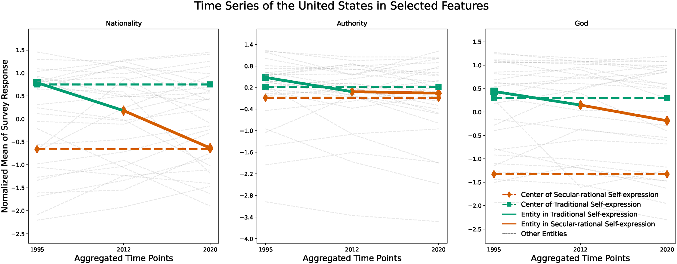
United States: temporal changes in selected indicators. These line plots illustrate the three selected features across three time points based on the mean survey responses in the United States. The color-coded line segments indicate the cluster labels at each time point, while the dashed lines denote the cluster definitions, which are static. These results are consistent with the United States’ movement from Cluster 2 to Cluster 1, reflecting a shift from traditional to secular-rational values. Analyses are based on SLA with $K = 4$ and $L = 3$ .

This case study demonstrates the utility of our temporal clustering framework for analyzing global cultural change using the WVS data. By applying SLA, we obtained detailed definitions of four cultural clusters and directly showed how these clusters relate to the ten major survey items commonly used to examine cross-national cultural change in the WVS. In addition, we illustrate a method for identifying important shifts in cluster labels by setting the value of the hyperparameter $L$ to a relatively small value, resulting in a bounded version of the SLA. As we show, Pakistan, Japan, and the United States in particular have experienced major cultural changes, each of which shifted from one cluster to another. This illustrates how SLA can be used not only to identify underlying cultural clusters, but also to highlight important movements of entities across these groups.

Business Development Patterns in Chicago

In our final application, we examined the temporal patterns and shifts within Chicago neighborhoods based on their historical records of business establishments across several categories. Neighborhood change research has deep roots in urban sociology, dating back to the Chicago and Atlanta schools. Key concepts from this era, such as the concentric zone and neighborhood succession models, continue to inform contemporary research despite undergoing modifications over time. Mid-century advances introduced factorial ecology, which used factor analysis to classify neighborhoods based on economic, family, and ethnic dimensions. Although later research often shifted focus to single-variable approaches like segregation indices, geodemographic techniques reintroduced multivariate analysis (Silver and Silva 2021), emphasizing the importance of detecting complex neighborhood types and changes through cluster analysis.

The field has recently advanced through the incorporation of sequence analysis techniques, as exemplified by Delmelle’s (2016) work, which has expanded the geographic and temporal scope of multidimensional neighborhood change studies. This research confirms many earlier findings, while offering new insights into the spatial patterns of poverty, wealth, and ethnic diversity across urban landscapes. Adapted from the DNA and protein sequence alignment problem in biology (Carrillo and Lipman 1988), this approach often considers neighborhood change as a sequence analysis problem and employs a two-stage analysis of neighborhood changes (Delmelle 2016; Dias and Silver 2021; Kang et al. 2020; Patias et al. 2020). In this method, as noted previously, the first stage disregards the temporal dimension by treating each time point as an individual entity in K-means or other standard clustering methods, equivalent to SLA in the proposed framework. As mentioned in the prior case study using the WVS, SLA allows each entity to have a distinct cluster label at each time point, reflecting neighborhood changes within entities. However, the cluster definition remains fixed because temporal relationships are not considered during clustering. The second stage examines how neighborhoods change their type over time (e.g., shifting from “residential” to “commercial”). OM distance has often been used to re-group neighborhoods based on the similarity in their temporal sequences through cluster definitions. Evolving cluster definitions can then be obtained by aggregating temporal data from entities within the same group.

However, there are several limitations in this approach. Although OM is the dominant approach for conducting a sequence analysis in the social sciences (Aisenbrey and Anette 2010), the validity of measuring the similarity between sequences using OM is questioned (Levine 2000). Accordingly, there has been much debate and experimentation around how to conduct the second stage of the analysis (Ling and Delmelle 2016; Silver and Silva 2021). Also, the temporal dimension is only analyzed using the entities’ cluster label rather than the raw temporal data, which can exhibit information loss. The two stages do not use the same similarity measures or mathematical clustering objectives, raising concerns about potential biases in the clustering results. Moreover, the dynamic cluster definitions derived from aggregating neighborhoods’ temporal data after re-grouping differ from the initial static cluster definitions. However, the entities’ labels at each time point and their transitions between clusters still rely on the original static definitions. Consequently, the social changes within neighborhoods (changes in label) and the social changes across neighborhoods (changes in cluster definitions) are not identified under a consistent set of cluster definitions.

Due to these deficiencies, we propose that DC would be more suitable for neighborhood change studies. With DC, cluster definitions can be directly interpreted as temporal trends rather than static values, eliminating the need for a second-stage sequence analysis to summarize the temporal relationships using the OM distance, as has been done in previous studies. This reduces external factors that can introduce biases and eliminates possible information loss. As illustrated in prior case studies, adjusting the number of maximum cluster label changes, $L$ , allows us to autonomously identify atypical trends within temporal data, which are also novel compared to previous studies.

The existing two-stage approach of neighborhood change analysis has been employed in studies of many cities. For instance, Delmelle (2016) investigated neighborhood changes in Chicago using various socioeconomic indicators, Kang et al. (2020) applied this approach to the New York metropolitan area across different census tracts, Silver and Silva (2021) studied Toronto, while Delmelle (2017) and Dias and Silver (2021) have expanded to larger sets of cities. We selected the temporal data of the business establishments in Chicago in this case study. Utilizing the unique features of DC, our objective extends beyond merely identifying various types of neighborhoods in Chicago based on temporal trends in business establishments and geographical distributions. We also aim to identify the neighborhood with the most atypical movement across the clusters. This approach can serve as an exploratory tool for further study to discern the causes behind these changes.

The temporal data for this study was sourced from the ZIP Codes Business Patterns (ZBP) (Bureau 2023), covering annual statistics from 2007 to 2016 on the number of establishments across various business sectors. These sectors are categorized according to the North American Industry Classification System (NAICS). These data have been featured in sociological research on the organizational resources in poor urban neighborhoods (Small and McDermott 2006) and the cultural profile of U.S. neighborhoods (Silver and Clark 2016), among others. Our analysis focuses on six specific types of business sectors, detailed in Table 4. This selection was made to balance computational feasibility with the diversity of business types analyzed. Out of the 61 ZIPs in Chicago, the study included data from 50 ZIPs. The selection criteria were based on the number of establishments in the six identified business types exceeding a predefined threshold. This approach ensures the elimination of ZIPs with near-zero values, which could potentially skew the analysis and results. The final temporal dataset for this case study contains 50 entities with six features across 10 time points.

Table 4.

NAICS codes and descriptions of six key features.

NAICS Code	Description
722511	Full-Service Restaurants
445110	Supermarkets and Other Grocery Retailers*
813110	Religious Organizations
624410	Child Day Care Services
721110	Hotels (except Casino Hotels) and Motels
445320	Beer, Wine, and Liquor Retailers

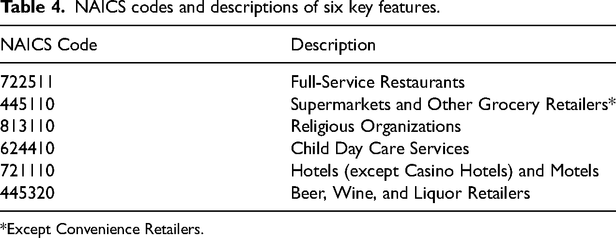
*Except Convenience Retailers.

Feature selection and eliminating abnormal entities also reduce the data points in this temporal dataset, making it feasible to utilize DC under MILP optimization, which guarantees globally optimal solutions and fully reproducibility results. The number of clusters $K$ was set to 3, determined by manually examining clustering results across candidate values ${3, 4, 5, 6}$ and drawing on insights from several related studies in Chicago (Delmelle 2016; Zhu et al. 2022). The selection was based on the criteria of low intra-cluster variance, where entities in each cluster exhibited distinct characteristics (i.e., low external cluster similarity), and all entities within each cluster could be accurately represented by the cluster definition (i.e., high internal cluster similarity). The maximum number of cluster label changes, $L$ , was set to 1 to identify the single neighborhood with the most divergent transition from its current temporal type.

To demonstrate the unique capabilities of DC, we applied the existing approach, which corresponds to SLA without limiting cluster label changes in our framework, under the same setting (i.e., $K = 3$ ) for comparative purposes. This dual approach enables us to evaluate the effectiveness of both SLA and DC in handling temporal data for neighborhood change analysis, given the same objective.¹⁷ Given that our primary goal in this paper is to examine the methodological implications of these different approaches of temporal clustering, we provide a relatively simple substantive analysis with few clusters and features. The primary result, as we will see, is that the statistical noise present in SLA, which arises from clustering time points independently, can potentially lead one to erroneously identify which neighborhoods exhibit high volatility in business patterns.

Cluster definitions using SLA

Recall that SLA disregards temporal relationships by clustering each time point independently. Applying SLA with a 3-cluster setting results in three static cluster definitions over time; each definition was obtained by aggregating all time points within this cluster using the mean (see Table 5).

Table 5.

Static cluster definitions for three neighborhood types using SLA the table below presents the values of the static definition for the three clusters (rows) across the six studied features (columns). These values represent the mean number of business establishments of different types across all time points within each cluster. Detailed descriptions of each neighborhood type are provided in the main manuscript. Analyses are based on SLA with $K = 3$ and $L = 1$ .

		Cluster Name (Neighborhood Types)
		Low Business Activity	Hotels and Restaurants	Daily Needs
Feature Name (Business Types)	Full-Service Restaurants	12.59	99.14	24.68
	Supermarkets and Grocery Store	9.70	19.73	27.58
	Religious Organizations	15.77	18.55	24.74
	Child Day Care Services	8.28	14.18	23.60
	Hotels (except Casino) and Motels	1.64	7.90	1.47
	Beer, wine, and liquor stores	4.12	8.15	7.83

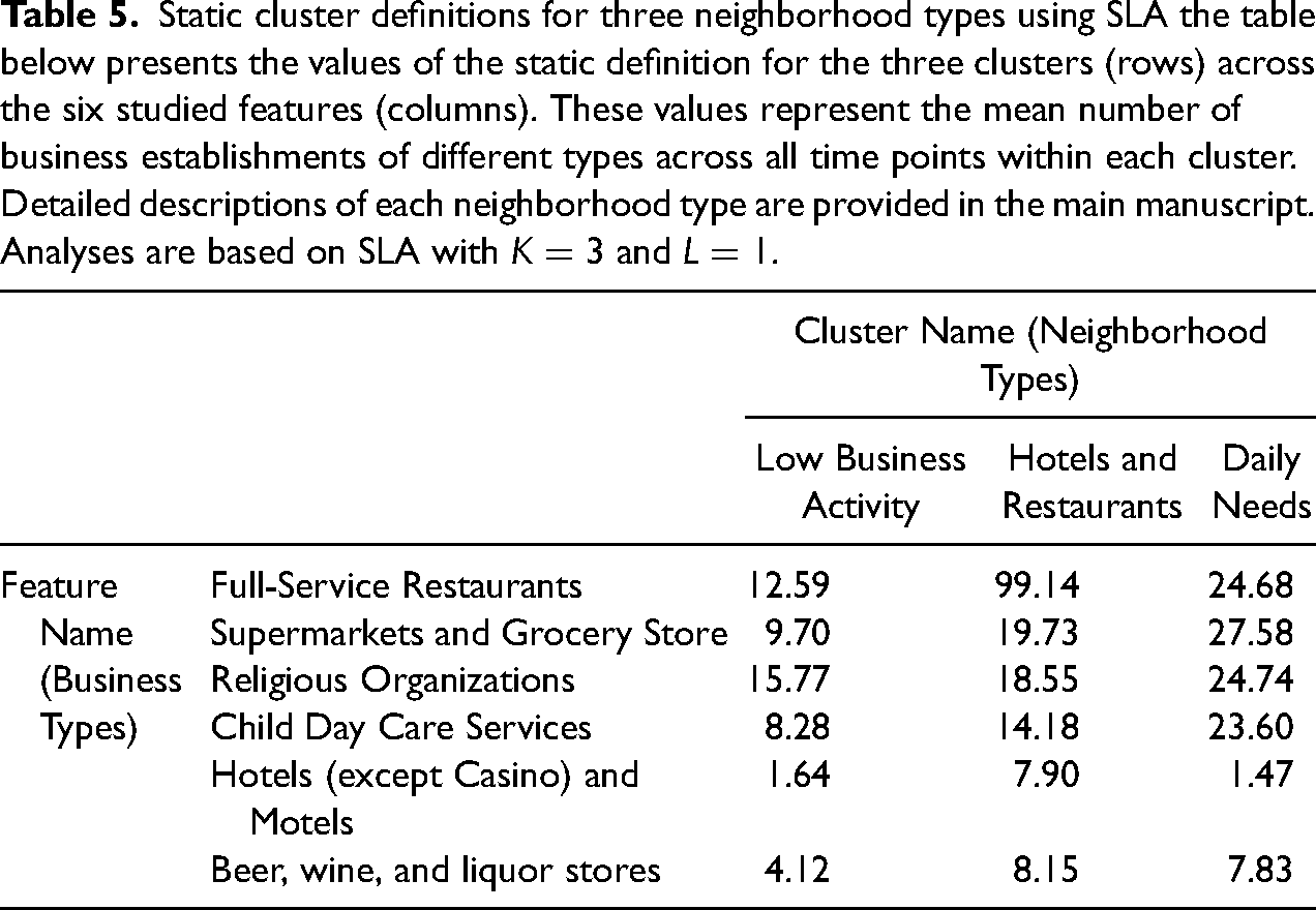
By analyzing the scores of the cluster definitions across different features, we identified the unique characteristics of each cluster based on their pattern of business establishments. Integrating with the spatial distribution of neighborhoods in each cluster (see Figure 11), the complete description of each cluster is stated below.

Low Business Activity: Neighborhoods in this cluster are characterized by having the lowest average number of business establishments across all six business types. Geographically, there is no distinct pattern in the spatial distribution of these neighborhoods, although some neighborhoods suggest that this cluster is located on the boundary of Chicago.

Hotels and Restaurants: This cluster exhibits the highest concentration of hotels, restaurants, and liquor stores relative to the other types. However, these neighborhoods lack establishments catering to daily needs, such as grocery stores and childcare facilities. These characteristics suggest a focus on services aimed at visitors rather than residents. These neighborhoods are concentrated north of the Loop, which includes several popular travel destinations such as Lincoln Park and Streeterville. This distribution further supports the hypothesis of a tourism-focused economic structure in these areas.

Daily Needs: Positioned in the outer regions of Chicago, this cluster is distinguished by having the highest number of business establishments focused on providing services for daily needs. In contrast to the Hotels and Restaurants cluster, this cluster is more oriented toward local residents based on these characteristics.

Figure 11.

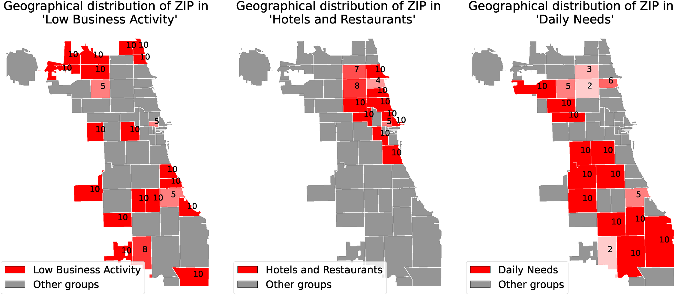
Geographical distribution of different neighborhood types using SLA. Given that neighborhoods’ cluster labels are dynamic, each neighborhood can belong to multiple clusters over time. The opacity of the choropleth map represents the frequency with which each neighborhood is assigned to a particular cluster. High opacity indicates that a neighborhood frequently belongs to this cluster, while low opacity suggests it is part of this cluster for a limited duration. The number of time points each neighborhood (minimum of one year) spends within this cluster is also annotated on the choropleth map. Hotels and Restaurants are predominantly concentrated in downtown Chicago, whereas Daily Needs establishments are primarily located in the outer regions. Although there is no clear concentration area for neighborhoods classified as Low Business Activity, some of these neighborhoods are located on the boundary of Chicago. Analyses are based on SLA with $K = 3$ and $L = 1$ .

As shown above, SLA can highlight important clusters in the data. However, the significant drawback of using SLA is its restriction that cluster definitions are temporally invariant, such that the characteristics of each cluster type consist of static comparisons rather than evolving patterns. For example, while SLA can identify that neighborhoods within the Hotels and Restaurants cluster tend to have more hotel-related business establishments than others, it does not account for whether this number increases over the years or if other business establishments remain constant or decline. Similarly, it cannot determine if neighborhoods in the Low Business Activity cluster consistently have lower numbers of all types of business establishments or if there is a shift from high to low starting from a particular time point.

Cluster definitions using DC

In contrast to SLA, DC utilizes dynamic cluster definitions, such that the cluster centers themselves are temporal trends (see Figure 12). The clustering results from DC, with $K = 3$ clusters and $L = 1$ cluster label change, modify the definitions of the three neighborhood types discussed in the previous section by incorporating the evolution of each type of business establishment over the years, as described below:

Low and Declining Business Activity: Besides having the lowest number of business establishments, this type of neighborhood shows declining trends in most business types. Specifically, the number of establishments within the “Beer, wine, and liquor stores” category declined from 2010 to 2016. The “Supermarket and grocery stores” category exhibited an increase until 2012, followed by a decline. Despite the spatial distribution being similar to that observed in SLA, there is a geographical concentration on the southeast side of Chicago (see the left choropleth map in Figure 13), including several community areas such as New City, which experienced a 15.6% population decline from 2000 to 2020, and Englewood, which saw a 39.4% population decline over the same period, both significantly higher than the 5.2% decline in Chicago overall (Chicago Metropolitan Agency for Planning 2023). Additionally, these neighborhoods have lower-than-average median incomes, which could contribute to the low and declining number of business establishments.

Stable Hotels and Restaurants: The number of hotel- and restaurant-related business establishments remains the highest among the three clusters, with numbers increasing over the years. For example, full-service restaurants exhibit a steady upward trend from 2007 to 2016, indicating robust growth in the tourism and hospitality sectors. By contrast, other business types have shown a declining trend over the years, suggesting that these neighborhoods are shifting toward a service-oriented profile. The exception is the “Beer, Wine, and Liquor Stores” category, which experienced a slight increase in 2010 before declining. The geographical distribution of neighborhoods in this cluster is more concentrated around the riverside area compared to SLA (see the middle choropleth map in Figure 13 and 11). By comparing them side by side, it is clear that the neighborhoods excluded from this cluster primarily include those that shifted between multiple clusters over time. Overall, DC captures those parts of Chicago exhibiting a clear movement toward a more post-industrial service and consumption orientation (Nichols Clark 2003).

Increasing Daily Needs: Despite the known prevalence of Daily Needs-related business establishments, the number of business establishments in the “Child Day Care Services” category has shown a significant increasing trend from 2007 to 2012, maintaining its dominance among the three clusters and highlighting the growing demand in this sector. Similar trends were observed for supermarkets and grocery stores. Although religious organizations remained the highest among all three types, there has been a declining trend since 2010, which may reflect broader socioeconomic or cultural shifts affecting these establishments. The geographical distribution of neighborhoods in this cluster (see right of Figure 13) is primarily in the outer and more residential regions of Chicago, divided into three sections: the far south side, parts of the southwest side, and the northwest side.

Figure 12.

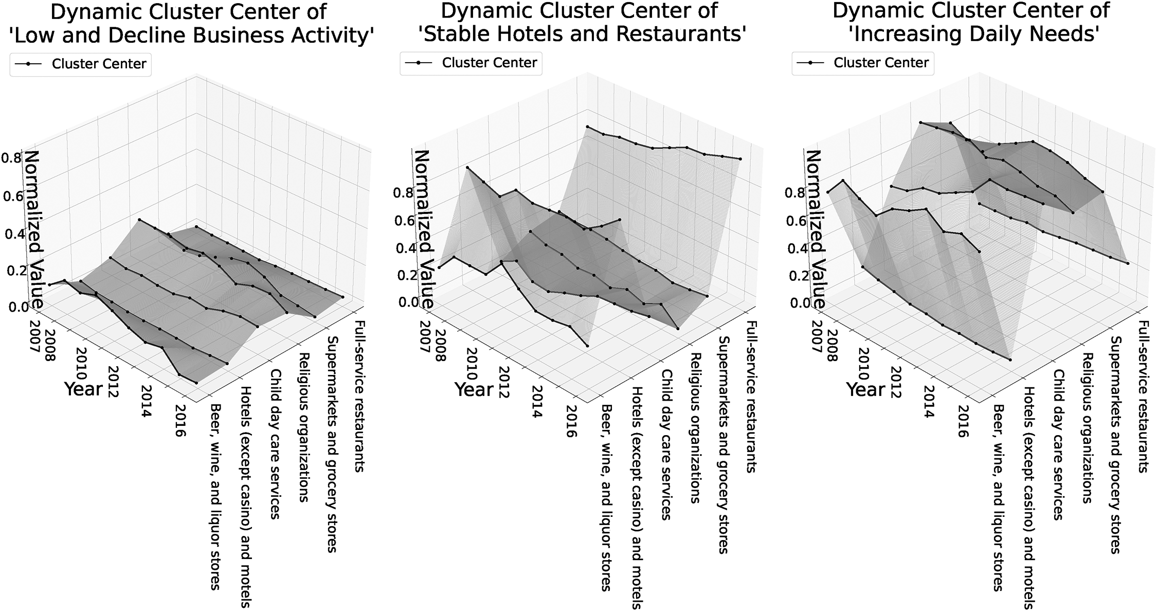
Definition of each neighborhood type using DC. Each of the three plots below illustrates the cluster definition of one of the neighborhood types when employing DC. In each plot, solid lines represent the values of business types (z-axis) after min–max normalization on each feature separately over various years (x-axis).¹⁸ Each line corresponds to a different type of business establishment. Analyses are based on DC with $K = 3$ and $L = 1$ .

Figure 13.

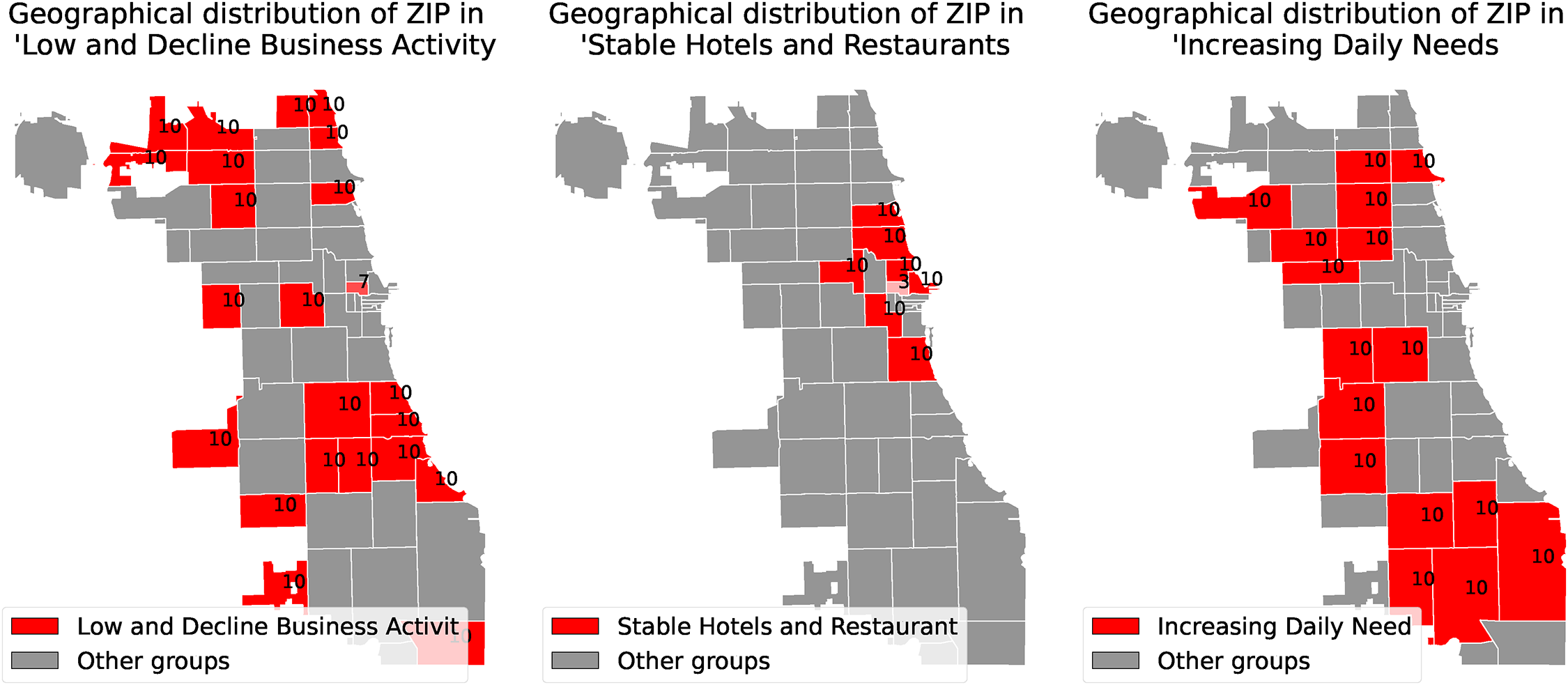
Geographical distribution of different neighborhood types using DC. The choropleth maps below depict the geographical distribution of neighborhoods within the three clusters identified by the DC clustering results. Each entity’s time points within the corresponding cluster are annotated on the choropleth maps. Analyses are based on DC with $K = 3$ and $L = 1$ . Note that, due to only one allowable change in entities’ label, most entities remain within a single cluster across all 10 time points.

Neighborhood volatility analysis

One of the key questions raised in neighborhood change research concerns the degree of volatility or continuity exhibited in different parts of a city (Silver and Silva 2021). A precondition to pursuing this question is the ability to reliably discern when a neighborhood is changing types. With SLA, a seemingly straightforward way to measure a neighborhood’s volatility is by counting the frequency of its label changes across the studied time points. More frequent changes indicate transitions between different neighborhood types, suggesting more volatility. In our 3-cluster SLA setting, eight entities experienced cluster label changes. ZIP 60643 stood out with four changes, alternating between Low Business Activity and Daily Needs clusters, making it the most frequently changing entity. However, a close examination of this case shows the limitations of existing SLA methods for identifying neighborhood volatility and the improved capacities offered by DC.

In fact, a thorough analysis of ZIP 60643’s temporal data (Figure 14) reveals no significant changes across the six considered features over time. The number of business establishments in “Child day care services” and “Supermarkets and grocery stores” shows contrasting values in the definitions of the two clusters to which ZIP 60643 was assigned. However, there are no substantial atypical trends that would justify these cluster label changes. This discrepancy suggests a potential misalignment between cluster labels and actual trends in the underlying features. One possible explanation for this misalignment is that ZIP 60643’s scores on these contrasting features lie on the boundaries between Low Business Activity and Daily Needs clusters, far from the centers of both clusters (Figure 15). This relative position makes ZIP 60643 vulnerable to statistical noise when clustering using conventional techniques, such as those commonly used in the literature on urban social change. 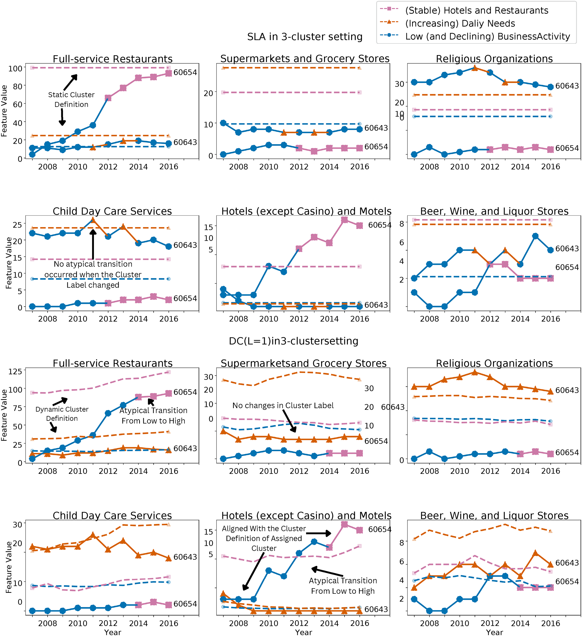Consequently, neighborhoods like ZIP 60643 may be incorrectly identified as an entity with atypical movements when using the conventional version of SLA, where $L$ is set to the maximum number of allowable cluster label changes.

Figure 14.

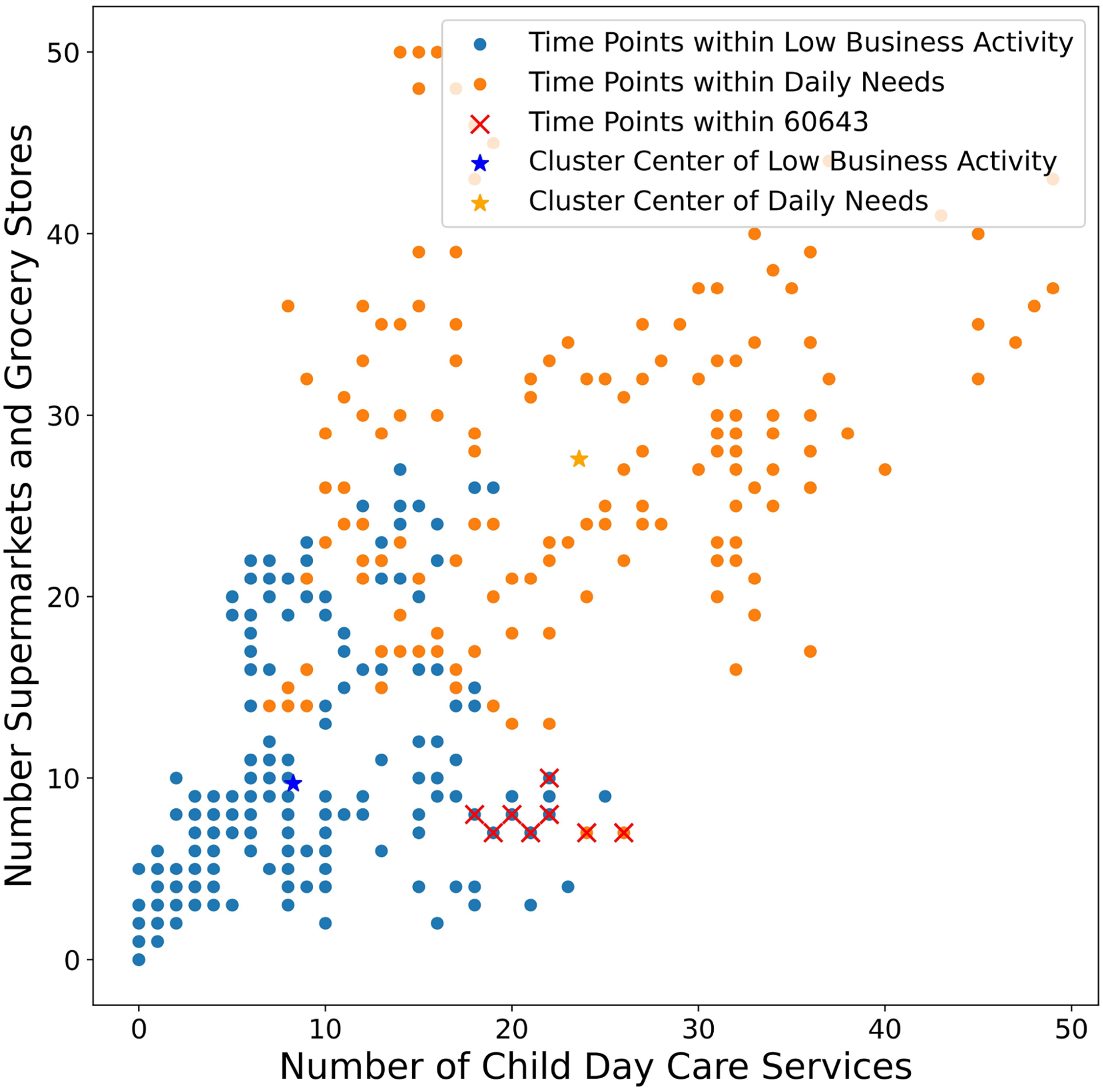
Neighborhood cluster label change using SLA (a) and (b) DC. These panels show line plots for the six features examined for two key neighborhoods. Specifically, the top panel (a) shows changes in the features for the most atypical cluster label change when using SLA with $K = 3$ and $L = 1$ . This was identified as ZIP 60643. By contrast, the bottom panel (b) shows the changes in the features for the most atypical cluster label change when using DC with $K = 63$ and $L = 1$ . This was identified as ZIP 60654. The color of the scatter plots and line segments indicates the cluster label of each entity at the corresponding time point. The dashed lines represent the cluster definitions, which are static in the top panel (a) but dynamic in the bottom panel (b).

Figure 15.

Scatter plot of two key features in two selected clusters. The scatter plot below illustrates the distribution of time points within the clusters Low Business Activity and Daily Needs across two features (labeled on each axis) that show contrasting values at the centers of these clusters (marked with a star). ZIP 60643, marked with a red cross, is located on the boundary between the two clusters, distant from the cluster centers. This position is susceptible to statistical noise in center-based clustering methods, potentially leading to erroneous identification of entities as frequently changing clusters.

By contrast, when we restricted the maximum allowable number of changes in entities’ label to one (i.e., $L = 1$ ) in DC, only ZIP 60654 underwent a change (Figure 14). Initially clustered within Low and Declining Business Activity, ZIP 60654 transitioned to the Stable Hotels and Restaurants cluster in 2014. The cluster definitions (Figure 12) highlight “Full-Service restaurants” and “Hotels (excluding casinos) and motels” as the distinguishing features between these two clusters. This transition underscores ZIP 60654’s unique business dynamics, evolving from a neighborhood with low business activity to one focused on service and tourism. ZIP 60654 encompasses the River North neighborhood of Chicago, located north of the Chicago River, including part of the Chicago Riverwalk, Merchandise Mart, and other attractions. A detailed analysis of the time series data for this entity reveals increasing trends in both full-service restaurants and hotels/motels (Figure 14). This significant increase can be attributed to various factors, including the Riverwalk expansion project initiated around 2011 (Hellenthal and Gross 2016). The impact of this development is reflected in the dramatic rise observed in the temporal data starting in 2011, leading to ZIP 60654’s cluster label change in 2014. It is worth noting that while ZIP 60654 also exhibits cluster label changes in SLA with $L$ set to the total number of possible changes, it is obscured among other changing entities. SLA would require a second-stage analysis to distinguish atypical change trends from misaligned entities like ZIP 60643. Moreover, note that by limiting the maximum number of changes to one in DC, the erroneously identified ZIP 60643 shows no label change (Figure 14).

The case studies in this section have demonstrated the utility of our unified framework for temporal clustering in providing new insights into various dimensions of social change. In the first case study, we analyzed a unique dataset of state-level opinions, policies, and political affiliations in the United States. Our method identified distinct temporal patterns that reveal increasing polarization in both political affiliation and the degree of liberalism in state policies and residents’ opinions. Moreover, by restricting the number of entities allowed to move across clusters, we were able to highlight those states with notable transitions that deviate from the broader shifts in cluster definitions. The second case study examined global cultural change using data from the WVS. Applying SLA, we developed a typology of cultural clusters that more closely aligns with the underlying survey indicators, in contrast to previous work ((e.g., see Inglehart 2006)). We also identified several countries, such as the United States and Pakistan, that have undergone significant cultural shifts and have moved from one cluster to another. Finally, in the third case study, we used historical data on business establishments in Chicago neighborhoods to identify distinct patterns of local economic development. By comparing our DC method to more conventional approaches, we demonstrated that the latter is prone to misidentifying atypical shifts arising from statistical noise. Taken together, these diverse applications illustrate the flexibility and insights gained from our unified framework for analyzing complex patterns of social change across a range of sociological contexts and scales.

Conclusion

The study of social change has long been hindered by overly simple theories and methods for joining concepts to data (Blumer 1990; Boudon 1986; Haferkamp and Smelser 1992; Lenski 2005; Tilly 1984). As Hallinan (1997)noted in her presidential address to the American Sociological Association, the field has often been constrained by unrealistic assumptions of “continuity, linearity, and stable equilibrium (2).” She urged sociologists to develop “new models that better portray and explain complex, contemporary social events (2).” This call for “new approaches to theories” to a classic sociological topic of social change Šubrt (2017) has been echoed more recently, highlighting a persistent need for better methodological tools (52).

Our unified framework for temporal clustering directly addresses these calls. By allowing for dynamic cluster definitions and for cases to transition between clusters, our approach moves beyond the limiting assumptions of linearity and continuity critiqued by Hallinan and others. Our paper makes five main contributions to the study of social change. First is the unified framework itself, which expands the methodological toolkit for analyzing complex units such as societies, neighborhoods, and states. By incorporating both evolving cluster definitions and assignments, our framework generalizes existing methods while offering new techniques such as DC, allowing researchers to select an approach suitable to their specific research questions and data.

Second, we formalize the objectives for temporal clustering, extending traditional center-based methods to incorporate an explicit temporal dimension. We provide mathematical objectives for each of the four main types in our framework, accommodating various combinations of static and dynamic cluster definitions and labels. This formalization provides a clear basis for comparing different clustering approaches and ensuring consistent and reproducible results.

Third, we develop new algorithmic methods, particularly for DC and SLA. These methods optimize clustering objectives while allowing researchers to constrain how many times a unit can change clusters. We also offer two complementary optimization techniques: Mixed Integer Linear Programming (MILP) methods, which provide globally optimal and reproducible solutions, and a more scalable iterative technique based on the MM algorithm, useful for larger datasets.

Fourth, we provide practical guidelines for applying temporal clustering in sociological research. These guidelines address key decisions in the research process, including feature selection, normalization, and the choice of an appropriate distance metric, number of clusters, and number of allowable label changes.

Finally, we illustrate our framework with three case studies that highlight the various ways in which our methods can be used in practice: first, an analysis of U.S. states identifies patterns of increasing political polarization and highlights several states that shift clusters over time; second, using the WVS, we develop a typology of cultural clusters and identify countries that transition between them; and, lastly, a study of business patterns in Chicago shows how our approach avoids the misidentification of atypical shifts that can arise from statistical noise in conventional methods.

Our framework has limitations that point to directions for future research. A key issue is the quantification of uncertainty due to random sampling. Our iterative MM-based algorithm, for instance, can produce locally optimal results that are not always reproducible, due to random initialization. While the MILP approach is globally optimal, it does not fully resolve the issue. Future research could address this by incorporating statistical inference methods such as bootstrapping into the clustering process to evaluate the statistical significance of the clustering results.

Another limitation is a reliance on $l_{1}$ (Manhattan distance) and $l_{2}$ (Euclidean distance) distance measures. While efficient, these metrics require units to have the same number of time points, necessitating pre-processing for some datasets, as in our state polarization case study. Future research could explore more flexible similarity metrics, such as DTW, which is better suited for comparing sequences of different lengths.

Scalability for very large datasets is another area for future work. Our framework presents a tradeoff between a globally optimal (MILP) approach that can be computationally intensive and an efficient (MM-based) method that may be more scalable but less optimal. Future research could focus on developing hybrid methods to better balance this trade-off. Possibilities include machine learning techniques for data reduction or feature extraction, parallel computing strategies for MILP optimization, or advanced heuristics that approximate global optima more closely than current MM-based methods.

Finally, our framework’s applications extend beyond the geographical cases presented here. Our approach can be generalized to any feature space with a meaningful order, such as occupational hierarchies, educational levels, or socioeconomic strata. This allows for studying social mobility where the units represent positions in a social hierarchy. The framework is also well-suited for cohort analysis, where units can represent different birth cohorts, making it possible to track generational change (Fosse 2023a; Waite et al. 2021). While such applications require careful thought about defining similarity in abstract spaces, they highlight the broader potential of temporal clustering in sociological research.

Supplemental Material

sj-pdf-1-smr-10.1177_00491241251396789 - Supplemental material for Mapping Social Change: A Unified Framework for Temporal Clustering

Supplemental material, sj-pdf-1-smr-10.1177_00491241251396789 for Mapping Social Change: A Unified Framework for Temporal Clustering by Jiazhou Liang, Jolomi Tosanwumi, Ethan Fosse, Daniel Silver and Scott Sanner in Sociological Methods & Research

Footnotes

Declaration of Conflicting Interest

The authors declared no potential conflicts of interest with respect to the research, authorship, and/or publication of this article.

Funding

The authors received no financial support for the research, authorship, and/or publication of this article.

Preregistration Statement

This study was not preregistered, as all datasets used are either publicly available or accessible with restrictions from third parties, and existed before the beginning of this research.

ORCID iDs

Jiazhou Liang

Ethan Fosse

Daniel Silver

Scott Sanner

Data,Code,and Materials Availability Statement

The datasets generated during and/or analyzed during the current study are available in the .

Supplemental Material

Supplemental material for this article is available .

Notes

Author Biographies

Jiazhou Liang is a Master’s student in Industrial Engineering at the University of Toronto. Jiazhou’s research is focused on a wide range of data science applications and machine learning methodologies.

Jolomi Tosanwumi is a Master’s student in Industrial Engineering at the University of Toronto. His research focuses on data science and machine learning techniques and their applications.

Ethan Fosse is an Associate Professor of Sociology, Associate Director of the Data Sciences Institute, and Faculty Affiliate with the Centre for Analytics and Artificial Intelligence Engineering at the University of Toronto.

Daniel Silver is a Professor of Sociology at the University of Toronto.

Scott Sanner is a Professor in Industrial Engineering and Cross-appointed in Computer Science at the University of Toronto. His research spans topics including data science, machine learning, and AI.

References

Aghabozorgi

Saeed

Shirkhorshidi

Ali Seyed

Wah

Teh Ying

. 2015. “Time-Series Clustering—A Decade Review.” Information Systems 53: 16–38.

Aisenbrey

Silke

Fasang

Anette E.

. 2010. “New Life for Old Ideas: The “Second Wave” of Sequence Analysis Bringing the “Course” Back Into the Life Course.” Sociological Methods & Research 38: 420–462.

Blumer

Herbert

. 1990. Industrialization As An Agent of Social Change: A Critical Analysis. New York, NY: Routledge.

Boudon

Raymond

. 1986. Theories of Social Change: A Critical Appraisal. Berkeley, CA: University of California Press.

Brown

Jacob R.

Enos

Ryan D.

. 2021. “The Measurement of Partisan Sorting for 180 Million Voters.” Nature Human Behaviour 5: 998–1008.

Bureau. 2023. “United States Census.” ZIP Codes Business Patterns (ZBP) APIs.

Carrillo

Humberto

Lipman

David

. 1988. “The Multiple Sequence Alignment Problem in Biology.” SIAM Journal on Applied Mathematics 48: 1073–1082.

Caughey

Devin

Warshaw

Christopher

. 2018. “Policy Preferences and Policy Change: Dynamic Responsiveness in the American States, 1936-2014.” American Political Science Review 112: 249–266.

Chembu

Aravinth

Sanner

Scott

Khurram

Hassan

Kumar

Akshat

(2023) “Scalable and Globally Optimal Generalized L1 K-Center Clustering via Constraint Generation in Mixed Integer Linear Programming.” pp. 7015-7023 in Proceedings of the AAAI Conference on Artificial Intelligence, Vol. 37.

10.

Chiang

Mark

Mirkin

Boris

. 2010. “Intelligent Choice of the Number of Clusters in K-Means Clustering: An Experimental Study With Different Cluster Spreads.” Journal of Classification 27: 3–40.

11.

Chicago Metropolitan Agency for Planning. 2023. “Chicago Metropolitan Agency for Planning’s Community Data Snapshots July 2023 Release.” [Online; accessed 26. Jun. 2024].

12.

Delmelle

Elizabeth C.

2015. “Five Decades of Neighborhood Classifications and Their Transitions: A Comparison of Four US Cities, 1970-2010.” Applied Geography 57: 1–11.

13.

Delmelle

Elizabeth C.

2016. “Mapping the DNA of Urban Neighborhoods: Clustering Longitudinal Sequences of Neighborhood Socioeconomic Change.” Annals of the American Association of Geographers 106: 36–56.

14.

Delmelle

Elizabeth C.

2017. “Differentiating Pathways of Neighborhood Change in 50 US Metropolitan Areas.” Environment and Planning A 49: 2402–2424.

15.

Dias

Fabio

Silver

Daniel

. 2021. “Neighborhood Dynamics with Unharmonized Longitudinal Data.” Geographical Analysis 53: 170–191.

16.

Fonseca

Jaime R. S.

2013. “Clustering in the Field of Social Sciences: That is Your Choice.” International Journal of Social Research Methodology 16: 403–428.

17.

Fosse

Ethan

. 2023a. “Dissecting the Lexis Table: Summarizing Population-Level Temporal Variability with Age–Period–Cohort Data.” Sociological Science 10: 150–196.

18.

Fosse

Ethan

. 2023b. “Theorizing in the Cohort Mode: On Ryder’s Processual Account of Social Change.” Canadian Studies in Population 50: 5.

19.

Fosse

Ethan

. 2023c. “Visualizing Social Change with Ryder Plots: The Rise and Fall of Verbal Ability in the United States.” Socius 9: 23780231231197302.

20.

Fosse

Ethan

Winship

Christopher

. 2023. “The Anatomy of Cohort Analysis: Decomposing Comparative Cohort Careers.”Sociological Methodology 53:217–268.

21.

Grossmann

Matt

Jordan

Marty P.

McCrain

Joshua

. 2021. “The Correlates of State Policy and the Structure of State Panel Data.” State Politics & Policy Quarterly 21: 430–450.

22.

Haerpfer

Christian

Inglehart

Ronald

Moreno

Alejandro

Welzel

Christian

Kizilova

Kseniya

Diez-Medrano

Jaime

Lagos

Marta

et al. 2022. “World Values Survey Time-Series (1981-2022) Cross-National Data-Set.”

23.

Haferkamp

Hans

Smelser

Neil J.

. 1992. Social Change and Modernity. Berkeley, CA: University of California Press.

24.

Hallinan

Maureen T.

1997. “The Sociological Study of Social Change.” American Sociological Review 62: 1–11.

25.

Hellenthal

Matthew F.

Gross

Dan M.

. 2016. Design and Construction of the Chicago Riverwalk. Reston: American Society of Civil Engineers.

26.

Hernes

Gudmund

Land

Kenneth C.

. 2015. “Social Changes: Models.” pp. 192-198 in International Encyclopedia of the Social & Behavioral Sciences, edited by James D. Wright.

27.

Huntington

Samuel P.

2020. “The clash of civilizations?” pp. 305-313 in The new social theory reader. Routledge.

28.

Inglehart

Ronald

. 2006. “Mapping Global Values.” Comparative Sociology 5: 115–136.

29.

Iyengar

Shanto

Lelkes

Yphtach

Levendusky

Matthew

Malhotra

Neil

Westwood

Sean J.

. 2019. “The Origins and Consequences of Affective Polarization in the United States.” Annual Review of Political Science 22: 129–146.

30.

Kang

Wei

Rey

Sergio

Wolf

Levi

Knaap

Elijah

Han

. 2020. “Sensitivity of Sequence Methods in the Study of Neighborhood Change in the United States.” Computers, Environment and Urban Systems 81: 101480.

31.

Kenneth

Lange

Hunter

David R.

Yang

Ilsoon

. 2000. “Optimization Transfer Using Surrogate Objective Functions.” Journal of Computational and Graphical Statistics 9: 1–20.

32.

Kodinariya

Trupti M.

Makwana

Prashant R.

. 2013. “Review on Determining Number of Cluster in K-Means Clustering.” International Journal 1: 90–95.

33.

Lenski

Gerhard

. 2005. Ecological-Evolutionary Theory Principles and Applications. Boulder, CO: Paradigm Publishers.

34.

Levine

Joel H.

2000. “But What Have You Done for Us Lately? Commentary on Abbott and Tsay.” Sociological Methods & Research 29: 34–40.

35.

Liang

Jiazhou

Jolomi

Tosanwumi ,

Ethan

Fosse ,

Daniel

Silver , and

Scott

Sanner . 2025 Data and Code Release for “Mapping Social Change: A Unified Framework for Temporal Clustering.” 10.5281/zenodo.16923545.

36.

Liao

T. Warren

. 2005. “Clustering of Time Series Data—A Survey.” Pattern Recognition 38: 1857–1874.

37.

Ling

Chenjun

Delmelle

Elizabeth C.

. 2016. “Classifying Multidimensional Trajectories of Neighbourhood Change: A Self-Organizing Map and K-Means Approach.” Annals of GIS 22: 173–186.

38.

Lloyd

1982. “Least Squares Quantization in PCM.” IEEE Transactions on Information Theory 28: 129–137.

39.

McCarty

Nolan

Poole

Keith T.

Rosenthal

Howard

. 2016. Polarized America: The Dance of Ideology and Unequal Riches. Cambridge: MIT Press.

40.

Meagher

Kelsey D.

Shu

Xiaoling

. 2019. “Trends in U.S. Gender Attitudes, 1977 to 2018: Gender and Educational Disparities.” Socius 5: 1–3.

41.

Müller

Meinard

. 2007. Information Retrieval for Music and Motion. Berlin: Springer Science & Business Media.

42.

Nichols Clark

Terry

. 2003. The City As An Entertainment Machine. Leeds: Emerald Group Publishing Limited.

43.

Patias

Nikos

Rowe

Francisco

Cavazzi

Stefano

. 2020. “A Scalable Analytical Framework for Spatio-Temporal Analysis of Neighborhood Change: A Sequence Analysis Approach.” pp. 223-241 in Geospatial Technologies for Local and Regional Development: Proceedings of the 22nd AGILE Conference on Geographic Information Science 22, Springer.

44.

Poole

Keith T.

Rosenthal

Howard

. 1984. “The Polarization of American Politics.” The Journal of Politics 46: 1061–1079.

45.

Rousseeuw

Peter J.

Kaufman

Leonard

. 2009. Finding Groups in Data: An Introduction to Cluster Analysis. Hoboken, NJ: John Wiley & Sons.

46.

Shieh

Jin

Keogh

Eamonn

. 2008. “i SAX: Indexing and Mining Terabyte Sized Time Series.” pp. 623-631 in Proceedings of the 14th ACM SIGKDD international conference on Knowledge discovery and data mining.

47.

Silver

Daniel

Adler

Patrick

Fox

Mark S.

. 2022a. “Towards a Model of Urban Evolution-part I: Context.” Urban Science 6: 87.

48.

Silver

Daniel

Silva

Thiago H.

. 2021. “A Markov Model of Urban Evolution: Neighbourhood Change As a Complex Process.” PloS one 16: e0245357.

49.

Silver

Daniel

Silva

Thiago H.

. 2023. “Complex Causal Structures of Neighbourhood Change: Evidence From a Functionalist Model and Yelp Data.” Cities (London, England) 133: 104130.

50.

Silver

Daniel

Silva

Thiago H.

Adler

Patrick

. 2022b. “Changing the Scene: Applying Four Models of Social Evolution to the Scenescape.” arXiv preprint arXiv:2209.10665.

51.

Silver

Daniel Aaron

Clark

Terry Nichols

. 2016. Scenescapes: How Qualities of Place Shape Social Life. Chicago: University of Chicago Press.

52.

Small

Mario Luis

McDermott

Monica

. 2006. “The Presence of Organizational Resources in Poor Urban Neighborhoods: An Analysis of Average and Contextual Effects.” Social Forces 84: 1697–1724.

53.

Steinley

Douglas

. 2003. “Local Optima in K-Means Clustering: What You Don’t Know May Hurt You.” Psychological Methods 8: 294.

54.

Stone

Emily

Cutler

Adele

. 1996. “Introduction to Archetypal Analysis of Spatio-Temporal Dynamics.” Physica D: Nonlinear Phenomena 96: 110–131.

55.

Šubrt

Jiří

. 2017. The Perspective of Historical Sociology: The Individual As Homo-Sociologicus Through Society and History. Bingley, UK: Emerald Publishing.

56.

Tilly

Charles

. 1984. Big Structures, Large Processes, Huge Comparisons. New York, NY: Russell Sage Foundation.

57.

Waite

Linda J.

Hawkley

Louise

Kotwal

Ashwin A.

O’Muircheartaigh

Colm

Schumm

Philip L

Wroblewski

Kristen

. 2021. “Analyzing Birth Cohorts With the National Social Life, Health, and Aging Project.” The Journals of Gerontology: Series B 76: S226–S237.

58.

Yuan

Chunhui

Yang

Haitao

. 2019. “Research on K-Value Selection Method of K-means Clustering Algorithm.” J 2: 226–235.

59.

Zhu

Qing

Zhang

Fan

Liu

Shan

Yuze

. 2022. “An Anticrime Information Support System Design: Application of K-Means-VMD-BiGRU in the City of Chicago.” Information & Management 59: 103247.