



Abstract

This comment will focus on the use of three strategies identified by Robette, Bry, and Lelièvre (this volume, pp. 1–44; hereafter RBL)—namely, globally interdependent multiple sequence analysis (GIMSA), multichannel sequence analysis (MCSA), and FS, the so-called fourth strategy (clustering sequences separately and analyzing their relationship afterward). I address more specifically the question of their usefulness for analyzing the relationships between different kinds of trajectories. Meanwhile, I identify possible directions for future research and propose some new tools.
While giving sequence analysis (SA) courses or answering TraMineR-related questions, I have noticed frequent confusion about the goal of cluster analysis (CA), which I would like to clarify here. Because the three aforementioned strategies are based on CA, this discussion is also relevant for our topic.
CA aims to reveal the structure of data by looking at patterns of answers—that is, configurations of the values taken by the included variables. However, this is very different from looking at the relationships among the included dimensions.
Let me briefly present the difference between the two, using a simple example. Suppose we want to analyze two ordinal variables, say x and y, with the joint and marginal distributions shown in Table 1.
Joint and Marginal Distributions of Two Ordinal Variables, x and y
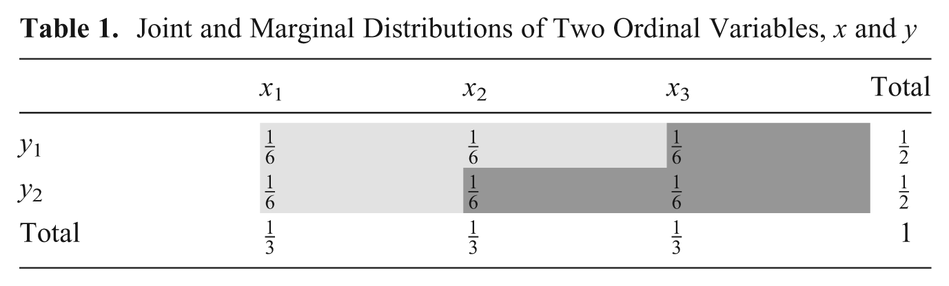
In this example, patterns are identified by looking at the joint distribution. For this reason, a six-cluster solution would be a good one according to most indices of clustering quality (e.g., Studer 2013), even if there is no association between x and y. In order to interpret the relationship between x and y, we usually look at the conditional distributions, which tell us whether each value of x is associated with a different distribution of y. We may be able to deduce the association by comparing the joint distribution with the marginal ones. However, this soon becomes a difficult task when using CA, because CA may well regroup cells irrespective of their rows and columns. In that case, we would lack a reference model (such as statistical independence) to determine whether there is an association and to interpret the form of this association.
Using CA to analyze the relationship between two (or more) variables is also risky because the reduction of information made by CA can potentially lead to wrong conclusions. For instance, suppose that we retained a two-cluster solution according to the gray scale in our previous example. We could well think that higher values of x imply higher values in y, which is wrong here. Following a similar reasoning, CA can hide a significant association between two (or more) variables.
Hence, a good clustering is not a sign of a relationship between the variables, but rather it is a sign of homogeneous and well-separated configurations of answers. In other words, clustering cannot be used to test or to interpret the form of an association. This is why we should always use a proper test to confirm an association identified using CA.
Does this mean that CA is useless? Of course not. CA can be used to build a typology involving several indicators (or subdimensions) of a given dimension. Because these indicators measure a unique dimension, a typology can be useful to regroup them in only one construct in subsequent analysis. In this case, we make the assumption—and we should justify it sociologically—that these indicators are intrinsically related. Furthermore, in this case, the relationship between the indicators is not the primary interest, or it is analyzed separately. For all these reasons, CA is of interest when looking at one concept or dimension, without being primarily interested in the relationship between the variables or indicators.
What does it imply for SA, GIMSA, MCSA, and FS? For the SA case, Abbott (1992) justified on a theoretical ground the need to analyze trajectories and processes as a whole in order to take their internal logic into account without making too many assumptions on the generating process. However, if important relationships between different moments of the trajectories have been identified using CA, I would still recommend using a specific test to confirm the relation.
In FS, sequences are clustered separately before analyzing the relationship. Hence, the relationship can then be analyzed safely using any categorical data analysis methods. 1 RBL use, for instance, a crosstable to comment on the results (see Table 2 in their article). As noted by RBL, we observe a significant but weak (Cramer’s v = .094) relationship between the two kinds of trajectories. A more detailed interpretation of the results can be made by looking at standardized Pearson residuals of the crosstable, as presented in Table 2.
Standardized Pearson Residuals of the Contingency Table of Daughters’ (Rows) and Mothers’ (Columns) Trajectories

Note: Residuals less than −1.96 can be interpreted as underrepresentation and those higher than 1.96 as overrepresentation of a configuration (Agresti 1990). FT = full-time; PT = part-time.
We observe some kind of “inactivity transmission,” because daughters with mothers who follow “mostly inactive” trajectories have more chances to be “mostly inactive” themselves. Furthermore, as noted by RBL, daughters following “mostly part-time” trajectories have more often than expected in the independence case mothers with “mostly high or intermediate” trajectories.
MCSA and GIMSA cannot be used to describe how two (or more) sequences are interrelated, nor can it be used at a local or at a global level. The obtained frequencies of the clusters are difficult to interpret, because we lack the marginal distributions or a reference model that would allow us to interpret the association. In other words, in GIMSA, we do not know what would be the result of the analysis without an association between daughters’ and mothers’ trajectories, making it very difficult to interpret the relationship between the two. 2
However, MCSA is useful when a trajectory is measured using different subdimensions—that is, when these subdimensions are studied as a unique concept. For instance, trajectories of hierarchical job positions and firm sizes could be grouped to analyze professional careers. Here again, the relationship between the sequences is not of primary interest.
GIMSA could be of interest if the trajectories under study are different subdimensions of the same concept and if we are not interested in the relationships between these trajectories. Rightly, RBL claim that they are interested in finding the frequent patterns of mother-daughter trajectories, not their relationships. However, when interpreting the results, they soon start interpreting the relationships between the two trajectories by saying that “mothers’ inactivity is often linked to daughters’ inactivity (and mothers’ activity to daughters’ full-time employment.” As we have shown earlier, such a statement cannot be made safely using CA, and hence GIMSA.
In order to analyze a relationship globally (i.e., without being interested in the local or contemporaneous interdependencies), several other strategies are available. Let me illustrate them using the mother-daughter example. We can cluster mothers’ trajectories and look at how much the mother clusters explain the discrepancy of daughters’ trajectories using discrepancy analysis (Studer et al. 2011). Here again, we find a significant but weak association (pseudo-R2 of about 1 percent).
Finally, we can have a more precise understanding of how daughters’ trajectories differ according to the typology of mothers’ trajectories by looking at the “sequences of typical states” (Studer 2012). Figure 1 presents the “sequences of typical states,” visualizing the differences between two or more groups of trajectories. It presents at each time point the typical states of a subpopulation (here according to mothers’ trajectories) using implicative statistics, which assess the statistical relevance of a rule of the form “A implies B.” 3
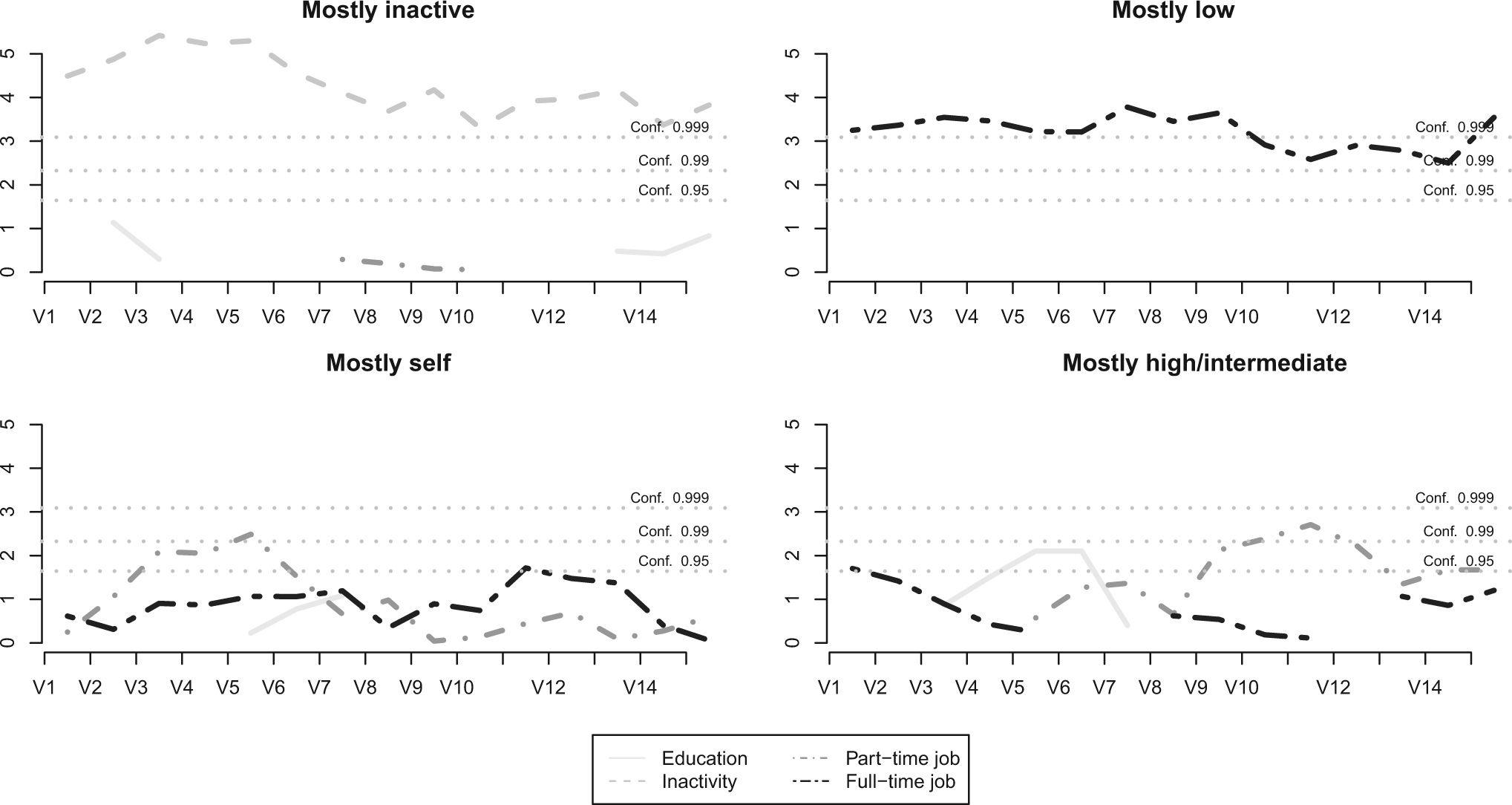
A sequence of typical states of daughters according to the typology of mothers’ trajectories.
The “mostly inactive” graph in Figure 1 presents at each time point t the relevance of the rule “Having a mostly inactive mothers’ trajectory implies being in state A at time t.” The horizontal dashed lines present the confidence thresholds. A rule is considered statistically significant at the 5 percent level if it exceeds the 95 percent confidence horizontal line. 4 Here, we can see that having a mostly inactive mothers’ trajectory implies being inactive, and this rule is significant for the whole daughters’ trajectory. Interestingly, some rules are significant for only a given period. Having “mostly high or intermediate” mothers’ trajectories implies being in education in the beginning of the trajectories (but not later) and being in part-time employment afterward (as noted already by RBL).
This “sequence of typical states” figure can be extended to analyze local relationships. We can look at the typical states of sequence B at time t (daughters) according to the state of sequence A at time t (i.e., mothers). Such a method should allow the study of how the relationship among trajectories evolves over time.
Before concluding, I would like to discuss one final issue. If we use CA to cluster different dimensions and cross-tabulate them with a factors of interest such as cohort, we presuppose an interaction effect. But the relationship might also result from a direct effect. A more parsimonious approach would start by analyzing direct effects and include the interaction term only if it is relevant.
For instance, RBL’s Appendix E analyzes how transmission patterns are related to factors such as the daughter birth cohorts. RBL found that the “inactivity transmission” pattern was more frequent in older daughters’ birth cohorts than in younger ones. By doing so, they presume an interaction effect between daughters’ and mothers’ trajectories and daughters’ birth cohorts. But this relation may well hide a direct effect. 5 GIMSA does not allow studying the direct effects—because we have only a joint typology—whereas FS (clustering sequences separately) allows this to happen.
In conclusion, I want to clarify a common confusion about the purpose of CA that may well affect GIMSA as well. CA should not be used to interpret or test a relationship, and the same applies to GIMSA. Even if some workarounds are available, we still need a proper method to do it, on a global as well as a local level.
Footnotes
Funding
The author disclosed receipt of the following financial support for the research, authorship, and/or publication of this article: This comment benefited from the support of a postdoctoral fellowship and from the Swiss National Centre of Competence in Research LIVES—Overcoming Vulnerability: Life Course Perspectives, both granted by the Swiss National Science Foundation. The author is grateful to the foundation for its financial assistance.