Model Misspecification When Eliminating a Factor in Age-period-cohort Multiple Classification Models

Abstract

The impossibility of uniquely estimating all of the age, period, and cohort coefficients in age-period-cohort multiple classification (APCMC) models without imposing a constraint on the model is widely recognized. The problem results from a linear dependency in the design matrix, and this dependency involves the linear trends of age effects, period effects, and cohort effects. This article critiques the use of fit statistics to assess the overall importance of the effects of ages, periods, and cohorts in APCMC models. In particular, one proposed strategy to avoid the APCMC model identification problem is to test to see if including only two of the factors in a model (e.g., ages and cohorts) produces a fit that is not significantly different statistically from a model that includes all three factors. If the third factor (in this example periods) does not account for a statistically significant amount of variance, this strategy suggests that one should use the model with only the two factors. This is consistent with model selection approaches. The two-factor model is identified and produces estimates of the individual effects of ages and cohorts. There is, however, a fundamental problem with this approach when used with APCMC models. That problem results from the complete confounding of the linear effects of the three factors.

Keywords

age-period-cohort models linear confounding variable selection eliminating factors

1. Introduction

For decades, researchers have known that it is not possible to separate the effects of ages, periods, and cohorts in a straightforward manner since they are intrinsically confounded (Mason et al. 1973; Schaie 1965). Schaie (1965), Mason et al. (1973), and other researchers consider a particular parameterization of this problem: the age-period-cohort multiple classification (APCMC) model. In this parameterization, each of the ages, periods, and cohorts are coded categorically (with a single category for each of these factors serving as reference categories). I will focus on this parameterization, which is widely used in the literature.

The most popular solution to this confounding problem (identification problem) places a single constraint on a model that contains all three factors; for example, the first age-group coefficient equals the second age-group coefficient or the linear trend for the period coefficients is zero. The single just-identifying constraint produces a solution for the age, period, and cohort coefficients under the constraint.¹ Unfortunately, there is an infinite number of these solutions that fits the data equally well, and these solutions can differ considerably depending on the constraint used. Only if the constraint is consistent with the age, period, and cohort parameters that generated the data will the coefficients under the constraint be unbiased estimates of the data-generating parameters. When using this method, we should use theory/substantive knowledge to set a constraint that is more likely to be close to the parameters that generated the data.²

The incremental factor fit strategy, which is the focus of this article, does not depend on theory/substantive knowledge. It eliminates one of the factors (ages, periods, or cohorts) if that factor does not make the model fit significantly better statistically when added to a model containing the other two factors. In the ordinary least squares (OLS) situation, we could compute $R^{2}$ for the three-factor model $(R_{three factors}^{2})$ and then run a regression model with just two of the factors ( $R_{two factors}^{2}$ ).³ If the increment in $R^{2}$ due to the third factor ( $R_{increment}^{2} = R_{three factors}^{2} - R_{two factors}^{2}$ ) is not statistically significant, researchers often conclude that the third factor is not important and can be left out of the model with little or no harm. This is a typical variable selection approach. It creates an atheoretical solution to the APC identification problem since any just-identifying constrained three-factor solution produces the same $R_{three factors}^{2}$ , and if the three-factor model fit is not significantly better statistically than the two-factor model, the two-factor model serves as the solution to the APC identification problem.⁴

The same rationale is used for generalized linear models (GLM), although the criterion differs. Typically, one would calculate the likelihood ratio chi-square: $- 2 \times [ln (likelihood of two factor model) - ln (likelihood of the three factor model)] .$ This likelihood ratio chi-square ( $G^{2}$ ) serves as a significance test for the contribution to the fit of the model of the third factor. If this test does not reject the null hypothesis of no statistically significant improvement in the fit of the model by the third factor, researchers would often drop the third factor.⁵

These incremental fit tests, using OLS or GLM, are employed by many authors working in the APC tradition; for example, see Clayton and Schifflers (1987b); Greenberg and Larkin (1985); Hall, Mairesse, and Turner (2005); Phillips (2014); Shahpar and Li (1999); and Yang and Land (2013). Working with just two of the factors identifies what otherwise (without a constraint) would be an unidentified model.⁶

2. Incremental Fit Tests of Factors in APCMC Models

Although it is known that the linear trends of the categorical effect coefficients for ages, periods, and cohorts are linearly dependent (Holford 1983; Luo 2013; O’Brien 2011b), the implications of this dependence are often overlooked when it comes to employing incremental fit tests for the overall importance of ages, periods, and cohorts. Recently Yang and colleagues (Yang et al. 2008; Yang, Fu, and Land 2004; Yang and Land 2013) suggested that such tests should be conducted before deciding to use the intrinsic estimator (IE). Yang and Land (2013:107) state:

One way to select among models is to conduct model fit tests of whether all three of the A, P, and C effects are present and should be simultaneously estimated (e.g., see Mason and Smith 1985). That is, analysts should successively estimate models with A, P, C, AP, AC, PC, and APC sets of effect coefficients and examine the corresponding model fit statistics for improvement as additional sets of combinations of coefficients are added. This gives a sense of the relative importance of A, P, C, effects and the best models that summarize the trends in the observed data.

They conclude: “We reiterate that imposition of a full APC model on data when a reduced model fits the data equally well or better constitutes a model misspecification and should be avoided” (Yang and Land 2013:109).

Yang, Land, and colleagues are not alone in advocating the incremental fit tests for the two- and three-factor models. Clayton and Schifflers (1987a, 1987b) in epidemiology and Hall et al. (2005) in economics provide two other prominent examples. As noted previously, many other authors have used this approach to identify APCMC models.

The problem with such solutions derives from the confounding of the linear trends of the three factors: age, period, and cohort. To explain the operational meaning of linear trends in the APCMC context, I use the age-factor as an example. To obtain the linear trend for ages, regress the age effect coefficients (based on one of the just-identifying constrained solutions) from the youngest to the oldest age group on $i = 1$ to $I$ , where $I$ is the number of age groups. A similar procedure can be used to calculate the trend for periods from the earliest to the most recent period and for cohorts from the earliest to the most recent cohort for that same constrained solution. These linear trends differ depending on the constraints used to identify the model. It is important to note that these linear trends are based on the coefficients associated with the APCMC model that is the focus of this article: They might arise from a curvilinear data-generating effect, but the confounding in the model will still exist.⁷ Because of the categorical coding of the age, period, and cohort effects in APCMC models, any linear trend of the left-out factor is attributed to the other two factors in a model. Table 1 summarizes this problem.

Table 1.

Explicit and Estimated Model $R^{2}$ and the Assumptions Associated with the Explicit Model for the Standard Age-period-cohort Multiple Classification (APCMC) Approach When Dropping a Factor

APCMC Approach When Dropping a Factor	Explicit Model	Captured by Model	Assumptions about the Left-out Factor When It Is Dropped from the Model
Age-period model	$R_{AP}^{2}$	$R_{AP (C_{L})}^{2}$	Linear and nonlinear effects equal zero $coh 1 = coh 2 = \dots = cohK = 0$
Age-cohort model	$R_{AC}^{2}$	$R_{AC (P_{L})}^{2}$	Linear and nonlinear effects equal zero $per 1 = per 2 = \dots perJ = 0$
Period-cohort model	$R_{PC}^{2}$	$R_{PC (A_{L})}^{2}$	Linear and nonlinear effects equal zero $age 1 = age 2 = \dots = ageI = 0$

Table 1 uses $R^{2}$ notation to show the amount of variance in the dependent variable that is explicitly accounted for (column 2) by different two-factor models (column 1) and the amount that is actually accounted for (captured) by the model (column 3). We could write analogous notation for GLM models. For the standard APCMC model with cohort as the left-out factor, the explicit model specifies just the two main effects ( $R_{AP}^{2}$ ) by including the categorically coded variables for ages and periods. This estimated model, however, accounts for the two main effects and any linear effects of the third factor ( $R_{AP (C_{L})}^{2}$ ). The increment in $R^{2}$ F-test using the standard approach tests only whether the nonlinear effects (deviations from the linear trend) associated with the third factor are statistically significant. The fourth column of Table 1 indicates that when a factor is dropped from the model, the researcher fixes both its linear effects and the deviations from linearity to zero. Since the two-factor model already captures the linear effects of the third factor, the difference in the fit of the three-factor model and the two-factor model is that the three-factor model accounts for the deviations of the dropped out factor’s effects from its linear trend. In order for the coefficients associated with the two-factor model to be correct in terms of the process that generated the outcome data, the assumption is that the third factor’s linear trend is zero and the deviations of its effects from their linear trend are zero.

3. The APCMC Problem

The APCMC problem is well known. The individual coefficients for ages, periods, and cohorts are linearly dependent, and therefore, unique estimates of these coefficients are not estimable. The problem is that the linear effects of any two of the three factors (age, period, and cohort) are linearly related to the third (Clayton and Schifflers 1987b; Holford 1983; O’Brien 2014, 2015a; Smith 2004). Models that contain each of these factors are not identified, and the matrix of independent variables does not have an inverse. This is the case whether these factors are linearly coded or whether they are coded using categorical variables. I focus on the situation in which the ages, periods, and cohorts are categorically coded (the APCMC model) since this is the most common situation, but I note the linear coding situation next.

3.1. Linear Confounding with Linear Coding

The confounding for the linearly coded variables is easy to describe. If we code age from the youngest age to the oldest age as $1, 2, \dots, I$ , where $I$ is the number of ages; period from the earliest to the most recent period as $1, 2, \dots, J$ , where $J$ is the number of periods; and cohorts from the earliest to the most recent cohort as $1, 2, \dots, K$ , where $K$ is the number of cohorts, then we can identify each of the cohorts as $k = I - i + j$ . If we know an observation’s age and period, we can determine the cohort. With linear coding, using just two of these factors (variables) fits the data as well as using all three. The information in the third factor is redundant with the information contained in the other two factors. In this situation, researchers are not likely to eliminate a factor because it does not improve the model fit when added to a model that contains the other two factors. As we have seen from the literature cited earlier, however, this temptation is more difficult to resist when the factors are categorically coded.

3.2. Linear Confounding with Categorical Coding

Categorical coding of the three factors is far more common in APC analysis. I denote the APCMC model with categorical coding as

Y_{ij} = μ + α_{i} + π_{j} + χ_{(I - i + j)} + ϵ_{ij},

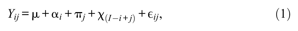
where $Y_{ij}$ is the observed value of the dependent variable in the $i$ th age group and $j$ th period, $μ$ represents the intercept, $α_{i}$ is the age effect for the $i$ th age group, $π_{j}$ is the period effect for the $j$ th period, $χ_{(I - i + j)}$ is the cohort effect for the $k$ th cohort $(k = I - i + j)$ , and $ϵ_{ij}$ is the residual term for the $ij$ th age-period-specific observation.

For concreteness, Table 2 shows the linear coding in a 4 by 5 age-period table. The linear coding for ages is 1 to 4 on the rows; the linear coding of periods is coded as 1 to 5 on the columns. Using this linear coding and ( $k = I - i + j)$ , we can generate the linear coding for cohorts; for example, the second age group in the second period is in cohort 4 (= 4 − 2 + 2), as is the first age group in the first period [4 (= 4 − 1 + 1)]. The linear effects of cohorts are linearly dependent on the linear effects of age and period. Thus, when the linear effects of age and period are in the model (when age and period are in the model), this controls for the linear effects of cohorts. Similar linear relationships apply to periods $(j = k - I + i)$ and to ages $(i = j - k + I)$ . Any two factors in the model account for the linear effect of the third factor.

Table 2.

Relationships between the Linear Effects of Ages, Periods, and Cohorts*

	Period 1 (1)	Period 2 (2)	Period 3 (3)	Period 4 (4)	Period 5 (5)
Age 1 (1)	4	5	6	7	8
Age 2 (2)	3	4	5	6	7
Age 3 (3)	2	3	4	5	6
Age 4 (4)	1	2	3	4	5

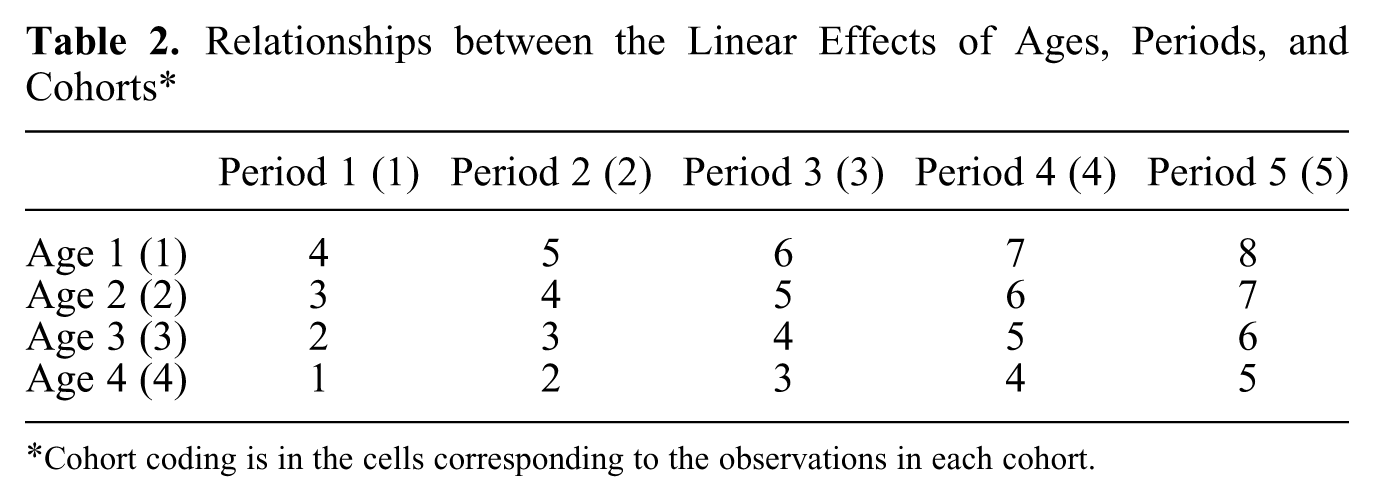
Cohort coding is in the cells corresponding to the observations in each cohort.

4. Relationships between the Linear Trends for Ages, Periods, and Cohorts

Although different constrained solutions can lead to very different estimates of the age, period, and cohort coefficients, the linear trends for ages, periods, and cohorts for different solutions are systematically related. Rodgers (1982:782) shows that the linear trends of the age-effects, period-effects, and cohort-effects are related to each other in the following straightforward manner (presented using my own notation):

t_{a}^{*} = t_{a} + k

t_{p}^{*} = t_{p} - k

t_{c}^{*} = t_{c} + k .

Interpreting the first equation, $t_{a}$ represents the linear trend in the age coefficients from an “original” constrained solution. If we calculate a different constrained solution and the linear trend in the age coefficients is $t_{a}^{*}$ and that trend is $k$ more than the linear trend for the original solution, then the trend for the new solution for periods will be $k$ less than the original trend for periods, and the trend in the cohort coefficients for the new solution will be $k$ greater than the linear trend for the cohort coefficients in the original solution. That is, different constrained solutions produce different trend estimates for the ages, periods, and cohorts, but the differences in the trends for ages, periods, and cohorts based on different solutions are systematically related. The relationships in equation 2 hold exactly when an APC model is based on a single just-identifying constraint. Equation 2 holds approximately when we drop one of the categorically coded factors from the model. Dropping one factor from the model results in more constraints than needed to identify the model. It constrains each of the categories of that factor to have a zero relationship with the dependent variable in the model and, because of this, a zero linear trend. This is why dropping the factor from the model does not exactly reproduce the pattern in equation 2 or produce fit statistics that are the same as when fixing one of the trends to zero.

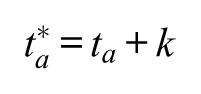
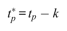
I focus in the following on two situations. Leaving one of the three factors out of the model is the situation most commonly found in the literature. The other is to constrain the trend of one of the factors to be zero, which is a just-identifying constraint and does follow equation 2 exactly. With categorical coding, the linear trends are similar using either strategy; but, as noted previously, they are not exactly the same. Intuitively, imagine that the trend of periods for the data-generating process is $k$ and $k$ is positive, but we constrain the slope for the period coefficients to be zero. This means that the expected value of the estimated trend under this constraint is not an unbiased estimate of the trend of the period parameters that generated the outcome data. It is too small by $k$ . Given equation 2, this also means that the trend for ages and for cohorts based on the data-generating process is overestimated by $k$ .

The relationships between the slopes of the three factors described in equation 2 provide insight into what happens when we drop one of the factors from the APC model.

The left-out factor’s effects are constrained to be zero, both its linear trend effects and the effects of its deviations from the linear trend.

When the model contains just two factors, those two factors take credit for their own linear trend effects, their effects that involve deviations from their linear trends, and they take credit for the linear trend effects of the third (left-out) factor.

Since the other two factors get credit for any linear trend effects in the data-generating process due to the left-out factor, this may make the two factors appear to be statistically significant even if their contribution to the data-generating process is not.

When the third factor is added to the two-factor model to determine whether it accounts for addition variance in the dependent variable, any variance due to its linear trend has already been “controlled for,” and the third factor will not get credit for any effects due to its linear trend.

With the test for incremental variance, only effects that are associated with the third factor’s deviations from its linear trend will be attributed to it.

Leaving the third factor out of the model based on its incremental fit not being statistically significant will too often eliminate a substantively important factor. This elimination affects the coefficient estimates of the two factors in the model.

This unique variance associated with the third factor is an estimable function (O’Brien 2014); it is the same no matter which just-identifying constraint is applied to the three-factor model. The increment in $R^{2}$ in this APCMC situation, however, is only a test of the nonlinear effects after any linear trend effect of the third factor has been removed.

5. Regression Procedures and Linear Trends for Ages, Periods, and Cohorts

The main purpose of this section is to provide a greater intuitive understanding of these relationships: Researchers typically have not (and will not) run these regressions while conducting their research (except for 1 below). I use cohort as an example of the “third” or left-out factor. The analogous procedures can be used with periods or ages as the left-out factor and with any GLM procedure.

Run an OLS regression with any single just-identifying constraint to calculate $R_{apc}^{2}$ . $R_{apc}^{2}$ is the proportion of the variance in the dependent variable accounted for by the age, period, and cohort factors. The individual age, period, and cohort effects differ depending on the constraint employed; however, $R_{apc}^{2}$ is the same for any just-identifying constraint.

Run a regression with just the age and period factors (categorically coded variables) and calculate $R_{ap}^{2}$ . To show that $R_{ap}^{2}$ captures these linear trend effects, regress the dependent variable on the age and period factors and with cohorts coded linearly from 1 to $K$ for the individual cohorts from earliest to most recent cohorts (as opposed to the categorical coding of cohorts). This model will require that you use one just-identifying constraint since the linear components for cohorts are included in the model. The result is $R_{ap (c_{L})}^{2}$ and $R_{ap}^{2} = R_{ap (c_{L})}^{2}$ (see again Table 1). The linear trends for the explicit $R_{ap (c_{L})}^{2}$ model (the model that codes the linear trend for cohorts and contains the age and period categorically coded variables) will differ depending on the constraint used to identify the model.

The difference between the $R^{2}$ for the full APC model and $R^{2}$ for the age and period factors $(R_{apc}^{2} - R_{ap}^{2})$ is due to the deviation of the cohort effects around the linear trend in the cohort effects. To show that this interpretation holds, we find the deviations of the cohort effects from their linear trend in a three-factor model. To calculate these deviations, run any $R_{apc}^{2}$ model with a single constraint. Calculate the trend in the cohort coefficients, then calculate the deviations in the estimated cohort coefficient from their predicted values based on this trend, then run a model with the age and period categorically coded variables and code each cohort with the deviations of the cohort coefficients from the linear trend in cohorts (these deviations are estimable functions). The result is $R_{ap (cohort deviations)}^{2} = R_{apc}^{2}$ . We can, of course, conduct such analyses with age or period as the third factor.

The F-test for the statistical significance of $R_{apc}^{2} - R_{ap}^{2}$ is often treated as a test of the importance of a third factor in the generation of the outcome variable. The standard F-test for the increment in variance accounted for does not test for the overall effects of cohorts in the process that generated the outcome data because it does not include any linear trend effects of cohorts. This incremental F-test for $R_{apc}^{2} - R_{ap}^{2}$ is a sufficient test for the statistical significance of the cohort factor since it indicates whether the cohort variation around its linear trend is statistically significant (without the additional variance in the dependent variable that might be accounted for by any linear trend in the cohorts). These deviations from the linear trend are estimable; they are the same no matter which just-identifying constraint is used to calculate $R_{apc}^{2}$ . This test can also be used to test the total effects of deviation from the linear trends for periods ( $R_{apc}^{2} - R_{ac}^{2}$ ) and for ages ( $R_{apc}^{2} - R_{pc}^{2}$ ). We assume throughout that the correctly specified model is the full APCMC model. Similar tests for GLM models, using likelihood chi-square tests, can be used with the same interpretational caveats.

There is a difference between leaving a factor out of the equation (then it is constrained to have no effect on the solution either from its linear trend or deviations around its linear trend) and constraining the linear trend to be zero. In the latter case, the linear trend effect is zero, but the deviations from the linear trend are allowed to account for variance in the dependent variable. In both cases, however, any linear effect in the factor is absorbed by the other two factors.

6. Discussion

One feature of the APC problem is nearly universally recognized: the impossibility of estimating a model with all three of these factors simultaneously in the model unless some sort of constraint is placed on the model to identify it. Placing a constraint on the model results in a specific set of estimates for the age, period, and cohort effects; a different constraint results in a different set of estimates. Only if the constraint is consistent with the parameters that generated the outcome variables will the solutions under the constraint be an unbiased estimate of those parameters. In fixed models, those constraints are explicit, and in mixed models (Bell and Jones 2014; O’Brien, Hudson, and Stockard 2008; Yang and Land 2006), the constraint is embedded in the model. The linear trends of ages, periods, and cohorts are linearly dependent, and this creates the APC identification problem, while the deviations around the linear trend of these factors are identified/estimable (Clayton and Schifflers 1987a, 1987b; Holford 1983; O’Brien 2014).

What is less well understood are the implications of the complete confounding (linear dependency) of the linear trends estimates of ages, periods, and cohorts on results that compare three-factor and two-factor models. For the categorically coded APC models that drop one of the factors from the model, any linear trend in the dropped out factor is absorbed by the other two factors. The two-factor model takes credit for any linear trend of the effects in the third factor. When the linear trend in the third factor is constrained to zero (rather than dropped from the model), the relationship between the effect of this constraint on the linear trend in the third factor and the linear trends in the other two factors is exact, as shown in equation 2. These insights explain specific shifts between the coefficients of the APCMC model when different factors are dropped from the model and show that the test for incremental variance should not be used as a criterion for dropping a factor from the model. The incremental fit test in the APCMC context is an atheoretical test that is likely to lead to a misspecified model.

What is the researcher to do? The following strategies are not a panacea, but they can provide valuable information about the age, period, and cohort effects.

Estimable functions do not depend on the constraint used to identify the APCMC model. Some examples of estimable functions are the second differences of age effects, period effects, and cohort effects: deviations of age effects from the linear trend in the age effects, deviations of period effects from linear trends in the period effects, and deviations of cohort effects from linear trends in the cohort effects and the variance accounted for by the three-factor model. Each of these estimable functions (and others) tells us something about the age, period, and cohort effects (O’Brien 2014).

Factor characteristic models can be used to estimate the effects of ages, periods, and cohorts. For example, we can categorically code ages and periods and code cohorts using a proxy variable such as the proportion of the cohort that was born out of wedlock or the relative size of the birth cohort. The effectiveness of this approach depends in part on how well the characteristics capture the effects of cohorts on the dependent variable (O’Brien 2000).

We can use a just-identifying constraint but should make sure the constraint is based on theory and/or substantive knowledge. The rationale is that if the theory and/or substantive knowledge are nearly correct and the constraint is based on these, then the constraint is more likely consistent with the data-generating parameters. If the constraint is approximately consistent with the data-generating parameters, it should provide an approximately unbiased estimate of those parameters. Using multiple approaches that reach similar conclusions will build confidence that the analysis may be getting at the data-generating parameters (O’Brien 2015a).

Footnotes

Notes

Author Biography

Robert M. O’Brien is a professor emeritus of sociology at the University of Oregon, where he taught for over 30 years. He specializes in criminology and quantitative methods and has published extensively in both areas. His interest in age-period-cohort models was kindled by a talk given by Bill Mason at the University of Oregon in the late 1980s. He published his first article using age-period-cohort models in Criminology in 1989. Recently he published a book titled Age-Period-Cohort Models: Approaches with Aggregate Data (Chapman and Hall, 2015). Other recent publications include “Dropping Highly Collinear Variables from a Model: Why It Typically Is Not a Good Idea” (Social Science Quarterly 2016), “Age-Period-Cohort Models and the Perpendicular Solution” (Epidemiologic Methods 2015), and “Estimable Functions of Age-Period-Cohort Models: A Unified Approach” (Quality and Quantity 2014).

References

Bell

Andrew

Jones

Kelvyn

. 2014. “Another ‘Futile Quest’? A Simulation Study of Yang and Land’s Hierarchical Age-period-cohort Model.”Demographic Research30:333–60.

Bell

Andrew

Jones

Kelvyn

. 2015. “Should Age-period-cohort Analyst Accept Innovation without Scrutiny? A Response to Reither, Masters, Yang, Powers, Zheng, and Land.”Social Science and Medicine128:331–33.

Clayton

Schifflers

1987a. “Models for Temporal Variation in Cancer Rates I: Age-period and Age-cohort Models.”Statistics in Medicine6:449–67.

Clayton

Schifflers

1987b. “Models for Temporal Variation in Cancer Rates II: Age-period-cohort Models.”Statistics in Medicine6:468–81.

Firebaugh

Glenn

. 1989. “Methods for Estimating Cohort Replacement Effects.” Pp. 243–62 in Sociological Methodology. Vol. 19, edited by Clogg

C. C.

Washington, DC: American Sociological Association.

Greenberg

David F.

Larkin

Nancy J.

1985. “Age-cohort Analysis of Arrest Rates.”Journal of Quantitative Criminology1:227–40.

Hall

Bronwyn H.

Mairesse

Jacques

Turner

Laure

. 2005. “Identifying Age, Cohort, and Period Effects in Scientific Research Productivity: Discussions and Illustration Using Simulated and Actual Data on French Physicists.”Working Paper No. 11739, National Bureau of Economic Research, Cambridge, MA.

Harding

David J.

Jencks

Christopher

. 2003. “Changing Attitudes toward Premarital Sex: Cohort, Period, and Aging Effects.”Public Opinion Research67:211–26.

Holford

Theodore R.

1983. “The Estimation of Age, Period, and Cohort Effects for Vital Rates.”Biometrics39:311–24.

10.

Luo

Liying

. 2013. “Assessing Validity and Application Scope of the Intrinsic Estimator Approach to the Age-period-cohort Problem.”Demography50:1945–67.

11.

Mason

William M.

Smith

Herbert L.

1985. “Age-period-cohort Analysis and the Study of Deaths from Pulmonary Tuberculosis.” Pp. 151–228 in Cohort Analysis in Social Research: Beyond the Identification Problem, edited by Mason

W. M.

Fienberg

S. E.

New York: Springer-Verlag.

12.

Mason

Karen O.

Mason

William M.

Winsborough

H. H.

Poole

W. Kenneth

. 1973. “Some Methodological Issues in Cohort Analysis of Archival Data.”American Sociological Review38:242–58.

13.

O’Brien

Robert M.

2000. “Age Period Cohort Characteristic Models.”Social Science Research29:123–39.

14.

O’Brien

Robert M.

2011a. “The Age-period-cohort Conundrum as Two Fundamental Problems.”Quality and Quantity45:1429–44.

15.

O’Brien

Robert M.

2014. “Estimable Functions in Age-period-cohort Models: A Unified Approach.”Quality and Quantity48:457–74.

16.

O’Brien

Robert M.

2015a. Age-period-cohort Models: Approaches and Analyses with Aggregate Data. New York: Chapman and Hall.

17.

O’Brien

Robert M.

Hudson

Kenneth

Stockard

Jean

. 2008. “A Mixed Model Estimation of Age, Period, and Cohort Effects.”Sociological Methods and Research36:402–28.

18.

Phillips

Julie A.

2014. “A Changing Epidemiology of Suicide? The Influence of Birth Cohorts on Suicide Rates in the United States.”Social Science and Medicine114:151–60.

19.

Rodgers

Willard L.

1982. “Estimable Functions of Age, Period, and Cohort Effects.”American Sociological Review47:774–87.

20.

Schaie

Klaus Warner

. 1965. “A General Model for the Study of Developmental Problems.”Psychological Bulletin64:92–107.

21.

Shahpar

Cyrus

Guohoa

. 1999. “Homicide Mortality in the United States, 1935–1994: Age, Period, and Cohort Effects.”American Journal of Epidemiology150:1213–22.

22.

Smith

Herbert L.

2004. “Response: Cohort Analysis Redux.” Pp. 111–19 in Sociological Methodology. Vol. 34, edited by Stolzenberg

R. M.

Oxford, UK: Basil Blackwell.

23.

Yang

Wenjiang J.

Land

Kenneth C.

2004. “A Methodological Comparison of Age-period-cohort Models: Intrinsic Estimator and Conventional Generalized Linear Models.” Pp. 75–110 in Sociological Methodology. Vol. 34, edited by Stolzenberg

R. M.

Oxford, UK: Basil Blackwell.

24.

Yang

Schulhofer-Wohl

Sam

Wenjiang J.

Land

Kenneth C.

2008. “The Intrinsic Estimator for Age-period-cohort Analysis: What It Is and How to Use It.”American Journal of Sociology113:1697–736.

25.

Yang

Land

Kenneth C.

2006. “A Mixed Models Approach to the Age-period-cohort Analysis of Repeated Cross-Section Surveys: Trends in Verbal Test Scores.” Pp. 75–97 in Sociological Methodology. Vol. 36, edited by Stolzenberg

R. M.

Oxford, UK: Basil Blackwell.

26.

Yang

Land

Kenneth C.

2013. Age-period-cohort Analysis: New Models, Methods, and Empirical Applications. New York: Chapman and Hall.