Decomposition Analysis of Segregation

Abstract

Although substantive studies on segregation, such as residential or school segregation by race and occupational segregation by gender, are many in sociology, the analytical methodology is almost exclusively focused on measurement issues. The author introduces a set of two statistical models for the decomposition analysis of segregation. These models can be regarded as a tool to analyze whether one dimension of racial or gender inequality is related to another dimension of inequality, because they can assess, for example, the extent to which gender differences in human capital are related to gender segregation in occupation. One of the new models is a simple extension of the DiNardo-Fortin-Lemieux decomposition method of inequality, which implicitly assumes a supply-driven determination of positional status attainment, and another model modifies it to incorporate demand-based macrosocial size constraints on positional status attainment, but both models rely on Rubin’s conception of modeling counterfactual outcomes and inverse-probability-of-treatment weighting on the basis of propensity score. An application focuses on gender segregation in occupation in Japan and leads to a paradoxical result: equalizing human capital and labor supply characteristics between men and women increases, rather than decreases, gender segregation in occupation. Although the underlying behavioral mechanism for gender differences in occupational choice remains to be investigated, the analysis clarifies at least demographically why segregation increases under the counterfactual situation.

Keywords

segregation analysis index of dissimilarity decomposition propensity score matching model DiNardo-Fortin-Lemieux method

1. Introduction

Segregation analysis is a central topic in sociological research. Substantive research on segregation includes numerous studies of residential segregation and school segregation by race and ethnicity and occupational segregation by gender. In this article I introduce two alternative, mutually complementary models for the decomposition of the extent of segregation into “explained” and “unexplained” components. This article is concerned in general with the methodology of estimating the unique effect of the group variable X on segregation when the covariates of the group variable also affect segregation, and therefore the observed effect of X on segregation is confounded by the effect of the association of X with covariates on segregation. The “explained” component of the segregation represents the extent of segregation that is explained by differences in the covariate distribution between the group with X = 1 and the group with X = 0, and the “unexplained” component represents the remaining extent of segregation. Substantive examples may include (1) a case in which race and household income affect the choice of residential district, and we are concerned with the hypothetical extent of residential racial segregation after eliminating the indirect combined effect of (a) the association between race and household income and (b) the effects of household income on the choice of residential district; and (2) a case in which gender is associated with the characteristics of educational attainment, such as years of education and college majors, and both gender and educational characteristics affect the choice of occupation, and we are concerned with the hypothetical extent of gender segregation in occupation after eliminating the indirect combined effect of (a) the association of gender and educational characteristics and (b) the effects of education on the choice of occupation. In both cases, the models described in this article eliminate the indirect effect by removing factor (a) by attaining statistical independence between the group variable and covariates.

The two models introduced here both rely on propensity-score weighting (Robins 1998; Rubin 1985), employed in Rubin’s causal model (RCM). One of them is a simple extension of the DiNardo-Fortin-Lemieux (DFL) method (DiNardo, Fortin, and Lemieux 1996) for decomposition analysis, extended for a polytomous outcome variable and applied to decompose the index of dissimilarity (ID). The other model, which is newly introduced in this article, is what I refer to as the matching model.¹ Like the RCM, the DFL method makes the stable unit treatment assignment (SUTVA) assumption, which leads to the fact that the distribution of outcomes, such as occupational distribution in the analysis of gender segregation in occupation and residential distribution in the analysis of residential racial segregation, depends only on the supply-side characteristics, namely, characteristics of people who attain those occupational or residential positions. As a result, when we consider a counterfactual situation, such as would be realized if women came to have the same human capital characteristics as men, occupational distribution changes according to changes in the supply-side labor characteristics. On the other hand, the matching model assumes that the outcome distribution is determined only by the demand-side characteristics, so that job vacancies or residential vacancies will be filled to the extent to which demand for the occupants of those positions exists, and therefore, changes in the supply-side characteristics conceived under a counterfactual situation do not affect the outcome distribution of positions but alter only the matching between people and positions. The matching model does not satisfy the SUTVA assumption because it introduces macrosocial constraints on the outcome distribution (Yamaguchi 2011). However, as shown in this article, the matching model retains all other characteristics of the DFL method.

If in reality the attainment of social positions will be neither completely supply driven nor completely demand driven but will depend on both the supply and the demand for those positions, the results from both the model based on the DFL method and the matching model identify a range of outcomes in which the counterfactual outcome will be realized.

Not unlike the DFL method, the two models for the decomposition of segregation are not methods for causal analysis because I do not intend to claim that the covariates included exhaust all determinants of the outcome other than the group variable X, which means, therefore, that omitted-variable bias certainly exists. In addition, the issue of controlling endogenous intervening variables also exists for the DFL method in making a causal inference (Yamaguchi 2015). Instead, the purpose of the two models introduced in this article is to separate the observed extent of segregation into a component explained by the association of the group variable X with a given set of covariates V that also affect the outcome and the remaining unexplained component, without claiming that the unexplained effect is a causal effect.

Methodological interest in segregation analysis has been centered on which measure has the most desirable characteristics (e.g., Blackburn and Marsh 1991; Lieberson 1976; Reardon and Firebaugh 2002; Reardon and O’Sullivan 2004; Winship 1977), given the fact that the ID, which is still a representative measure of segregation, may be better modified to reflect certain additional characteristics such as distance among the units of segregation for measuring residential segregation. This is an important methodological issue, but it is largely independent of the topic of this article, because the decomposition methods introduced here can be combined with different segregation indices of the researcher’s choice as long as they are modifications of the ID based on the measurement of differences between groups in the categorical distribution of segregation units. Charles and Grusky (1995, 2004) introduced log-linear and log-multiplicative models for segregation focusing on gender segregation in occupation. Their method measures segregation on the basis of characteristics of the odds ratio and requires a distinct methodological approach to the decomposition of segregation. In this article, however, I focus on the decomposition of segregation based on the ID. Below, I introduce the decomposition of the ID by an extension of the DFL method and by the matching model and apply them to an analysis of gender segregation of occupation in Japan.

2. Methods

2.1. A Brief Review of the DFL Method

Unlike the Blinder-Oaxaca decomposition method (Blinder 1973; Oaxaca 1973), which relies on a pair of regression equations for the outcome, the DFL method does not assume any parametric model for the outcome. As Barsky et al. (2002) pointed out, a major limitation of the Blinder-Oaxaca method is that it requires a linear relationship between the dependent variable and its covariates. On the other hand, the DFL method, which does not assume such a relationship, is considered (Fortin, Lemieux, and Firpo 2011) to be a method that generates a more robust estimate for decomposition than the methods that rely on regression models.

The pair of equations assumed for men and women can be expressed in the DFL method as $y^{M} = ϕ (V^{M}, θ^{M}) + ε$ for men and $y^{W} = ϕ (V^{W}, θ^{W}) + ε$ for women, where $ϕ$ is an unspecified function, $V^{M}$ and $V^{W}$ are covariates of the outcome, and $θ^{M}$ and $θ^{W}$ are parameters that indicate the covariate effects of the outcome, for men and women, respectively. Under the assumed independence of the error term from the covariates, we may obtain the following decomposition:

{\bar{y}}^{W} - {\bar{y}}^{M} = [\bar{ϕ} (V^{W}, θ^{W}) - \bar{ϕ} (V^{M}, θ^{W}))] + [\bar{ϕ} (V^{M}, θ^{W}) - \bar{ϕ} (V^{M}, θ^{M}))] .

The first component—the “explained” component—of equation (1) reflects inequality in the mean of Y that would be eliminated if women had men’s covariate distribution, and the second component—the “unexplained” component—reflects inequality that would remain because women having the same covariate distribution as men are treated differently in the society. Because the estimates of $\bar{ϕ} (V^{M}, θ^{M})$ and $\bar{ϕ} (V^{W}, θ^{W})$ are simply sample means, we need only an estimate of $\bar{ϕ} (V^{M}, θ^{W})$ , which can be obtained from the following equation for the gender dummy variable X that takes a value of 0 for men and 1 for women:

\begin{matrix} \bar{ϕ} (V^{M}, θ^{W}) \equiv \int_{v} ϕ (v, θ^{W}) p (v | X = 0) d v = \int_{v} E (Y^{W} | v) p (v | X = 0) d v \\ = \int_{v} ω (v) E (Y^{W} | v) p (v | X = 1) d v = E_{ω} (Y^{W}), \end{matrix}

where $p (v | X)$ indicates the conditional probability density of V, and $E_{ω}$ indicates the weighted mean with weights:

ω (v) \equiv \frac{p (v | X = 0)}{p (v | X = 1)} = \frac{p (X = 0 | v) p (v) / p (X = 0)}{p (X = 1 | v) p (v) / p (X = 1)} = \frac{p (X = 1) p (X = 0 | v)}{p (X = 0) p (X = 1 | v)} .

Unlike the Blinder-Oaxaca method, the DFL method can be applied to the decomposition of difference in proportion, as in the decomposition analysis of gender difference in the proportion of managers, because it does not assume any outcome regression model. The method introduced in this article takes this advantage of the DFL method further by extending its application to the case of a polytomous dependent variable.

2.2. The DFL Model, Where the Marginal Distribution of Outcomes Is Endogenously Determined under Counterfactual Situations

I introduce below a decomposition method, which I call the DFL model, for the ID, using an example of gender segregation in occupation, by extending the DFL method. We are interested in the decomposition of $P_{j}^{M} - P_{j}^{W}$ , for a set of occupations with j = 1, . . ., J, where $P_{j}^{M}$ is the proportion, among men who have jobs, of those in the jth occupation, and $P_{j}^{W}$ is the proportion, among women who have jobs, of those in the jth occupation, into the component attributable to gender differences in covariates V, such as educational attainment, age, marital status, and hours of work, and the unexplained component. If this decomposition is attained, then we can decompose the ID, defined as $(1 / 2) \sum_{j} | P_{j}^{M} - P_{j}^{W} |$ , into the unexplained component, defined as $(1 / 2) \sum_{j} | {(P_{j}^{M} - P_{j}^{W})}_{unexplained} |$ , where $(P_{j}^{M} - P_{j}^{W})_{unexplained}$ is the unexplained gender difference in the proportion estimated by the method described below, and the explained component, which is the difference between the observed ID value and the unexplained ID value.

Generally, we assume that the marginal distribution of the group variable X, such as gender or race, is fixed under any counterfactual situation. On the other hand, the marginal distribution of covariates V summed over the states of X depends on a particular counterfactual situation that we assume but is assumed nonetheless to be exogenously determined independently of the association between X and V. First, in this section we assume further a model that implicitly makes the SUTVA assumption (Morgan and Winship 2007) for potential outcomes. With this assumption, we can define the saturated linear probability model for the outcome with categorical covariates for the probability of having outcome j as a function of the covariates of individuals and outcome-specific parameters as follows:

\Pr (Y_{i} = j) \equiv P_{ij} = α_{j} (v_{i}; θ_{0 j}) + β_{j} (v_{i}; θ_{1 j}) X_{i}, for j = 1, \dots, J - 1,

where Y_i is a categorical outcome variable for person i; $P_{ij}$ is the probability for person i with covariates $v_{i}$ , where $v_{i}$ is the value of V observed for person i, to attain the jth occupation; $α_{j} (v_{i}; θ_{0 j})$ represents the “main effects” of covariates V with the outcome-specific parameters $θ_{0 j}$ ; $X_{i}$ is a gender dummy variable that takes a value of 0 for women and a value of 1 for men for person i; and $β_{j} (v_{i}; θ_{1 j}) X_{i}$ represents the heterogeneous effects of gender, with heterogeneity varying with covariates $V$ , on the outcome with the outcome-specific parameters $θ_{1 j}$ . Note that although it may be thought that a linear probability model will generate inconsistent parameter estimates, we assume here a saturated model with categorical covariates where the estimated probabilities are equal to sample proportions for each combined state of covariates, and for any saturated model no inconsistency issue exists. Note also that the marginal distribution of the jth occupation is determined by the effects of X and V on P_ij characterized by parameters $α_{j} (v_{i}; θ_{0 j})$ and $β_{j} (v_{i}; θ_{1 j})$ . In other words, the size of each occupation here is implicitly assumed to be endogenously determined by supply-side characteristics of the labor market, that is, the joint distribution of $(X, V)$ for a given set of parameters ${θ_{0 j}, θ_{1 j}}$ .

From equation (1), we obtain $\Pr (Y = j | X = 0) \equiv P_{j}^{W} = E (α_{j} (v) | X = 0)$ and $\Pr (Y = j | X = 1) \equiv P_{j}^{M} = E (α_{j} (v) | X = 1) + E (β_{j} (v) | X = 1)$ , where $P_{j}^{W}$ and $P_{j}^{M}$ are the means of $P_{ij}$ for men and women, respectively, with each outcome j, and those means for men and women are equal to their sample proportions for saturated models. It follows that

P_{j}^{M} - P_{j}^{W} = {E (α_{j} (v) | X = 1) - E (α_{j} (v) | X = 0)} + E (β_{j} (v) | X = 1) .

This equation indicates that the observed gender difference in the proportion of having the jth job is the sum of the gender difference in the main average covariate effects and the average gender effect among men.

Suppose that we realize a counterfactual situation in sample data in which the covariate distribution becomes statistically independent of X by multiplying weights ω(v) to sample observations. Then, because $E_{ω} (α_{j} (v) | X = 1) = E_{ω} (α_{j} (v) | X = 0)$ holds, where $E_{ω}$ indicates the weighted mean, under $V ⊥ X$ , we obtain

E_{ω} (Y = j | X = 1) - E_{ω} (Y = j | X = 0) = E_{ω} (β_{j} (v) | X = 1) = E_{ω} (β_{j} (v)),

and, therefore, $E_{ω} (Y = j | X = 1) - E_{ω} (Y_{j} = j | X = 0)$ reflects the weighted average of the gender effect. Note that the conditioning by X = 1 for $β$ can be omitted because the weighted average of $β$ depends only on the weighted distribution of V, which is made equal between X = 1 and X = 0.

Regarding the distribution of V, which is to be made equal between the group with X = 1 and the group with X = 0 for the weighted data, we can consider three meaningful alternative situations:

a counterfactual situation in which both men and women come to have the average covariate distribution $P (v)$ ,

a counterfactual situation in which women come to have men’s covariate distribution $P (v | X = 1)$ , and

a counterfactual situation in which men come to have women’s covariate distribution $P (v | X = 0)$ .

As shown below, these three counterfactual situations are similar to those considered for the estimation of the average treatment effect, the average treatment effect for the treated, and the average treatment effect for the untreated (Morgan and Winship 2007), although we do not make a causal interpretation of those “treatment effects,” for reasons explained above. In addition, the distinction between X = 1 and X = 0 is not a distinction between the treatment group and the control group here, and we will therefore refer to the effect of X under the three alternative situations for the covariate distribution as the average group effect (AGE), the AGE for group 1 (AGE1), and the AGE for group 0 (AGE0).

As initially shown by Rubin (1985; see also Robins 1998, and described by Morgan and Winship 2007), the AGE can be estimated by using the following sets of inverse-probability-of-treatment (IPT) weights:

ω_{1} (v) = \frac{P (v)}{P (v | X = 1)} = \frac{P (X = 1)}{P (X = 1 | v)}

for men, for whom X = 1 holds, and

ω_{0} (v) = \frac{P (v)}{P (v | X = 0)} = \frac{P (X = 0)}{P (X = 0 | v)}

for women, for whom X = 0 holds.

By those weightings, the covariate distributions for both men and women become nearly equal when the propensity score, $P (X = 1 | v)$ , is adequately estimated. Note that when $P (X = 1 | v)$ can be estimated nonparametrically because we have observations for both X = 1 and X = 0 for each combined state of the covariates, the conversion of $P (v | X = 1)$ and $P (v | X = 0)$ to $P (v)$ by using their nonparametric estimates for the IPT weighting will be perfect. For a parametric estimate of $P (v | x)$ , we expect that the weighting, when the propensity score is adequately estimated, will attain statistical independence between X and V. However, we need to diagnose this expected property of the IPT weights, because this property may not be attained either when we have a model of $P (v | x)$ that does not fit the data or when observations that lie outside the “common area of support” for the propensity score generate nonnegligible bias in attaining statistical independence between X and V. This issue will be addressed in the application.

It is also noteworthy that in order to retain the marginal distribution of X, weights $ω_{1} (v)$ and $ω_{0} (v)$ need to be replaced by the adjusted weights $ω_{1} * (v)$ and $ω_{0} * (v)$ for the ratio estimation so that the sum of the weights becomes equal to the sample size in each group of X:

ω_{1} * (v_{i}) = \frac{N_{1} ω_{1} (v_{i})}{\sum_{k = 1 | X = 1}^{N_{1}} ω_{1} (v_{k})} and ω_{0} * (v_{i}) = \frac{N_{0} ω_{0} (v_{i})}{\sum_{k = 1 | X = 0}^{N_{0}} ω_{0} (v_{k})},

where N₁ and N₀ indicate the number of sample observations with X = 1 and X = 0, respectively. The unexplained difference in the proportion in unit j between men and women is then given as

E_{ω_{1} *} (Y = j | X = 1) - E_{ω_{0} *} (Y = j | X = 0),

where $E_{ω_{1} *} (Y = j | x)$ indicates the weighted average probability of being in unit j with adjusted weights of equation (9). This is the estimate for the AGE.

When we consider an alternative counterfactual situation in which women have the covariate distribution of men, the weights for women and their adjustment for the ratio estimation are given, as in equation (3), as

ω_{01} (v) \equiv \frac{P (v | X = 1)}{P (v | X = 0)} = \frac{P (X = 0) P (X = 1 | v)}{P (X = 1) P (X = 0 | v)}, and

ω_{01} * (v_{i}) = \frac{N_{0} ω_{01} (v_{i})}{\sum_{k = 1 | X = 0}^{N_{0}} ω_{01} (v_{k})} .

The unexplained difference in the proportion in unit j between men and women is then given as

E (Y = j | X = 1) - E_{ω_{01} *} (Y = j | X = 0) .

This is the estimate for the AGE1. Similarly, the estimate for the AGE0 is obtained for the difference in the proportion in the counterfactual situation in which men have the covariate distribution of women by switching men and women in equations (11) through (13).

2.3. The Matching Model, Where the Marginal Distribution of Outcomes Is Exogenously Determined under Counterfactual Situations

In the model introduced in Section 2.2, it is implicitly assumed that the size of the outcome categories, such as the proportion of people in each occupation, is endogenously determined and can change depending on supply-side characteristics, characterized by the joint distribution of the group variable X and covariates V. Let us demonstrate this first by using a simplified case of dichotomous occupational distinction, such as managers and other employees, and dichotomized covariate states, which we denote by V. We assume that the probability distribution of the cross-classification of gender and covariates is as given in Table 1.

Table 1.

Cross-classified Proportions of Gender and Covariates

	Men: X = 1	Women: X = 0
V = 1	Q	S
V = 0	R	T

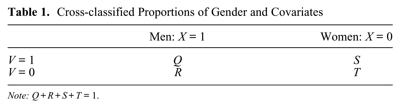
Note: Q+R+S+T = 1.

The saturated linear probability of being a manager at the individual level, its average, and the difference in the proportion of managers between men and women are then given, respectively, as

\begin{matrix} P_{i} = α + β_{1} X_{i} + β_{2} V_{i} + β_{3} X_{i} V_{i}, \end{matrix}

\begin{matrix} \bar{P} = α + (β_{1} + β_{2} + β_{3}) Q + β_{1} R + β_{2} S \\ = α + β_{1} (Q + R) + β_{2} (Q + S) + β_{3} Q, and \end{matrix}

\begin{matrix} {\bar{P}}^{M} - {\bar{P}}^{W} = \frac{α (Q + R) + (β_{1} + β_{2} + β_{3}) Q + β_{1} R}{Q + R} - \frac{α (S + T) + β_{2} S}{S + T} \\ = β_{1} + β_{3} (\frac{Q}{Q + R}) + β_{2} (\frac{Q}{Q + R} - \frac{S}{S + T}) . \end{matrix}

We retain the proportions of men and women, Q+R and S+T, for any of the counterfactual situations considered here. The proportion of people with V = 1, Q+S, is retained only for the AGE but not for the AGE for group 0 (AGE0) or that for group 1 (AGE1). Equation (15) then shows that neither the AGE0 nor the AGE1 preserves the average proportion of managers under each counterfactual situation, because Q+S changes for each counterfactual situation. On the other hand, the AGE preserves the average proportion of managers if the effects of X and V are additive, but this does not hold when an interaction effect of X and V exists, because $\bar{P}$ then changes with Q, which does not remain constant under any of the three counterfactual situations. This holds in the general case in which the covariate V has many more categories, because equation (15) holds for the dichotomous distinction between each category and the rest of the categories combined. Equation (16) simply demonstrates the fact that the confounding covariate effect will be eliminated when X becomes statistically independent of V and, therefore, Q/(Q+R) = S/(S+T) holds.

The model of equation (4) assumes that the sizes of the outcome categories vary freely with the supply-side characteristics of labor under the counterfactual situation. This assumption may be unrealistic, however. In the case of residential segregation, change in the association between race and household income may not change the number of people living in each residential district. Similarly, for the case of occupational segregation by gender, change in the association between gender and education may change only the matching between occupation and people, not the number of people in each occupation. Below, we consider the matching model, an alternative model in which the sizes of outcome categories are invariant under a counterfactual situation in which the group variable and covariates become independent. In the analysis of occupational segregation, this leads to a model in which demand by employers, rather than supply-side characteristics, determines the number of occupants of each occupation.

For the matching model, we need to modify the model of equation (4) as follows:

\Pr (Y_{i} = j) \equiv P_{ij} = ϕ_{j} (V, x) {α_{j} (v_{i}; θ_{0 j}) + β_{j} (v_{i}; θ_{1 j}) X_{i}}, for j = 1, \dots, J - 1,

where $ϕ_{j}$ is an outcome category–specific parameter and is a function of the joint distribution of $V \equiv {v_{i}}$ and $x = {x_{i}}$ . Parameters ${ϕ_{j}}$ are constant and take a value of 1 for observed data and take values under a given counterfactual situation to make the average probability of attaining each outcome status remain the same as the proportion of people that is observed in the unit. Note that because parameters { $ϕ_{j}$ } depend on the macrosocial joint distribution of X and V, the matching model does not satisfy the SUTVA assumption.

The model of equation (17) might be thought to be underidentified, because we assume that $α_{j} (v_{i}; θ_{0 j}) + β_{j} (v_{i}; θ_{1 j}) X_{i}$ is the saturated model for observed data with zero degrees of freedom. In fact, equation (17), as well as equation (4), is a model for predicting outcomes for a counterfactual situation. Hence, if conditions to be met for a particular counterfactual situation are given, it can be identified. For the model of equation (17), we assume that a counterfactual situation satisfies the following five conditions, four of which, (a) through (d), are shared by the DFL model, and one of which, condition (e), is unique to the matching model:

Parameters $α_{j} (v_{i}; θ_{0 j})$ and $β_{j} (v_{i}; θ_{1 j})$ are fixed for each given v_i.

The marginal distribution of the group variable X is fixed and is equal to the observed distribution.

The marginal distribution of the covariates is exogenously imposed on one of the following depending on whether we estimate the AGE, AGE0, or AGE1, that is, $P (v)$ , $P (v | x = 1), or P (v | x = 0)$ .

The group variable and covariates become statistically independent.

The marginal distribution of the outcome categories $\Pr (Y = j)$ is fixed and is equal to the observed distribution, and this is attained by the adjustment of parameter $ϕ_{j}$ for each counterfactual joint distribution of X and V.

Given the model of equation (17), we obtain the following equalities:

E (Y = j | X = 0) \equiv P_{j}^{W} = ϕ_{j} E (α_{j} (v) | X = 0), and

E (Y = j | X = 1) \equiv P_{j}^{M} = ϕ_{j} E (α_{j} (v) | X = 1) + ϕ_{j} E (β_{j} (v) | X = 1) .

Hence, under the counterfactual situation in which X becomes independent of covariates V by the use of weights $ω_{M} (v)$ , which differ from the weights for the DFL method (hereafter, “the DFL weights”) as explained below, $E_{ω_{M}} (α_{j} (v) | X = 1) = E_{ω_{M}} (α_{j} (v) | X = 0)$ holds.

Hence, we obtain

E_{ω_{M}} (Y = j | X = 1) - E_{ω_{M}} (Y = j | X = 0) = ϕ_{j} E_{ω_{M}} (β_{j} (v)) .

The remaining issue is how to obtain estimates of the set of ${ϕ_{j}}$ that satisfies conditions (a) through (e) above. Note that $ϕ_{j}$ is not simply equal to $E (Y = j) / E_{ω_{DFL}} (Y = j)$ , where $ω_{DFL}$ denotes the DFL weights, because the adjustment by $E (Y = j) / E_{ω_{DFL}} (Y = j)$ does not preserve the statistical independence between X and V.

Let us denote by $f (x, y, v)$ the observed joint frequency distribution and denote by $F_{1} (x, y, v)$ the initial estimate of the counterfactual joint frequency distribution by the DFL method. When the propensity score is estimated nonparametrically, $F_{1} (x, y, v)$ is an estimate that satisfies conditions (a) through (d) but may not satisfy condition (e). When the propensity score is estimated parametrically using logit or probit regression, we need to diagnose and make sure that condition (d), regarding statistical independence between X and V, is satisfied in the sample with the DFL weights. When $F_{1} (x, y, v)$ satisfies conditions (a) through (d), we then need to estimate the expected joint distribution $F (x, y, v)$ that satisfies both $F (x, +, v) = F_{1} (x, +, v)$ , in consequence of which $F (x, y, v)$ will satisfy conditions (b) through (d), and $F (+, y, +) = f (+, y, +)$ , in consequence of which $F (x, y, v)$ will satisfy condition (e). Here the plus sign indicates the sum across categories. Condition (a) is also satisfied by the use of multiplicative iterative adjustments of frequencies described below. In the case of the AGE that preserves the marginal distribution of covariates, the above-described model is in fact a special case of the marginal model (Bergsma and Rudas 2002), for which $F (x, +, v) = f (x, +, +) f (+, +, v)$ and $F (+, y, +) = f (+, y, +)$ hold.

It might be objected that although the marginal model is a log-linear model, we have a modification of the additive model here. Note, however, that the additive component is saturated for the observed data, and we fix it for any counterfactual situation and, therefore, do not need to estimate those parameters. On the other hand, the model of equation (17) is multiplicative, or log-linear, regarding the set of $ϕ$ parameters that we need to estimate, and we can therefore employ the method of model fitting and parameter estimation for the log-linear model.

We can use the iterative proportional adjustment, across rounds of iterative estimation starting with t = 1, to obtain the final estimate of $F * (x, y, v)$ that should be attained when the adjustments lead to a convergence:

Calculate $F_{2 t - 1} (+, y, +) = \sum_{x} \sum_{v} F_{2 t - 1} (x, y, v)$ .

Calculate $F_{2 t} (x, y, v) = F_{2 t - 1} (x, y, v) \frac{f (+, y, +)}{F_{2 t - 1} (+, y, +)}$ .

Calculate $F_{2 t} (x, +, v) = \sum_{y} F_{2 t} (x, y, v)$ .

For the case in which $F_{1} (x, +, v)$ > 0, calculate $F_{2 t + 1} (x, y, v) = F_{2 t} (x, y, v) \frac{F_{1} (x, +, v)}{F_{2 t} (x, +, v)}$ .

The ratio of the final estimate to the initial estimate can then be expressed as $F * (v, j, x) / F_{1} (v, j, x) = {\hat{ϕ}}_{j} φ (v, x)$ , where ${\hat{ϕ}}_{j}$ is the product of iterative adjustments made in step (2) of the iterative procedure and is the estimate of parameter $ϕ_{j}$ in equation (17), and $φ (v, x)$ is the product of iterative adjustments made in step (4) of the iterative procedure and the modifier of the DFL weights. Note that weights $ω_{DFL} (v, x) φ (v, x)$ preserve the statistical independence between X and V in $F * (x, +, v)$ because $F * (x, +, v) = F_{1} (x, +, v)$ , and they are the weights for the matching model, that is, $ω_{M} (v, x) = ω_{DFL} (v, x) φ (v, x)$ .

3. Application

3.1. Data and the Main Descriptive Characteristics of Occupational Segregation

As an illustrative analysis, I focus on gender segregation in occupation among employees aged 23 to 59 years in Japan on the basis of the 2005 Social Stratification and Mobility (SSM) survey, which collects data from a national representative sample of men and women aged 20 to 69 years. Those under age 23 and those over 60 are excluded from this analysis to reduce selection bias caused by gender-specific college attendance rates and gender-specific retirement processes. This survey is chosen for this analysis because of its detailed collection of information on occupation and education, including high school types and college majors for the latter.

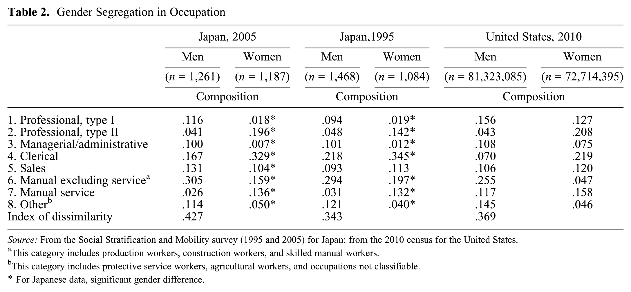
Gender segregation in occupation in Japan exists for several reasons. Among nonmanual workers, women are overrepresented in clerical occupations and the “middle- and lower-status” human service professions, which I will refer to as “type II professionals,” distinguished from other professionals, which I will refer to as “type I professionals.” By human services, I mean occupations related to medicine, education, human care, and welfare. By the term middle and lower status, I imply the exclusion of high-status professionals in medicine and education, namely, physicians, surgeons, and dentists in medicine and post–secondary school teachers in education. Among manual workers, women are overrepresented in service work. Table 2 presents the composition of occupation by gender and the ID, and for comparison, it also presents numbers for the 1995 SSM survey for Japan and numbers for the United States on the basis of the 2010 population census. The results in Japan are weighted by sampling weights provided by the researchers who conducted the survey. Information on the correspondence of the eight occupational categories to the 2010 U.S. census classification codes for occupations is available from the author on request.

Table 2.

Gender Segregation in Occupation

	Japan, 2005		Japan,1995		United States, 2010
	Men	Women	Men	Women	Men	Women
	(n = 1,261)	(n = 1,187)	(n = 1,468)	(n = 1,084)	(n = 81,323,085)	(n = 72,714,395)
	Composition		Composition		Composition
1. Professional, type I	.116	.018*	.094	.019*	.156	.127
2. Professional, type II	.041	.196*	.048	.142*	.043	.208
3. Managerial/administrative	.100	.007*	.101	.012*	.108	.075
4. Clerical	.167	.329*	.218	.345*	.070	.219
5. Sales	.131	.104*	.093	.113	.106	.120
6. Manual excluding service^a	.305	.159*	.294	.197*	.255	.047
7. Manual service	.026	.136*	.031	.132*	.117	.158
8. Other^b	.114	.050*	.121	.040*	.145	.046
Index of dissimilarity	.427		.343		.369

Source: From the Social Stratification and Mobility survey (1995 and 2005) for Japan; from the 2010 census for the United States.

This category includes production workers, construction workers, and skilled manual workers.

This category includes protective service workers, agricultural workers, and occupations not classifiable.

For Japanese data, significant gender difference.

Table 2 also shows that a great deal of gender segregation in occupation exists in both Japan and the United States, and the extent is greater in Japan than in the United States. However, a more important fact is that although there are commonalities and differences between the two countries in the pattern of gender segregation in occupation, those differences always indicate greater disadvantages of women in Japan than in the United States, as explained below.

There are commonalities between Japan and the United States showing that women are significantly overrepresented in type II professional work and clerical work. The differences are that in Japan women are strongly underrepresented in type I professional and managerial positions and strongly overrepresented in service work. Although gender differences exist for those occupations in the United States as well, the extent of gender difference is much smaller. Those differences between Japan and the United States indicate the relative disadvantages of women in Japan in comparison with women in the United States. On the other hand, men are much more overrepresented in nonservice manual occupations in the United States than in Japan. This difference between Japan and the United States indicates a relative disadvantage of men in the United States in comparison with men in Japan, given that average earnings are lower for manual workers than for nonmanual workers. Hence, all differences between Japan and the United States in gender segregation in occupation indicate stronger disadvantages of women in Japan than in the United States.

A comparison of the 1995 and 2005 results in Japan also shows that the extent of gender segregation in occupation increased over time in Japan. This change occurred because both the extent of women’s overrepresentation in type II professional occupations and the extent of women’s underrepresentation in nonservice manual work became greater in 2005 than in 1995 despite an increase in gender equality of educational attainment over the decade.

Table 3 also shows that Japanese women are disadvantaged in other respects, that is, in postsecondary education and in employment status. Women are severely underrepresented in receiving a four-year college education in Japan and are overrepresented in irregular employment. The overrepresentation of women in irregular employment comes mainly from a combination of the facts that the majority of women work either part-time or full-time without overtime work and that the majority of men work full-time with overtime work, as shown in Table 3, and there is a very strong association between hours of work and employment status in Japan, such that among those who work less than 35 hr per week, in which women are heavily overrepresented, 91.1 percent are irregularly employed, among those who work 35 to 40 hr per week, in which women are somewhat overrepresented, 24.5 percent are irregularly employed, and among those who work 41 hr or more per week, in which women are strongly underrepresented, 8.7 percent are irregularly employed. Gender inequality in educational attainment also varies strongly with age. I will examine whether gender inequality in education, age, and labor supply partially explains gender segregation in occupation.

Table 3.

Gender Inequality in Education and Employment Status

	Men	Women
	(n = 1,261)	(n = 1,187)
	Composition
1. Proportion who are 4-year college graduates	.377	.148*
2. Proportion who are irregular workers	.078	.520*
3. Composition by hours of work per week
<35 hr	.024	.333*
35–40 hr	.323	.398*
41–49 hr	.235	.161*
50–59 hr	.192	.062*
≥60 hr	.211	.032*
Missing	.015	.014
Total	1.000	1.000

Source: From the 2005 Social Stratification and Mobility survey.

Significant gender difference.

3.2. Decomposition Analysis of Occupational Segregation by Gender

Table 4 presents the main results of the decomposition analysis of occupational segregation on the basis of the data from the 2005 SSM survey for the counterfactual situation in which women’s covariate distributions become equal to men’s (AGE1). They are based on the use of data weighted by sampling weights. Model 1 includes age and education, including the category-by-category interaction effects of education and age, which are found to be significant, as covariates. Model 2 adds to model 1 marital status (married vs. single) and number of children (0, 1, 2, and ≥3) as covariates,² including the category-by-category interaction effects of age and marital status, and the category-by-category interaction effects of marital status and number of children, which are also found to be significant. Model 3 adds to model 2 the six-category distinction of hours of work per week (<35 hr, 35–40 hr, 41–49 hr, 50–59 hr, ≥60 hr, and “missing”) and the two interaction effects that are found to be significant in predicting propensity score and are necessary to attain statistical independence between gender and the hours of work in the inverse-probability-weighted sample. Those interaction effects are (1) the interaction effect of being married and working less than 35 hr per week and (2) the interaction effect of being a college graduate and working 60 hr or more per week, both of which imply that women are more likely to have those combinations beyond the additive effects of the two variables.

Table 4.

Main Results for the Decomposition of Segregation

	Occupational Segregation: Sample ID = .427
	DFL	Matching
Model 1	.443	.430
Model 2	.450	.440
Model 3	.493	.481

Source: From the 2005 Social Stratification and Mobility survey.

Note: Model 1 = age × education. Model 2 = age × education; age × marital status; marital status × number of children. Model 3 = variables in model 2 plus hours of work per week, marital status × less than 35 hr of work, and college graduation × 60 or more hours of work. DFL = DiNardo-Fortin-Lemieux; ID = index of dissimilarity.

A surprising finding in the results of Table 4 is that, contrary to expectation, the equalization of those achieved statuses and attributes between men and women increases, rather than decreases, the extent of occupational segregation. The results in Table 4 indicate that the greater the range of achieved statuses in which women obtain status distributions equal to men’s, the greater the extent of segregation, and the tendency is even stronger in the supply-driven DFL model than in the matching model.

Table 5 presents the occupational compositions of the decomposition analysis for models 2 and 3. Because the men’s occupational composition remains the same as the sample composition for the DFL estimates, the results for the DFL estimates are presented only for women.

Table 5.

Detailed Decomposition Results for Models 2 and 3

			Model 2			Model 3
	Sample		DFL	Matching		DFL	Matching
	Men	Women	Women	Men	Women	Women	Men	Women
	Composition		Composition			Composition
1. Professional, type I	.116	.018	.041	.097	.030	.024	.110	.025
2. Professional, type II	.041	.196	.238	.033	.204	.291	.017	.221
3. Managerial/administrative	.100	.007	.008	.100	.008	.011	.097	.010
4. Clerical	.167	.330	.320	.167	.329	.308	.164	.333
5. Sales	.131	.104	.083	.143	.091	.085	.135	.099
6. Manual, excluding service	.305	.159	.139	.315	.148	.126	.318	.144
7. Manual service	.026	.136	.126	.027	.134	.129	.026	.135
8. Other	.114	.050	.045	.117	.047	.022	.131	.032
Index of dissimilarity	.427		.450	.440		.493	.481

Note: DFL = DiNardo-Fortin-Lemieux.

The results in Table 5 indicate that the increase in gender segregation in occupation when women come to have the same distribution of age, education, marital status, and number of children as men in the results of model 2 and the further increase in segregation when women come to have the same distribution of work hours as men in the results of model 3 come from the fact that the gender gaps in the proportion of type II professionals and in the proportion of nonservice manual workers both increase when those individual characteristics are equalized. This outcome occurs because when women’s educational attainment and work hours, the means of which are lower than men’s means, as shown in Table 3, are equalized with men’s means, (1) many more women attain type II professional occupations, in which women are already overrepresented, than type I professional occupations, in which women are underrepresented, and (2) many fewer women obtain nonservice manual work, in which women are underrepresented, than manual service occupations, in which women are overrepresented. These two expected changes under the counterfactual situation are very similar to actual changes that took place over a decade from 1995 to 2005, as shown in Table 2.

The increase in the extent of segregation predicted by the matching model is less, because in the matching model, an increase in type II professional occupations and a decrease in nonservice manual work are both smaller because constraints on the size of those occupations make changes in men’s occupational attainment partly offset the changes in women’s occupational attainment predicted by the DFL model.

Table 6 is concerned with a diagnosis of the adequacy of constructed propensity scores. Because model 1 uses a saturated nonparametric model for predicting propensity scores, in which the statistical independence of gender and the covariates is perfect, the diagnosis was made only for models 2 and 3.

Table 6.

Diagnostic Tests of Statistical Independence between Gender and Covariates after IPT Weighting

	Before IPT Weighting			After IPT Weighting: Model 3
Covariate	L ²	d.f.	p	L ²	d.f.	p
Age	14.0	6	.030	4.17	6	.654
Education	282.2	3	.000	.50	3	.919
Marital status	6.3	1	.012	.07	1	.786
Number of children	14.7	3	.002	4.02	3	.259
Hours of work/week	686.8	5	.000	4.86	5	.433

Note: IPT = inverse-probability-of-treatment.

Table 6 also presents a test of statistical independence between the gender dummy variable and each covariate before and after the IPT weighting for model 3. Similar results for model 2, where all the p values for covariates after the IPT weighting become greater than .89, are omitted from Table 6. For the test of independence after the IPT weighting, I used Clogg and Eliason’s (1987) method, which uses the ratio of unweighted to weighted frequencies as “cell weights” for cross-classified data to calculate the chi-square statistics on the basis of unweighted sample counts while testing the independence of the weighted frequencies. However, because cell weights are treated as given by the Clogg-Eliason method rather than as random variables that vary within cells, standard errors are likely to be underestimated and chi-square statistics are likely to be overestimated (Skinner and Vallet 2010). Hence, the Clogg-Eliason method provides a conservative test for confirming statistical independence between gender and covariates, which is shown in Table 6 to hold for model 3 after the IPT weighting.

The remaining analysis is concerned with the effect of gender differences in high school types and college majors on gender segregation in occupation. Junior college graduates are classified by the type of high school attended, and those with less than a high school education are treated as a separate single category. Hence, the classification of education in Table 7 distinguishes only three levels of educational attainment. The table presents unweighted sample counts and relative frequency for a classification of educational attainment combined with high school types and college majors by gender on the basis of the data of the 2005 SSM survey.

Table 7.

Gender Differences in Specialization in Educational Attainment

		Men		Women
Educational Attainment	High School Type or College Major	n	%	n	%
Middle school	NA	102	8.1	61	5.1
High school	General	291	23.1	629	53.0
	Engineering	221	17.5	13	1.1
	Commerce	85	6.7	191	16.1
	Agricultural	62	4.9	18	1.5
	Home economics and nursing	3	.2	87	7.3
	Other	22	1.7	12	1.0
College	Education	24	1.9	29	2.4
	Humanities	36	2.9	52	4.4
	Social sciences	215	17.0	36	3.0
	Sciences and engineering	146	11.6	10	.8
	Medicine and health	18	1.4	15	1.3
	Home economics and nutrition	0	.0	20	1.7
	Other	37	2.9	14	1.2
Total		1,262	100.0	1,187	100.0
Index of dissimilarity		.501

Source: From the 2005 Social Stratification and Mobility survey.

Note: NA = not applicable.

Table 7 also shows that for certain categories, we cannot simply assume that women’s relative frequency will become the same as men’s for realizing the counterfactual situation, for two distinct reasons: men’s extreme underrepresentation in two categories and women’s extreme underrepresentation in two other categories. First, there are no men in the sample majoring in home economics or nutrition in college. Making the women’s sample proportion equal to the men’s is possible, but it leads to a complete ignoring of women in this category. Even though the sample size is not zero, a similar situation exists for graduation from high schools specializing in home economics or nursing. Making the women’s relative distribution equal to the men’s implies that we are virtually ignoring those people, because the weighted sample size for women will be just three. I decided to omit samples of these two categories from the analysis entirely. A distinct situation exists for engineering high schools, and science and engineering majors in college, in which women are severely underrepresented and women’s sample sizes are very small. There are two problems involved in including these categories of people in the analysis. Because the women’s sample size is too small, there is a clear lack of corresponding men when the category is combined with age and other covariates, leading to a nonnegligible lack of “common area of support” in propensity score between men and women. Accordingly, I cannot construct a set of propensity scores that attains statistical independence between educational classification and gender when I include those two categories. In addition, their inclusion causes a very small number of women to represent a fairly large number of men in the weighted sample for those categories, thereby leading to unstable results. Hence, I decided to drop samples of those two categories as well from the following analysis to assess the impact of differences in high school type and college major on segregation.

Table 8 presents the results of decomposition analysis for the samples that are retained. In addition to the sample results, the results from two models are presented. Model 3R is a modification of model 3 and includes age, education, marital status, number of children, and work hours as well as the significant interaction effects included in model 3. Unlike model 3, however, model 3R uses a three-category distinction of educational attainment by combining junior college graduates with high school graduates. This three-category variable for educational attainment is used for the purpose of comparison with the results of model 4, which uses a further distinction of educational attainment by using the classification of Table 7. In the estimation of propensity scores, the three-category distinction of educational attainment was used for both model 3R and model 4 regarding the category-by-category interaction effects of age and education. The main effects of education differ, however, between the two models because model 4 uses the educational classification of Table 7, while model 3R uses the three-category distinction of educational attainment.

Table 8.

Results with a Detailed Classification of Educational Attainment

			Model 3R			Model 4
	Sample		DFL	Matching		DFL	Matching
	Men	Women	Women	Men	Women	Women	Men	Women
	Composition		Composition			Composition
1. Professional, type I	.066	.015	.020	.060	.020	.016	.064	.016
2. Professional, type II	.049	.185	.297	.016	.213	.227	.040	.192
3. Managerial/administrative	.101	.008	.013	.095	.012	.007	.102	.007
4. Clerical	.197	.340	.313	.192	.345	.377	.166	.367
5. Sales	.160	.107	.079	.171	.097	.079	.172	.097
6. Manual, excluding service	.286	.156	.121	.305	.140	.126	.299	.146
7. Manual service	.029	.136	.127	.030	.135	.137	.027	.138
8. Other	.112	.052	.030	.131	.037	.031	.131	.036
Index of dissimilarity	.386		.463	.456		.466	.464

Note: n = 890 for men, n = 1,049 for women. DFL = DiNardo-Fortin-Lemieux.

Table 8 also shows for the sample results that the elimination of the four categories of people described above reduces the extent of occupational segregation by 9.6 percent (0.096 = [.427 – .386]/.427). Hence, gender segregation in science and engineering, in which men are strongly overrepresented, and in home economics and nursing, in which women are strongly overrepresented, explains about 10 percent of gender segregation in occupation. Similar to the results of model 3 in Table 6, results from model 3R in Table 8 indicate that making women’s educational attainment, marital status, number of children, and hours of work equal to those of men tends to increase gender segregation in occupation.

The results from model 4 show that making women’s high school types and college majors equal to those of men yields a somewhat ambiguous overall effect on the extent of segregation. According to the prediction from the DFL method, it has little effect on segregation (a change from 0.463 to 0.466), but the outcome of the matching model indicates a small increase in segregation, from 0.456 to 0.464. On the other hand, if we compare the change in the distribution of occupation from model 3R to model 4, we find outcomes that are consistent between the predictions from the DFL model and the matching model. The further equalization of high school types and college majors reduces the gender gap in the proportion of type II professionals but increases the gender gap in the proportion of clerical workers, and those two changes largely offset each other in yielding the overall extent of segregation.

The major remaining gap in high school types and college majors comes from a larger proportion of high school graduates from general high schools and a smaller proportion of college graduates with social science majors among women than among men. Somewhat unexpectedly, women with social science majors in college have a much higher probability of becoming clerical workers (62 percent) than women who graduated from general high schools (33 percent), while the probability of becoming type II professionals is slightly lower for the former (18 percent) than for the latter (20 percent). Hence, the results in model 4 reflect female college graduates’ strong tendency to become clerical workers and the consequent increase in clerical occupation among women when the women’s proportion of college graduates with social science majors is equated with men’s, and a consequent reduction in the proportion of women in the type II professions.

4. Conclusion

This article introduces a new method for the decomposition analysis of segregation. The juxtaposition of the model on the basis of the supply-driven DFL method and the matching model, in which the occupational size is constrained by demand, will be useful in predicting the range of possible outcomes under a given counterfactual situation. The semiparametric approach used for the method will also generate robust estimates for the decomposition.

The illustrative analysis of the decomposition of occupational segregation by gender in Japan showed a paradoxical result that the gender equalization of human capital and labor supply characteristics such as educational attainment and hours of work will increase the extent of gender segregation in occupation. It is clear that the role that gender differences in human capital and labor supply play in generating the gender gap in occupational attainment is quite different from the role that gender differences in human capital and labor supply play in generating the gender gap in income, because we usually observe that equalizing the gender gap in human capital and work hours leads to a smaller gender gap in income. It is clear we need further research on the role that gender plays in occupational opportunities and attainment and in the consequent gender segregation in occupation.

Footnotes

Acknowledgements

I am grateful to anonymous reviewers of Sociological Methodology for their comments on earlier drafts.

Funding

The author disclosed receipt of the following financial support for the research, authorship, and/or publication of this article: This research has been partly supported by a visiting fellowship at the Research Institute of Economy, Trade, and Industry in Japan.

Notes

Author Biography

Kazuo Yamaguchi is the Ralph Lewis Professor of Sociology at the University of Chicago. In addition to his studies on developing new statistical methods and models for sociological research and their applications, his recent work focuses mostly on gender inequality, low fertility, and labor markets in Japan and Korea. He also continues his research in rational choice theory.

References

Barsky

Robert

Bound

John

Charles

Kerwin K.

Lupton

Joseph P.

2002. “Accounting for the Black-white Wealth Gap: A Nonparametric Approach.”Journal of the American Statistical Association 93(459):663–73.

Bergsma

W. P.

Rudas

2002. “Marginal Models for Categorical Data.”Annals of Statistics 30(1):140–59.

Blackburn

R. M.

Marsh

1991. “Education and Social Class: Revisiting the 1955 Education Act with Fixed Marginals.”British Journal of Sociology 42(4):507–36.

Blinder

Alan S.

1973. “Wage Discrimination: Reduced Form and Structural Variables.”Journal of Human Resources 8(4):436–55.

Charles

Maria

Grusky

David B.

1995. “Models for Describing the Underlying Structure of Sex Segregation.”American Journal of Sociology 100(4):931–71.

Charles

Maria

Grusky

David B.

2004. Occupational Ghettos: The Worldwide Segregation of Men and Women. Palo Alto, CA: Stanford University Press.

Clogg

Clifford C.

Eliason

Scott R.

1987. “Some Common Problems in Loglinear Analysis.”Sociological Methods and Research 16(1):8–44.

DiNardo

Fortin

Lemieux

1996. “Labor Market Institution and the Distribution of Wages.”Econometrica 64:1001–44.

Fortin

Lemieux

Firpo

2011. “Decomposition Methods in Econometrics.” Pp. 1–102 in Handbook of Labor Economics, Vol. 4a, edited by Ashenfelter

Card

New York: Elsevier.

10.

Lieberson

Stanley

. 1976. “Rank-sum Comparisons between Groups.” Pp. 276–91 in Sociological Methodology, Vol. 7, edited by Heise

David R.

San Francisco, CA: Jossey-Bass.

11.

Morgan

Stephen L.

Winship

Christopher

. 2007. Counterfactuals and Causal Inference. Cambridge, UK: Cambridge University Press.

12.

Oaxaca

Ronald L.

1973. “Male-female Wage Differentials in Urban Labor Markets.”International Economic Review 14(3):693–709.

13.

Reardon

Sean F.

Firebaugh

Glenn

. 2002. “Measures of Multigroup Segregation.” Pp. 33–67 in Sociological Methodology, vol. 32, edited by Stolzenberg

Ross M.

Boston, MA: Blackwell.

14.

Reardon

Sean F.

O’Sullivan

David

. 2004. “Measures of Spatial Segregation.” Pp. 121–62 in Sociological Methodology, Vol. 34, edited by Stolzenberg

Ross M.

Boston, MA: Blackwell.

15.

Robins

James M.

1998. “Marginal Structural Models.” Pp. 1–10 in Proceedings of the American Statistical Association, Section on Bayesian Statistical Science. Alexandria, VA: American Statistical Association.

16.

Rubin

Donald B.

1985. “The Use of Propensity Scores in Applied Bayesian Inference.” Pp. 463–72 in Bayesian Statistics, Vol. 2., edited by Bernardo

J. M.

De Groot

M. H.

Lindley

D. V.

Smith

A. F. M.

Amsterdam, the Netherlands: Elsevier.

17.

Skinner

Chris J.

Vallet

Louis-André

. 2010. “Fitting Log-linear Models to Contingency Tables from Surveys with Complex Sampling Designs: An Investigation of the Clogg-Eliason Approach.”Sociological Methods and Research 39(1):83–108.

18.

Winship

Christopher

. 1977. “A Reevaluation of the Indices of Residential Segregation.”Social Forces 55(4):1058–66.

19.

Yamaguchi

Kazuo

. 2011. “Decomposition of Inequality among Groups by Counterfactual Modeling: An Analysis of the Gender Wage Gap in Japan.” Pp. 223–55 in Sociological Methodology, Vol. 41, edited by Liao

Tim Futing

. Hoboken, NJ: Wiley-Blackwell.

20.

Yamaguchi

Kazuo

. 2015. “Decomposition of Gender or Racial Inequality with Endogenous Intervening Covariates: An Extension of the DiNardo-Fortin-Lemieux Method.” Pp. 388–428 in Sociological Methodology, Vol. 45, edited by Liao

Tim Futing

. Thousand Oaks, CA: Sage.