Nonlinear Autoregressive Latent Trajectory Models

Abstract

Autoregressive latent trajectory (ALT) models combine features of latent growth curve models and autoregressive models into a single modeling framework. The development of ALT models has focused primarily on models with linear growth components, but some social processes follow nonlinear trajectories. Although it is straightforward to extend ALT models to allow for some forms of nonlinear trajectories, the identification status of such models, approaches to comparing them with alternative models, and the interpretation of parameters have not been systematically assessed. In this paper we focus on two forms of nonlinear autoregressive latent trajectory (NLALT) models. The first form allows for a quadratic growth trajectory, a popular form of nonlinear latent growth curve models. The second form derives from latent basis models, or freed loading models, that allow for arbitrary growth processes. We discuss details concerning parameterization, model identification, estimation, and testing for the two forms of NLALT models. We include a simulation study that illustrates potential biases that may arise from fitting alternative models to data derived from an autoregressive process and individual-specific nonlinear trajectories. In addition, we include an extended empirical example modeling growth trajectories of weight from birth through age 2.

Keywords

longitudinal model structural equation model ALT model

1. Introduction

Social scientists have a variety of statistical models to choose from when analyzing trajectories that unfold over time. Two major classes of models are widely used: autoregressive (or simplex) models and latent growth curve models.¹ An autoregressive model specifies an outcome variable as, in part, a function of its own prior values (e.g., Cameron and Trivedi 2005). A latent growth curve model, in contrast, specifies repeated measures of an outcome as reflections of underlying individual-specific latent trajectories (e.g., Bollen and Curran 2006). Historically these two broad classes of longitudinal models have developed along separate lines and in some cases have been viewed as competing options for the analysis of change (Bast and Reitsma 1997; Kenny and Campbell 1989; Rogosa, Brandt, and Zimowski 1982; Rogosa and Willett 1985).

Although autoregressive models and latent growth curve models emphasize different aspects of social trajectories, we can imagine developing hypotheses regarding both lagged effects and underlying latent trajectories when conducting a longitudinal analysis of a particular social process. In a series of papers, Bollen and Curran demonstrated that autoregressive models and latent curve models can be embedded in a more general class of models referred to as autoregressive latent trajectory (ALT) models (Bollen and Curran 1999, 2004; Curran and Bollen 1999, 2001). ALT models allow researchers to incorporate both autoregressive processes and individual-specific latent trajectories into an analysis of change. This flexibility has proved useful as ALT models have been employed to study a diverse range of social phenomena, including developmental trajectories of anxiety and depression (McLaughlin and King 2015), trends in disposition and happiness (Caprara, Eisenberg, and Allesandri 2017), formation processes of early-onset conduct problems (Smith et al. 2014), interrelated growth in English and math self-concept (Parker et al. 2015), and the coevolution of network isolation and smoking behavior (Copeland, Bartlett, and Fisher 2017).

The development of ALT models has largely focused on linear trajectories for the individual-specific trajectory component of the model (Bollen and Curran 1999, 2004; Curran and Bollen 1999, 2001). Before using the linear ALT model, a user should be sure to check whether the trajectory is actually linear. Voelkle (2008) illustrated with a simulation study that the autoregressive component of a linear ALT model can sometimes mimic a nonlinear trajectory. Voelkle, however, does not explore the reverse situation. That is, it is possible that a nonlinear growth curve model might fit data that were generated from an ALT model. Bianconcini (2012) demonstrated that a linear ALT model can be equivalently expressed as a quadratic latent trajectory model with certain constraints. These studies make clear the need for models that can separate an ALT model from a nonlinear trajectory model and vice versa. Furthermore, it would be beneficial to have a longitudinal model that can combine nonlinear trajectories with autoregressive relations.

Although it is straightforward to extend ALT models to allow for some forms of nonlinear trajectories, the identification status of such models, approaches to comparing them with alternative models, and the interpretation of parameters have not been systematically assessed. In this paper we focus on two forms of nonlinear autoregressive latent trajectory (NLALT) models that allow researchers to model a wide array of social processes that follow nonlinear trajectories and help address concerns raised about potentially misspecified linear ALT models. The paper proceeds as follows. Section 2 provides a brief overview of linear ALT models before turning in Section 3 to the parameterization of two forms of NLALT models, a quadratic NLALT model and a latent basis (or freed loading) NLALT model. We next establish baseline model identification criteria for both forms of NLALT models and then discuss parameter estimation and testing with an emphasis on assessing nested models. Section 4 presents a simulation study that illustrates potential biases that can arise from fitting alternative longitudinal models to data generated by a combination of nonlinear individual-specific trajectories and an autoregressive process. Section 5 presents an empirical example demonstrating the use of NLALT models. Section 6 concludes the paper.

2. Linear ALT Model

As noted above, linear ALT models represent a combination of two classes of models for social change that developed largely independent of one another, autoregressive (or simplex/quasi-simplex models) and latent growth curve models (Guttman 1954; Heise 1969; Humphreys 1960; Jöreskog 1970; Kessler and Greenberg 1981; Meredith and Tisak 1984, 1990; Rao 1958; Tucker 1958; Werts, Jöreskog, and Linn 1971; Wiley and Wiley 1970). The unconditional univariate linear ALT model is given by

y_{it} = α_{i} + Λ_{t} β_{i} + ρ_{t, t - 1} y_{i, t - 1} + ϵ_{it},

(1)

where i indexes cases 1, . . . , N; t indexes time points 2, . . . , T; α_i is a random intercept (latent variable); and β_i is a random slope (latent variable). The autoregressive parameter is ρ_t,t−1, which varies over time. The factor loadings, Λ_t, are fixed to represent a linear trajectory (e.g., Λ₂ = 1, . . . , Λ_T = T − 1). Standard assumptions for this model include (1) the expected value of the error term is 0 (i.e., $E [ϵ_{it}] = 0$ ); (2) the error term is not correlated with the random intercept, random slope, or y_i₁ (i.e., $COV (ϵ_{it}, α_{i}) = COV (ϵ_{it}, β_{i}) = COV (ϵ_{it}, y_{i, t - 1}) = 0$ ); (3) there is no heteroskedasticity over i and errors are not correlated within t (i.e., $COV (ϵ_{it}, ϵ_{jt}) = 0 \forall i \neq j$ and $COV (ϵ_{it}, ϵ_{jt}) = σ_{ϵ_{t}}^{2} \forall i = j$ ); and (4) there is no autoregressive structure among the error terms (i.e., $COV (ϵ_{it}, ϵ_{i, t + k}) = 0$ for k≠ 0).

With regard to the fourth assumption, a separate line of work has developed growth curve models that permit autoregressive errors or disturbances (e.g., Chi and Reinsel, 1989; Diggle, Liang, and Zeger 1994). These models differ from the ALT model in that the autoregression occurs between the disturbances rather than between the repeated measures. The ALT model specifies an “inertia” effect such that prior values of a substantive variable partially affect the current value, whereas the autoregressive disturbance approach provides a structure for the “noise” in the model. It might be possible to combine both of these approaches to have an ALT model that includes autoregressive disturbances, but such an effort is beyond the scope of this paper.

An important feature of the linear ALT model specified in equation (1) is that the variable corresponding to time point 1, y_i₁, is treated as predetermined (or “exogenous”) and thus correlated with α_i and β_i. Treating y_i₁ as predetermined addresses an initial conditions problem that arises from including lagged variables in a latent trajectory model. In particular, assuming an ongoing process, the variable at time point 1 should be influenced by the latent intercept, latent slope, and the variable at time point 0 (which is unobserved). With the standard parameterization in which the coefficient for α_i is constrained to 1 and for β_i is constrained to 0 for the first wave, omitting time point 0 leads to inconsistent parameter estimates. One consequence of treating y_i₁ as predetermined is that a standard linear growth curve model in which y_i₁ is a function of α_i and β_i (i.e., endogenous) is not nested within the linear ALT model. It is possible to specify a linear ALT model in which y_i₁ is endogenous, but such models raise a number of complications that remain an open area of research (Bollen and Curran 2004; Hamaker 2005; Jongerling and Hamaker 2011; Ou et al. 2017).

The unconditional univariate linear ALT model given in equation (1) with predetermined y_i₁ and an autoregressive parameter constrained to be equal across all waves is identified with a minimum of four waves of data (Bollen and Curran 2004). Additional waves of data permit freeing the autoregressive parameter to vary across waves.

The unconditional univariate linear ALT model may be extended in a number of ways. Time-invariant predictors or outcomes of the latent trajectory components of the model can be added (Bollen and Curran 2004). Time-varying predictors that directly influence the time-varying outcome and are associated with the latent trajectory components of the model can be added (Bianconcini and Bollen 2018). It is also possible to model more than one trajectory simultaneously and allow the latent trajectory components across the trajectories to relate to each other (Bollen and Curran 2004). In general, these extensions do not lead to any additional issues with respect to model identification, estimation, or testing.

3. NLALT Models

We can extend the linear ALT model in a number of ways to permit the specification of nonlinear trajectories of change. We consider two of the most popular and flexible parameterizations for nonlinear trajectories, a quadratic growth curve model and a latent basis (or freed loading) model (see Figure 1). The quadratic NLALT adds an additional latent variable to capture the quadratic effect to the linear ALT model and is given by

y_{it} = α_{i} + Λ_{1 t} β_{i} + Λ_{2 t} β_{i}^{2} + ρ_{t, t - 1} y_{i, t - 1} + ϵ_{it},

(2)

where β_i² is a second random slope that captures the quadratic component of the trajectory. The factor loadings, Λ_1t, are fixed to represent a linear trajectory (e.g., Λ₁₂ = 1, . . . , Λ_1T = T– 1) as in the linear model, and the factor loadings, Λ_2t, are fixed to represent a quadratic trajectory (e.g., Λ₂₂ = 1, Λ₂₃ = 4, . . . , Λ_2T = [T− 1]²). If the waves of data are not equally spaced, then in general the factor loadings should be adjusted to reflect these differences. The quadratic NLALT model includes all of the assumptions of the linear ALT model with one addition, the random quadratic slope is also uncorrelated with the error term (i.e., $COV (ϵ_{it}, β_{i}^{2}) = 0$ ).

Figure 1.

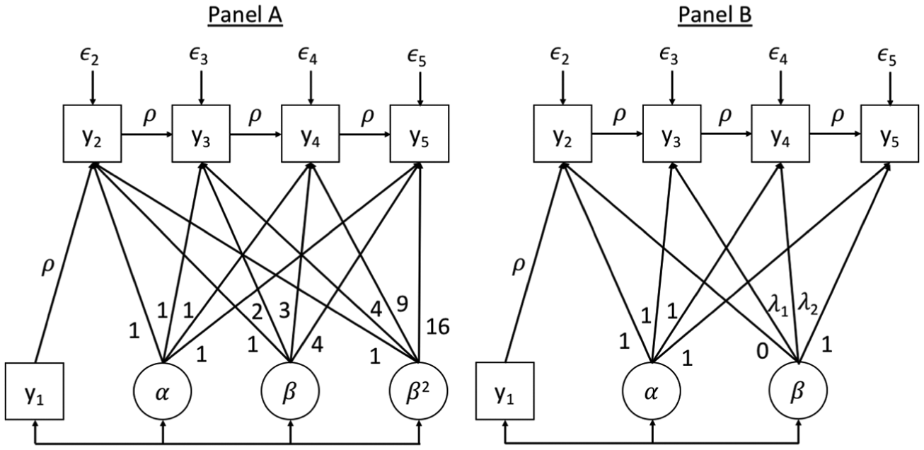
Unconditional univariate quadratic nonlinear autoregressive latent trajectory (NLALT) model with constrained autoregressive parameter (panel A) and unconditional univariate latent basis NLALT model with constrained autoregressive parameter (panel B) illustrated with five waves of data.

The latent basis (or freed loading) NLALT model has the same model equation and standard assumptions as the linear ALT model; the difference lies in the specification of the factor loadings for the random slope component, Λ_t. Rather than constraining the loadings to represent a linear trajectory, two loadings are fixed to 0 and 1, respectively, and the remaining loadings are freed to be estimated. Researchers are free to choose any two loadings to fix to 0 and 1, but in practice there are two common options. The first option is to set the first loading (note that this is for time point 2 when y_i₁ is treated as predetermined) to 0 and the second loading to 1 (Meredith and Tisak 1984, 1990). The second option is to set the first loading to 0 and the last loading to 1 (McArdle 1988). Either specification allows for flexible, nonlinear trajectories indexed by the change between the first and second loading or between the first and last loading, respectively.

For both the quadratic NLALT and the latent basis NLALT we adopt the specification developed by Bollen and Curran (2004) that treats the first wave, y_i₁, as predetermined. As noted above with the linear ALT model, it is possible to treat the first wave as endogenous, but this option is rarely used.

Following Bianconcini and Bollen (2018), it can be useful to rearrange the NLALT equations to appreciate their interpretation. One rearrangement of equation (2), for instance, is given by

y_{it} - α_{i} - Λ_{1 t} β_{i} - Λ_{2 t} β_{i}^{2} = ρ_{t, t - 1} y_{i, t - 1} + ϵ_{it} .

(3)

In this form we subtract the individual-specific trajectory components—the random intercept, random slope, and random quadratic slope—from y_it, and the remaining component is the autoregressive process. This form illustrates one interpretation that the prior value of y predicts what remains after accounting for the trajectory. Similarly, we can also rearrange equation (2) as

y_{it} - ρ_{t, t - 1} y_{i, t - 1} = α_{i} + Λ_{1 t} β_{i} + Λ_{2 t} β_{i}^{2} + ϵ_{it} .

(4)

In this form, we see that the model allows for a possible quadratic trajectory after accounting for an autoregressive process. These equations highlight that the key to interpreting NLALT models lies in recognizing that the individual-specific trajectory component is net of the autoregressive component (and vice versa). Which particular interpretation to emphasize depends on the substantive context and hypotheses concerning the presence of both types of longitudinal processes.

As with the linear ALT model, it is possible to include time-invariant predictors of the latent trajectory components of the model and the predetermined first wave.² The conditional univariate quadratic NLALT model adds the following equations to equation (2):

y_{i 1} = ν + π_{y 1}^{’} z_{i} + ϵ_{i y_{1}}

(5)

α_{i} = μ_{α} + π_{α}^{’} z_{i} + ζ_{i α}

(6)

β_{i} = μ_{β} + π_{β}^{’} z_{i} + ζ_{i β}

(7)

β_{i}^{2} = μ_{β^{2}} + π_{β^{2}}^{’} z_{i} + ζ_{i β^{2}},

(8)

where z_i is a vector of time-invariant predictors and the four vectors of pi parameters (i.e., $π_{y 1}, π_{α}, π_{β}, {π_{β}}^{2}$ ) capture the associations between the time-invariant covariates and each component of the latent trajectory and the predetermined first wave. In particular, the regression coefficients capture shifts in the conditional means of the latent trajectory components of the model and a shift in the conditional mean of the predetermined wave. The conditional univariate latent basis NLALT model adds equations (5), (6), and (7) to equation (1).

3.1. Model Identification

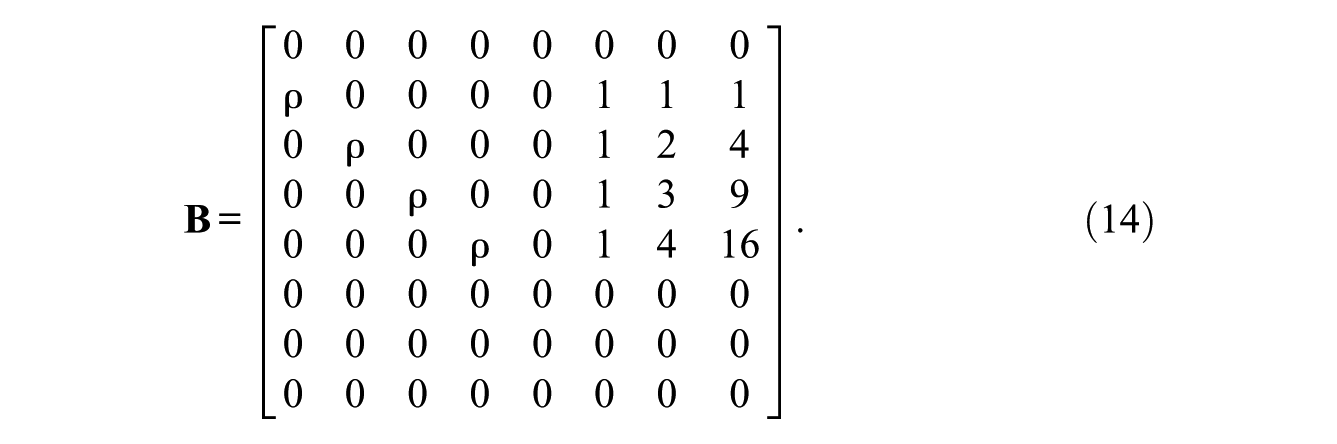
Bollen and Curran (2004) provide general matrix equations and implied moment matrices for ALT models that we use to establish the global identification—whether or not it is possible to find a unique set of parameter estimates—of the NLALT models. The general equations for ALT models are given by

η_{i} = μ + B η_{i} + ζ_{i}

(9)

o_{i} = P η_{i} .

(10)

In these expressions η_i is a vector that includes the repeated measures and the random trajectory components, µ is a vector of means or intercepts, B is a coefficient matrix that captures the effects of η_i on each other, and ζ_i is a vector of error terms for the variables in η_i. The second equation functions to select the observed variables (o_i) from the latent variables in η_i using a selection matrix P. These equations can be used to find the implied moment matrices for ALT models; see Bollen and Curran (2004) for derivations:

μ (θ) = P (I - B)^{- 1} μ

(11)

\sum (θ) = P (I - B)^{- 1} \sum_{ζ ζ} (I - B)^{- 1 ’} P ’,

(12)

where I is an identity matrix and θ is a vector of model parameters.³

We establish global model identification for an unconditional univariate quadratic NLALT and for an unconditional univariate latent basis NLALT with the autoregressive parameter constrained to be equal across all waves and with the first wave treated as predetermined. These represent baseline parameterizations of the two forms of NLALT models.

3.1.1. Quadratic NLALT Model

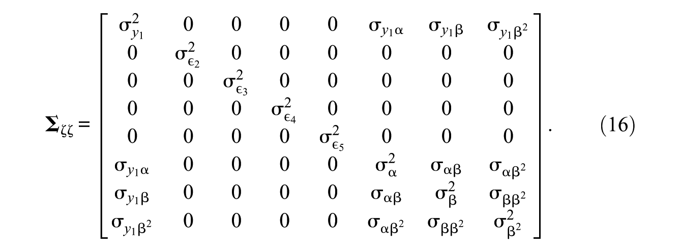
The parameters for the unconditional univariate quadratic NLALT model include the means, variances, and covariances among the three components of the latent trajectories ( $μ_{α}, μ_{β}, μ_{β^{2}}, σ_{α}^{2}, σ_{β}^{2}, σ_{β^{2}}^{2}, σ_{α β}, σ_{α β^{2}}, σ_{β β^{2}}$ ), the mean and variance for the predetermined wave ( $μ_{y_{1}}, σ_{y_{1}}^{2}$ ), the covariances between the predetermined wave and the components of the latent trajectories ( $σ_{y_{1} α}, σ_{y_{1} β}, σ_{y_{1} β^{2}}$ ), the autoregressive parameter constrained to be equal across waves (ρ), and T− 1 error variances for the endogenous repeated measures ( $σ_{ϵ_{2}}^{2}, \dots σ_{ϵ_{T}}^{2}$ ). This gives us 15 + (T− 1) parameters to estimate. Based on the t-rule, we need a minimum of five waves of data to potentially identify the quadratic NLALT model (Bollen 1989).

We rely on algebraic methods to solve for all of the model parameters using the implied moment matrices in equations (11) and (12) to establish the global identification status of the the unconditional univariate quadratic NLALT model with the autoregressive parameter constrained to be equal across all waves, with the first wave treated as predetermined, and with five waves of data. The matrices in equations (11) and (12) are specified as follows. P and B are given by

P = [\begin{matrix} 1 & 0 & 0 & 0 & 0 & 0 & 0 & 0 \\ 0 & 1 & 0 & 0 & 0 & 0 & 0 & 0 \\ 0 & 0 & 1 & 0 & 0 & 0 & 0 & 0 \\ 0 & 0 & 0 & 1 & 0 & 0 & 0 & 0 \\ 0 & 0 & 0 & 0 & 1 & 0 & 0 & 0 \end{matrix}]

(13)

and

B = [\begin{matrix} 0 & 0 & 0 & 0 & 0 & 0 & 0 & 0 \\ ρ & 0 & 0 & 0 & 0 & 1 & 1 & 1 \\ 0 & ρ & 0 & 0 & 0 & 1 & 2 & 4 \\ 0 & 0 & ρ & 0 & 0 & 1 & 3 & 9 \\ 0 & 0 & 0 & ρ & 0 & 1 & 4 & 16 \\ 0 & 0 & 0 & 0 & 0 & 0 & 0 & 0 \\ 0 & 0 & 0 & 0 & 0 & 0 & 0 & 0 \\ 0 & 0 & 0 & 0 & 0 & 0 & 0 & 0 \end{matrix}] .

(14)

µ and Σ_ζζ are given by

μ = [\begin{matrix} μ_{y_{1}} \\ 0 \\ 0 \\ 0 \\ 0 \\ μ_{α} \\ μ_{β} \\ μ_{β^{2}} \end{matrix}]

(15)

and

\sum_{ζ ζ} = [\begin{matrix} σ_{y_{1}}^{2} & 0 & 0 & 0 & 0 & σ_{y_{1} α} & σ_{y_{1} β} & σ_{y_{1} β^{2}} \\ 0 & σ_{ϵ_{2}}^{2} & 0 & 0 & 0 & 0 & 0 & 0 \\ 0 & 0 & σ_{ϵ_{3}}^{2} & 0 & 0 & 0 & 0 & 0 \\ 0 & 0 & 0 & σ_{ϵ_{4}}^{2} & 0 & 0 & 0 & 0 \\ 0 & 0 & 0 & 0 & σ_{ϵ_{5}}^{2} & 0 & 0 & 0 \\ σ_{y_{1} α} & 0 & 0 & 0 & 0 & σ_{α}^{2} & σ_{α β} & σ_{α β^{2}} \\ σ_{y_{1} β} & 0 & 0 & 0 & 0 & σ_{α β} & σ_{β}^{2} & σ_{β β^{2}} \\ σ_{y_{1} β^{2}} & 0 & 0 & 0 & 0 & σ_{α β^{2}} & σ_{β β^{2}} & σ_{β^{2}}^{2} \end{matrix}] .

(16)

Substituting these into equations (11) and (12) generates a 5 × 1 vector of equations for the implied mean vector and a 5 × 5 matrix of equations for the implied covariance matrix that relate all of the model parameters to the means and covariances of the five observed repeated measures. The system of equations is difficult to solve by hand; thus we used Maple to ensure that a unique solution exists for each parameter (Bollen and Bauldry 2010; MapleSoft 2017). For those interested, a Maple worksheet is maintained at https://github.com/sbauldry/nlalt that includes a set of algebraic solutions for all model parameters.

This demonstrates that the unconditional univariate quadratic NLALT model with the autoregressive parameter constrained to be equal across all waves and with the first wave treated as predetermined is globally identified with five or more waves of data.⁴ Additional waves of data may allow the autoregressive parameter to vary across waves or other alterations to the baseline specification of the quadratic NLALT model. In practice, we suggest following the identification rules we give in this paper followed by the usual local identification check that determines whether the information matrix is singular (Rothenberg 1971). This latter empirical check on local identification is available in nearly all structural equation modeling (SEM) software. If uncertainty about identification remains, the computer algebra approach to establishing model identification that we used here and that is described in Bollen and Bauldry (2010) is another option.

3.1.2. Latent Basis NLALT Model

The parameters for the unconditional univariate latent basis NLALT model include the means, variances, and covariances among the two components of the latent trajectories ( $μ_{α}, μ_{β}, σ_{α}^{2}, σ_{β}^{2}, σ_{α β}$ ), the mean and variance for the predetermined wave ( $μ_{y_{1}}, σ_{y_{1}}^{2}$ ), the covariances between the predetermined wave and the components of the latent trajectories ( $σ_{y_{1} α}, σ_{y_{1} β}$ ), the autoregressive parameter constrained to be equal across waves (ρ), T− 3 factor loadings that depend on which waves are constrained to 0 and 1, and T– 1 error variances for the endogenous repeated measures ( $σ_{ϵ_{2}}^{2}, \dots σ_{ϵ_{T}}^{2}$ ). This gives us 10 + (T− 3) + (T− 1) parameters to estimate. Based on the t-rule, we need a minimum of four waves of data to potentially identify the latent basis NLALT model.

The same procedure was used with the quadratic NLALT model to establish the global identification of the latent basis NLALT model. We obtained a set of solutions for all of the parameters with four waves of data (see https://github.com/sbauldry/nlalt for the specific solutions).⁵ With four waves of data, however, the latent basis NLALT model is exactly identified, and thus no degrees of freedom are available for testing the overall fit of the model.

3.2. Estimation and Testing

The NLALT is a longitudinal model that refers to the equations and assumptions that capture it. Practically speaking, the estimation and testing of this model is easiest to undertake in an SEM framework. The SEM framework is useful in that it permits the latent basis (or freed loading) model that cannot be currently fit with other longitudinal approaches (e.g., a multilevel or random-effects framework). In addition, the SEM approach provides a straightforward method for maximum likelihood estimation of the model along with nested comparisons of the fit of this model to a variety of competing longitudinal structures. Among these tests is a comparison of each longitudinal model to a saturated model, and this test is typically not available in a non-SEM framework. Furthermore, the SEM approach has fit indices that are helpful in supplementing the likelihood ratio comparisons of fit. A variety of SEM software packages are available, such as Mplus (Muthén and Muthén 2012), AMOS (Arbuckle 2006), and LISREL (Jöreskog and Sorbom 2005), and SEMs can also be fit in general statistical software, such as as the lavaan package of R (Rosseel 2012) and the SEM and GSEM commands in Stata (StataCorp 2017).

The full information maximum likelihood (FIML) fitting function is given by

F_{ML} = \ln | \sum (θ) | + tr [\sum^{- 1} (θ) S] - \ln | S | - p + (\bar{z} - μ (θ)) ’ \sum^{- 1} (θ) (\bar{z} - μ (θ)),

(17)

where θ is a vector of parameters, Σ(θ) and µ(θ) are the implied moment matrices, S and $\bar{z}$ are the sample covariance matrix and mean vector, respectively, and p is the number of observed variables. Although the FIML estimator is derived under the assumption of multivariate normality, corrections to the test statistics and standard errors are readily available under nonnormality (Bollen and Stine 1990, 1993; Browne 1984; Satorra 1990).

For overidentified models, researchers can rely on standard model fit statistics based on the assumption of multivariate normality and indices for structural equation models to assess the overall fit of the model with the data. Under the null hypothesis, H₀ : Σ = Σ(θ) and µ = µ(θ), where Σ and µ are the population covariance matrix and mean vector, and the test statistic T = (N – 1)F_ML has an asymptotic chi-square distribution with degrees of freedom equal to [p(p+ 1)/2 +p] –t, where t is the number of estimated parameters. If a researcher suspects excess kurtosis or has other reasons to relax the assumption of multivariate normality, then the bootstrap or Satorra-Bentler correction can be used to obtain a chi-square test statistic (Bollen and Stine 1993; Satorra 1990).

Other useful fit statistics include information theoretic indices, such as the Bayesian information criteria (BIC) (Raftery 1995; Schwarz 1978). Various baseline fit indices in which the chi-square of the hypothesized model is compared with that of a baseline model, such as the incremental fit index (Bollen 1989), the Tucker-Lewis index (TLI; Tucker and Lewis 1973), and the relative noncentrality index and the closely related comparative fit index (CFI; Bentler 1990), are provided in most SEM software. The root mean square error of approximation (RMSEA; Steiger and Lind 1980) is a “stand-alone” measure of model fit. In general, lower values of information theoretic indices, such as the BIC, indicate better fit, and values less than 0 of the BIC in the form provided by Raftery (1995) indicate a hypothesized model has a better fit with the data than the saturated model. For baseline fit indices, there are different rules of thumb, but in general, values closer to 1 indicate good fit with the data. Finally, for the RMSEA, values closer to 0, with 0.05 as a common threshold, indicate good fit with the data. As with any structural equation model, we recommend assessing model fit using an array of fit statistics as they each have different desirable and undesirable properties.

3.3. Model Comparisons

There are a number of potential model comparisons that researchers might be interested in testing. The linear ALT is a restricted version of the quadratic NLALT in which the mean, variance, and covariances involving the quadratic component of the latent trajectory are constrained to 0. Therefore, it is possible to use standard chi-square difference tests to compare the fit of the linear ALT and the quadratic NLALT. The standard quadratic growth curve model, however, is not a restricted form of the quadratic NLALT when the first wave is treated as predetermined. It is possible, though, to test a variant of the quadratic NLALT model in which the autoregressive parameter is constrained to be 0 across all waves. Although this is not identical to the quadratic growth curve model, if it fits the data as well as the quadratic NLALT model with autoregressive parameter(s), then researchers may wish to consider a standard quadratic growth curve model. Finally, a standard autoregressive model is a restricted version of the quadratic NLALT model with the means, variances, covariances, and factor loadings from the latent trajectory components constrained to 0.

Similar to the situation with the quadratic NLALT model, the linear ALT model is a restricted version of the latent basis (freed loading) NLALT model in which the freed factor loadings are constrained to follow a linear pattern as in the linear ALT model. The latent basis trajectory model, however, is not a restricted version of the latent basis NLALT model with a predetermined wave 1. Once again, however, it is possible to test a version of the latent basis NLALT model with the autoregressive parameter(s) constrained to 0. Finally, as with the quadratic NLALT model, a standard autoregressive model is a restricted version of the latent basis NLALT model with the trajectory components removed.

Beyond formal chi-square difference tests, it is possible to compare the fit across nonnested models that have the same sample and variables using the various fit indices and the BIC or AIC.

4. Simulation Study

This section presents the results of a simulation study designed to illustrate the potential bias that can arise from fitting some of the alternative models for longitudinal processes to data generated to have both an autoregressive process and nonlinear case-specific trajectories.

4.1. Simulation Design

We used Stata 15 (StataCorp 2017) to generate 500 data sets with 5,000 cases each based on the following data-generating model. The exogenous variables, the first wave of data (y₁), the latent intercept (α), the latent linear component (β), and the latent quadratic component (β²) were drawn from a multivariate normal distribution with a mean vector and covariance matrix

μ = [\begin{matrix} 0 \\ 0 \\ 1 \\ 2 \end{matrix}] \sum = [\begin{matrix} 0.1 & 0 & 0 & 0 \\ 0 & 1.5 & 0 & 0 \\ 0 & 0 & 0.3 & 0 \\ 0 & 0 & 0 & 0.1 \end{matrix}] .

(18)

The vector of means indicates a quadratic growth process that begins at 0. The variances of the growth parameters are based on our past experience with these models and in particular reflect the relatively small degrees of variance in the linear and quadratic components we often observe. We generated four additional waves of data with a fixed autoregressive parameter of 0.2 using

y_{2} = α + β + β^{2} + 0.2 y_{1} + ϵ_{2}

(19)

y_{3} = α + 2 β + 4 β^{2} + 0.2 y_{2} + ϵ_{3}

(20)

y_{4} = α + 3 β + 9 β^{2} + 0.2 y_{3} + ϵ_{4}

(21)

y_{5} = α + 4 β + 16 β^{2} + 0.2 y_{4} + ϵ_{5} .

(22)

The error terms were drawn from normal distributions with mean 0 and variances 0.15, 2, 3, and 4, respectively. The variance of y₁ and the error terms for y₂ through y₅ were chosen for numerical stability and to ensure R²s ranging from about .75 to .90 for the four endogenous waves, which, again, is similar to values we have observed in empirical work.

Following data generation, we fit four models to each of the 500 data sets in Mplus 7 (Muthén and Muthén 2012) and stored model fit statistics and parameter estimates for further analysis in Stata. The four models included (1) a correctly specified quadratic NLALT model, (2) a linear ALT model, (3) a (modified) quadratic latent curve model with the first wave treated as exogenous, and (4) a standard autoregressive model. All of the code for this simulation is maintained at a publicly available code repository (https://github.com/sbauldry/nlalt).

4.2. Simulation Results

Table 1 reports average model fit statistics across the 500 replications for each model. As expected, the chi-square test statistic for the quadratic NLALT model indicates good fit and corresponds with the theoretical proportion of 0.05 statistically significant tests across the 500 replications. The chi-square test statistic is statistically significant in all replications for all of the alternative models, though it is relatively low for the quadratic latent curve model. The BIC also provides a clear signal on average that the linear ALT and the standard autoregressive models do not have a good fit with the data. Once again, the BIC is relatively lower, though still positive and indicative of poor fit in general, for the quadratic latent curve model. In contrast to the other fit statistics, the CFI and TLI on average indicate reasonable fit for all of the models. The RMSEA is high for the linear ALT and the standard autoregressive but falls below the conventional 0.05 cutoff for the quadratic latent curve model. Overall, with this particular data-generating model, we could easily imagine choosing the quadratic latent curve as having a sufficiently good fit with the data and even potentially the linear ALT or the standard autoregressive model if we had not considered an NLALT model or did not pay much attention to the chi-square test or the BIC.

Table 1.

Mean of Model Fit Statistics for Simulation Models

Model	χ²	Pr Sig	BIC	CFI	TLI	RMSEA
Quadratic NLALT	6.98	.05	−52.64	1.00	1.00	.003
Linear ALT	512.00	1.00	435.35	.97	.97	.11
Quadratic latent curve	87.96	1.00	19.83	1.00	.99	.04
Autoregressive	647.68	1.00	571.03	.96	.96	.12

Note: Pr Sig indicates the proportion of 500 replications in which the chi-square test statistic was statistically significant at the .05 level. For a small proportion, .018, of the quadratic latent curve models, Mplus issued a warning for the presence of a nonpositive definite covariance matrix for the latent variables. ALT = autoregressive latent trajectory; BIC = Bayesian information criterion; CFI = comparative fit index; NLALT = nonlinear autoregressive latent trajectory; RMSEA = root mean square error of approximation; TLI = Tucker-Lewis index.

Figure 2 reports the averages (and ±2 standard deviations) for selected parameter estimates related to the growth processes that are present in each of the four different models. Panels (a) through (d) report the average estimates for the autoregressive parameter and the means of the latent intercept, linear term, and quadratic term across the appropriate models. In panel (a), we see that the quadratic NLALT recovers the data-generating parameter of 0.2, but both the linear ALT and the standard autoregressive models substantially overestimate the parameter with estimates ranging between 1 and 1.3. An estimate of an autoregressive parameter that is greater than 1 implies an unstable autoregressive process and may be a sign of model misspecification, such as failing to include an individual-specific trajectory component of the growth process.

Figure 2.

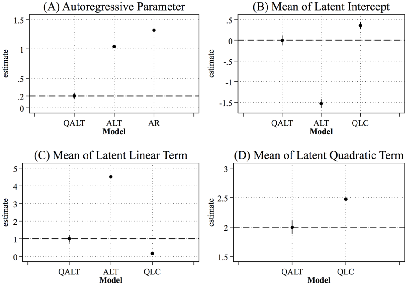
Selected parameter estimates from simulation study.

In panels (b) and (c), we see that the linear ALT model substantially underestimates the mean of the latent intercept and overestimates the mean of the latent linear term. Taken in combination with the overestimation of the autoregressive parameter, it is clear that the linear ALT model does a poor job of recovering several of the key parameters from the data-generating model. Similarly, in panels (b), (c), and (d), we see that the quadratic latent curve model overestimates the mean of the latent intercept and the mean of the latent quadratic term while underestimating the mean of the linear term. The bias in the parameter estimates is noticeably lower for the quadratic latent curve model compared with the linear ALT model, which is consistent with the better fit statistics observed for the quadratic latent curve model. Nonetheless, the differences in the average estimates of the quadratic latent curve model from the data-generating model lead to visibly different predicted average trajectories of growth.

4.3. Simulation Discussion

The aim of this simulation study is to demonstrate the potential bias that can arise in the parameters related to the trajectory component of various alternative longitudinal models if fit to data that come from a process involving both an autoregressive component and a nonlinear case-specific trajectory component. It is apparent in this case that a failure to account for either an autoregressive process or a nonlinear individual-specific growth process results in substantially biased estimates of the growth parameters in the model as they compensate for the growth parameters that have been left out. Furthermore, in this case, the evidence for model misspecification is not particularly strong for the quadratic latent curve model.

The aim of this simulation study, however, is not to suggest that bias in parameter estimates will always manifest in these particular patterns or be as significant. It is possible that a misspecified trajectory model that either misses an autoregressive process that is present in the data or a nonlinear growth process that is present in the data could provide substantively adequate fit for analytical purposes. In addition, we have examined only a single data-generating model to illustrate potential bias. Future studies could extend the simulation to consider a range of data-generating models with the goal of identifying boundaries of parameter values that lead to more bias or to less.

5. Empirical Example

This section illustrates the utility of the quadratic and latent basis NLALT models with an empirical example modeling trajectories of growth in weight in two-month intervals from birth to two years old. Trajectories of weight may involve both individual-specific growth processes and autoregressive processes. External shocks to weight from, for instance, an acute illness may have a short-term impact on trajectories of weight that fits with an autoregressive process. In addition, different infants follow different trajectories of weight for a host of genetic, biological, and environmental reasons that can be modeled as individual-specific growth processes. Furthermore, growth in weight is known to follow a nonlinear trajectory among infants (WHO Multicentre Growth Reference Study Group 2006). Characteristics of mothers, such as age and smoking status, are also known to be a factor in birth weight as well as trajectories of growth (Aldous and Edmonson 1993; Conter et al. 1995). Modeling trajectories of weight thus represents a good candidate for NLALT models.

The data for the empirical example come from the Cebu Longitudinal Health and Nutrition Survey (CLHNS), which followed a cohort of children born in Cebu, Philippines, in the 1980s (Adair et al. 2011). The CLHNS began with a baseline survey in 1983 and 1984 of 3,327 expectant mothers in 33 randomly selected communities in the Cebu metropolitan area. Anthropomorphic measures of the children were collected every two months for the first two years following birth, for a total of 13 waves of data. Our analysis focuses first on developing models for weight trajectories for girls and then on introducing covariates predicting the parameters of the model for weight trajectories.

At birth there are data on the birth weights of 1,434 females. By wave 12, 278 females have been lost to attrition (19 percent). We use a FIML estimator that allows us to maintain all of the cases under the assumption that the data are missing at random (Arbuckle 1996). Although we have strong substantive reasons to expect nonlinear weight trajectories, it is still important to check this in the data. Figure 3 illustrates the trajectory of average weights across waves (thick black line) and individual trajectories for 50 randomly selected cases among those with data for all waves (thin gray lines). As expected, the figure indicates weight trajectories are nonlinear, with an early period characterized by relatively fast weight gain and then a later period beginning around age six months with a slower rate of gain. In addition, there appears to be a reasonable amount of variation around the average trajectory, and variation increases over time.

Figure 3.

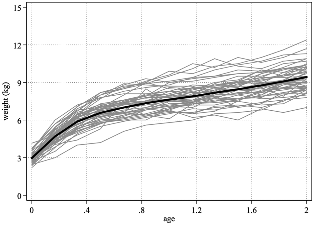
Trajectories of weight from birth to age 2 among females in the Cebu Longitudinal Health and Nutrition Survey.

5.1. Unconditional Model Specification

The initial analysis considers six models of weight trajectories: (1) a (modified) quadratic latent curve model, (2) a (modified) latent basis model, (3) a standard autoregressive model, (4) a linear ALT model, (5) a quadratic NLALT model, and (6) a latent basis NLALT model. Although the waves of data collection occurred at regular intervals, the weights of individuals were measured in a range of days around these regular intervals. For instance, at the second wave, which occurred roughly four months after birth, individuals were weighed anywhere from three days prior to the four-month mark to eight days following the four-month mark. Because these differences are meaningful in terms of capturing weight trajectories in this age range, we augment all of the growth models with an additional term, labeled Δage, that captures the difference in days between the set point for the wave and the actual age at which individuals were weighed.

For this analysis, the quadratic NLALT model is specified as

{weight}_{it} = α_{i} + Λ_{1 t} β_{i} + Λ_{2 t} β_{i}^{2} + ρ_{t, t - 1} {weight}_{i, t - 1} + γ_{t} (Δ age)_{it} + ϵ_{it},

(23)

for t = 1, . . . , 12 with t = 0 (i.e., birth) treated as predetermined. We constrain the autoregressive parameters for the 12 waves to be equal due to the fixed time period between each wave (two months). We set the factor loadings for the linear slope parameter to be fractions of a year that correspond to the ages at which the waves occurred,

Λ_{1 t} = [2 / 12, 4 / 12, . . ., 24 / 12],

(24)

and square each element of Λ_1t to obtain Λ_2t.

We specify a quadratic latent growth curve model by starting with equation (23) and fixing the autoregressive parameters, ρ_t,t−1, to be 0 for all waves. This is a modified version of the standard quadratic latent growth curve model that treats the first wave (birth weight) as predetermined and thus maintains the nested structure (i.e., the quadratic latent growth curve model is a restricted version of the quadratic NLALT model) allowing for a chi-square difference test. We specify a standard autoregressive model by constraining the means, variances, covariances, and factor loadings from the latent trajectory components to 0. Finally, we specify the linear ALT model by setting Λ_2t = 0, setting the mean and variance of β_i² to 0, and setting all covariances between β_i² and other exogenous variables (α_i, β_i, weight_i₀, Δage_it) to 0.

For this analysis, the latent basis NLALT model is specified as

{weight}_{it} = α_{i} + Λ_{1 t} β_{i} + ρ_{t, t - 1} {weight}_{i, t - 1} + γ_{t} (Δ age)_{it} + ϵ_{it} .

(25)

As with the quadratic NLALT, we constrain the autoregressive parameters for the 12 waves to be equal due to the fixed time period between each wave (two months). We set the first and last factor loadings for the slope parameter to be 0 and 1, respectively, and allow the other loadings to be estimated,

Λ_{1 t} = [0, Λ_{2}, . . ., Λ_{11}, 1] .

(26)

We specify a latent basis model by starting with equation (25) and fixing the autoregressive parameters, ρ_t,t−1, to be 0 for all waves. As with the quadratic latent growth curve model, this is a modified version of the standard latent basis model that treats the first wave (birth weight) as predetermined and thus maintains the nested structure allowing for a chi-square difference test.

5.2. Conditional Model Specification

In addition to modeling trajectories, social scientists are often interested in analyzing covariates that may be associated with trajectories (either as predictors of trajectories or as outcomes of trajectories). To illustrate one of these possibilities, we extend our analysis of weight trajectories to include mother’s age and smoking status. The model starts with the best model for weight trajectories and includes the two covariates predicting the trajectory components.

As will be shown, the quadratic NLALT model provides the best-fitting model for weight trajectories. We extend this model to include covariates predicting the weight trajectory components

{weight}_{it} = α_{i} + Λ_{1 t} β_{i} + Λ_{2 t} β_{i}^{2} + ρ_{t, t - 1} {weight}_{i, t - 1} + γ_{t} (Δ age)_{it} + ϵ_{it}

(27)

{weight}_{i 0} = π_{00} + π_{01} youn g_{i} + π_{02} ol d_{i} + π_{03} smok e_{i} + ζ_{0 i}

(28)

α_{i} = π_{10} + π_{11} youn g_{i} + π_{12} ol d_{i} + π_{13} smok e_{i} + ζ_{α i}

(29)

β_{i} = π_{20} + π_{21} youn g_{i} + π_{22} ol d_{i} + π_{23} smok e_{i} + ζ_{β i}

(30)

β_{i}^{2} = π_{30} + π_{31} youn g_{i} + π_{32} ol d_{i} + π_{33} smok e_{i} + ζ_{β^{2} i},

(31)

where young_i and old_i are respective indicators for mothers who were younger than 20 or older than 35 when they gave birth to the child in the study (the referent is mothers between 20 and 35), and smoke_i is an indicator for mothers who smoked during pregnancy. The model specifies birth weight, the latent intercept, the latent linear component of the slope, and the latent quadratic component of the slope as predicted by the three indicators capturing characteristics of the mothers thought to influence birth weight and trajectories of weight. In addition, the disturbances for each of the growth components, $ζ_{0 i}, ζ_{α i}, ζ_{β i}, ζ_{β^{2} i}$ , are allowed to be correlated. The latent basis NLALT model can be extended in a similar fashion to include predictors of the growth components.

The CLHNS data for this example were prepared for analysis using Stata 15 (StataCorp 2017), and the various trajectory models were fit using Mplus 7 (Muthén and Muthén 2012). Information about obtaining the CLHNS data can be found at http://www.cpc.unc.edu/projects/cebu. The online appendix includes Mplus code for the NLALT models. All of the remaining code used in this analysis is maintained at a publicly available repository (https://github.com/sbauldry/nlalt).

5.3. Results

Table 2 reports model fit statistics for the six different unconditional trajectory models. We see that the modified quadratic latent growth curve model and the modified latent basis model show poor fit across all of the model fit statistics. The chi-square test statistics are large and statistically significant, the BICs are positive (which indicates the saturated model is preferred over the hypothesized model), the CFI and TLI are below 0.9, and the RMSEA is above 0.1. The fit statistics for these two models all point to problems with model specification.

Table 2.

Model Fit Statistics for Different Models for Weight Trajectories

Model	χ²	df	p	BIC	CFI	TLI	RMSEA
Quadratic latent curve	5730.23	174	.000	4465.56	.80	.74	.15
Latent basis	4105.40	181	.000	2789.85	.86	.83	.12
Autoregressive	848.73	209	.000	−670.33	.98	.98	.05
Linear ALT	815.38	190	.000	−565.58	.98	.97	.05
Quadratic NLALT (a)	378.15	173	.000	−879.25	.99	.99	.03
Latent basis NLALT (a)	508.95	180	.000	−799.33	.99	.99	.04
Quadratic NLALT (b)	379.59	174	.000	−885.08	.99	.99	.03
Latent basis NLALT (b)	560.95	195	.000	−856.35	.99	.99	.04

Note: The quadratic latent curve and latent basis models are modified versions of the standard models that treat the first wave (birth) as predetermined. The quadratic and latent basis NLALT models with the (a) labels refer to the standard specification outlined in the text. The quadratic and latent basis NLALT models with the (b) labels refer to the alternative specifications that address the negative variance estimates or estimates of correlations greater than one as discussed in the text. ALT = autoregressive latent trajectory; BIC = Bayesian information criterion; CFI = comparative fit index; NLALT = nonlinear autoregressive latent trajectory; RMSEA = root mean square error of approximation; TLI = Tucker-Lewis index.

The fit statistics for the autoregressive and the linear ALT model appear more reasonable. Although the chi-square test statistics are significant, the BICs are negative, the CFIs and TLIs are both around 0.98, and the RMSEAs are 0.05. An analyst might well conclude that either the autoregressive model or the linear ALT model fit the data sufficiently to proceed; however, both types of NLALT models provide an even better fit with the data. For both the quadratic and the latent basis NLALT models—labeled (a) in Table 2—the chi-square test statistics are significant, but the BICs are negative, the CFIs and TLIs are around 0.99, and the RMSEAs are below 0.05.

An inspection of the parameter estimates for both NLALT models, however, reveals issues that bear further investigation. In particular, in the quadratic NLALT model, the correlation between the latent linear slope variable and the quadratic slope variable is estimated to be −1.003. In the latent basis NLALT model, the variance for the latent slope variable is estimated to be −0.002. These estimates result in nonpositive definite covariance matrices for the latent variables, which is indicated in a warning issued by Mplus.

Such inadmissible estimates for variances or correlations are not that uncommon with structural equation models and may arise due to a variety of issues, including outliers or influential cases, sampling fluctuations, or structural misspecifications (Kolenikov and Bollen 2012). We first examined diagnostics for outliers (Mahalanobis distances) and influential cases (Cook’s D and an influence measure based on the log likelihood) and determined that these were unlikely to be the source of the inadmissible estimates. We then calculated a test statistic for whether the estimates differed significantly from admissible values (i.e., a correlation of −1.0 and a variance of 0) using standard errors based on the empirical sandwich estimator as recommended by Kolenikov and Bollen (2012) for sample sizes greater than 1,000. Because the inadmissible estimates for both models were not significantly different from admissible values, we concluded that the inadmissible estimates likely reflect sampling variation rather than structural misspecification.

One approach to addressing inadmissible estimates that are not significantly different from admissible values is to constrain the model parameters to slightly different values than the inadmissible estimates. For the quadratic NLALT model, we constrained the association between the latent linear slope and latent quadratic slope to be −0.06 (slightly larger than the original estimate of −0.04), which results in an admissible correlation between the two latent variables of −0.98 (slightly lower than −1.003). For the latent basis NLALT model, the estimated variance for the latent slope component of the trajectory is close to 0, so we constrain it to be 0 and constrain the covariances with the latent slope to also be 0. These minor model respecifications result in models with admissible parameter estimates (i.e., no negative variances or correlations less than −1) and fit statistics that continue to show good fit despite the inclusion of these additional constraints (see the models labeled [b] in Table 2).

Based on the model fit statistics reported in Table 2, particularly the BIC that can be compared across nonnested models,⁶ the quadratic NLALT and the latent basis NLALT dominate the other four model specifications. We can also conduct chi-square difference tests for the nested models (see Table 3). In this case, we begin with the respecified NLALT models described above and impose appropriate constraints to ensure that latent growth curve models, autoregressive model, or linear ALT model, respectively, are properly nested in the NLALT models. The chi-square difference tests corroborate the BICs and other model fit statistics in showing that the respecified quadratic NLALT and the respecified latent basis NLALT both have better fits with the data than any of the alternative growth models.

Table 3.

Chi-square Difference Tests for Nested Models for Weight Trajectories

Model	Δχ²	Δdf	p	ΔBIC
Quadratic latent curve vs. quadratic NLALT (b)	6032.52	1	.000	6016.25
Autoregressive vs. quadratic NLALT (b)	469.14	35	.000	214.75
Linear ALT vs. quadratic NLALT (b)	453.79	16	.000	319.50
Latent basis vs. latent basis NLALT (b)	8637.20	1	.000	8629.93
Autoregressive vs. latent basis NLALT (b)	287.78	14	.000	186.02
Linear ALT vs. latent basis NLALT (b)	947.16	10	.000	874.47

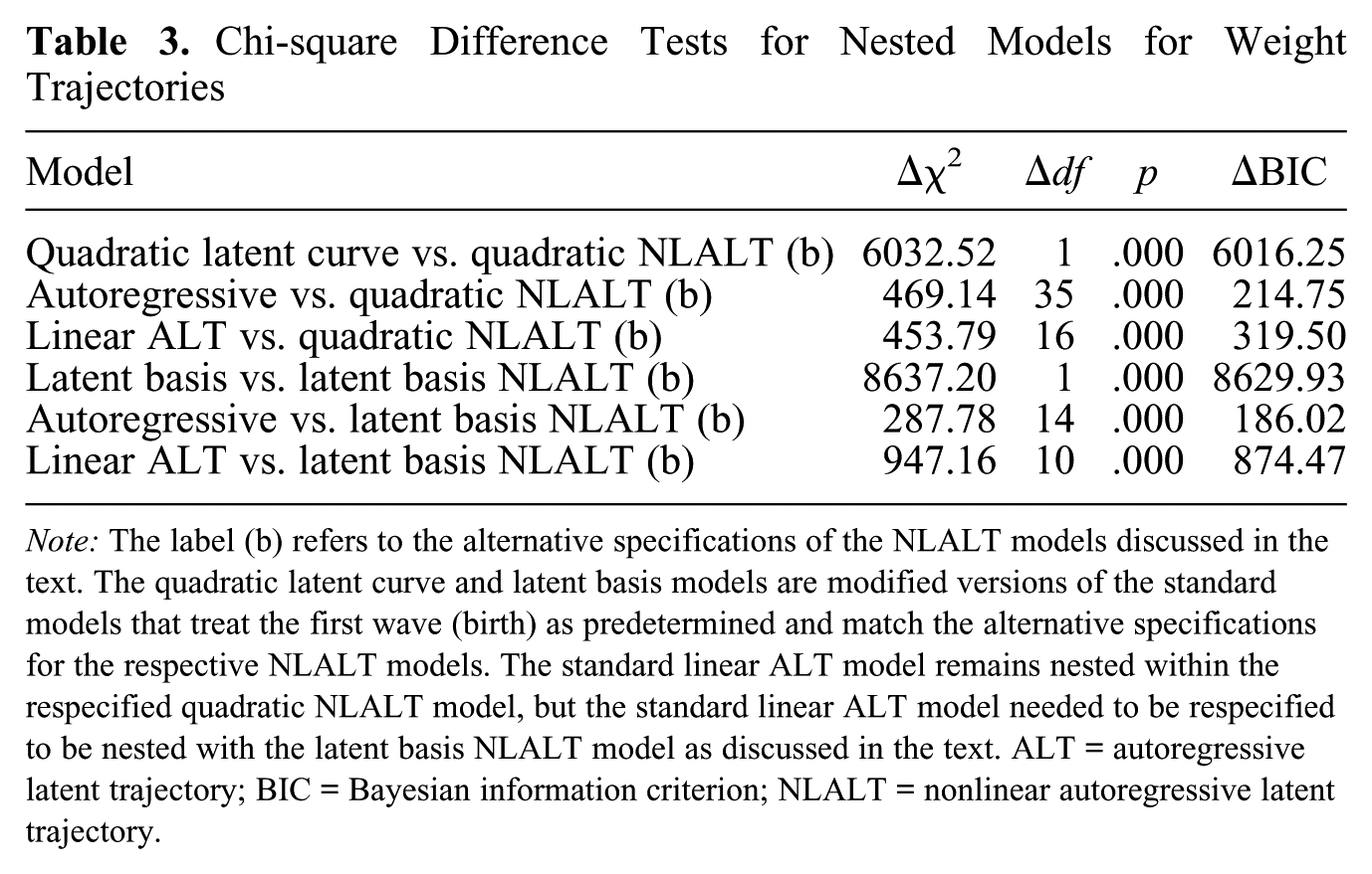
Note: The label (b) refers to the alternative specifications of the NLALT models discussed in the text. The quadratic latent curve and latent basis models are modified versions of the standard models that treat the first wave (birth) as predetermined and match the alternative specifications for the respective NLALT models. The standard linear ALT model remains nested within the respecified quadratic NLALT model, but the standard linear ALT model needed to be respecified to be nested with the latent basis NLALT model as discussed in the text. ALT = autoregressive latent trajectory; BIC = Bayesian information criterion; NLALT = nonlinear autoregressive latent trajectory.

Given that the respecified quadratic NLALT model has the best overall model fit statistics, we proceed with that model. Table 4 reports selected parameter estimates for the quadratic NLALT model (labeled QALT) and, as a point of comparison, estimates from the linear ALT model, the quadratic latent curve model, and the autoregressive model. Beginning with the parameter estimates for the growth components of the model, we see that the latent variables governing the individual-specific trajectories of weight have statistically significant means and variances, with the exception of the mean for the latent linear component of the trajectory. It is worth noting, however, that the quadratic latent variable has an estimate for the variance that is quite close to 0 (Var[β²] = 0.018). In some cases, it may be useful to fix this value to 0 (and the corresponding covariances with other variables to 0 as well) in order to improve the numerical stability of the model. We find that the autoregressive parameter is less than 1 (ρ = 0.619) and statistically significant as well. Finally, we note that the residual variances of the measures of weight across waves are all statistically significant (not reported), which indicates that age-specific error remains in the measures, though the R²s for these measures are generally quite high. The R²s range around 0.8 to 0.9, with the exception of 0.65 for the first wave.

Table 4.

Parameter Estimates for the Trajectory and Autoregressive Components of the Quadratic NLALT Model

Parameter	QALT	ALT	QLC	AR
µ_BW	2.961 (.011)	2.961 (.011)	2.961 (.011)	2.961 (.011)
Var(BW)	.187 (.007)	.187 (.007)	.187 (.007)	.187 (.007)
µ_α	2.878 (.026)	3.028 (.023)	4.910 (.027)	—
Var(α)	.136 (.009)	.158 (.008)	.609 (.030)	—
µ_β	−.080 (.057)	.751 (.015)	3.211 (.052)	—
Var(β)	.204 (.006)	.051 (.003)	2.043 (.109)	—
$μ_{β^{2}}$	.272 (.017)	—	−.526 (.021)	—
Var(β²)	.018 (.001)	—	.288 (.017)	—
ρ	.619 (.008)	.528 (.005)	—	.973 (.003)

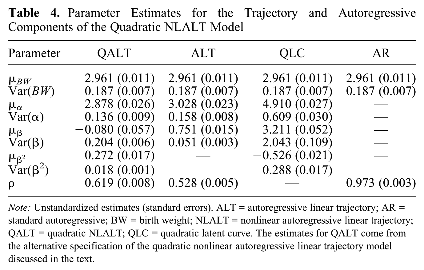
Note: Unstandardized estimates (standard errors). ALT = autoregressive linear trajectory; AR = standard autoregressive; BW = birth weight; NLALT = nonlinear autoregressive linear trajectory; QALT = quadratic NLALT; QLC = quadratic latent curve. The estimates for QALT come from the alternative specification of the quadratic nonlinear autoregressive linear trajectory model discussed in the text.

In terms of substantive interpretations, the estimate for the autoregressive parameter is relatively large. A 1.0 kg increase in weight in a given period is associated with a 0.6 kg increase in weight in the following 2 months net of the infant-specific trajectory of weight and holding the other covariates constant. The estimates for the components of the infant specific trajectories, µ_α = 2.878, µ_β = −0.080, and $μ_{β^{2}} = 0.272$ , indicate an accelerating rate of growth net of the autoregressive process and holding the other covariates constant. It is worth noting that these parameter estimates for the individual-specific quadratic trajectory at first glance might appear surprising as they imply a convex function as opposed to the slightly concave function evident in Figure 3. This underscores the importance of keeping in mind that these parameter estimates represent individual-specific trajectories net of an autoregressive process as discussed with equation (4) above. To see the average weight trajectory implied by the combination of the individual-specific growth component and the autoregressive process, we can plot the predicted average values of weight at each time point based on the full model and compare the trajectory with that observed in the data for a random subset of cases (see Figure 4). We see that the quadratic NLALT model appears to do an excellent job of capturing the average trajectory of weight among the infants.

Figure 4.

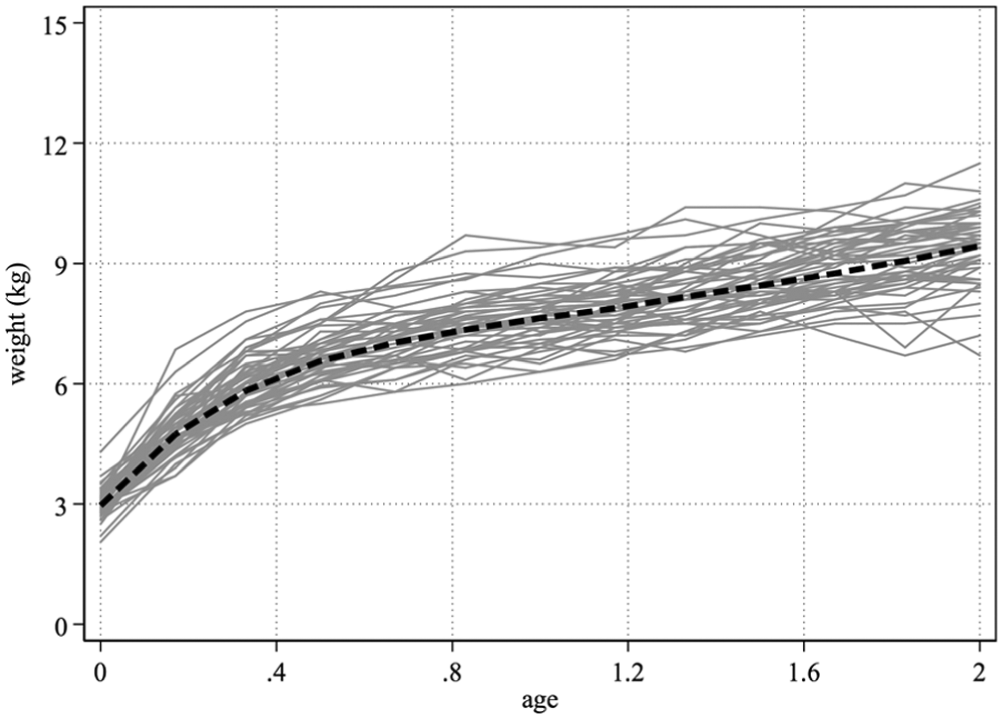
Predicted average weight trajectory from birth to age 2.

Turning to the alternative models, we see that, as expected, the estimates for the mean and variance of birth weight are the same across all models. The estimates for the remaining growth parameters, however, differ quite substantially across the alternative models. With the linear ALT model, we see a slightly higher estimate of the mean of the latent intercept and a slightly lower estimate of the autoregressive parameter with standard errors of roughly the same magnitude as the estimates from the quadratic NLALT model. There is a more substantial difference, however, in the mean of the latent linear component, which is positive as compared with a negative estimate in the quadratic NLALT. With the quadratic latent curve model, the absence of the autoregressive parameter leads to substantially different estimates for the means of the latent intercept, latent linear component, and latent quadratic component as compared with the estimates from the quadratic NLALT model. Finally, with the autoregressive model, the estimate for ρ is about 60 percent greater than the estimate for ρ from the quadratic NLALT model. In all cases, the combination of parameter estimates for the growth trajectories leads to different trajectories of weight across the four models and underscores the utility of the quadratic NLALT model in this analysis.

We continue with the respecified quadratic NLALT model and include the two mother’s characteristics—mother’s age and smoking status—as predictors of the birth weight (the predetermined first wave) and the latent trajectory components (the latent intercept, linear slope, and quadratic slope). Table 5 reports these parameter estimates. We see that both being under the age of 20 and smoking are associated with lower birth weights. We do not find any additional significant associations with the latent intercept (i.e., the time-invariant component of the individual-specific trajectories). We do, however, observe a significant negative association between smoking and the latent linear component of the trajectory and a significant positive association with the latent quadratic component of the trajectory. Keeping in mind that these represent associations net of the autoregressive component of the process, we can get a sense of the association of smoking with the individual-specific trajectory component of weight by examining the quadratic curve implied by the estimates across the range of ages. In this case, we find that smoking is associated with a negative influence on the growth trajectory net of the autoregressive process through age 2 (the last time point) as −0.187*2 + 0.063*2² = −0.122, though the negative influence on the rate of growth associated with mother’s smoking becomes less pronounced over time. The R²s for each of the growth components, however, indicate that these characteristics of the mothers do not explain much of the variance in each of the components.

Table 5.

Parameter Estimates for the Predictors of the Trajectory Components of the Quadratic NLALT Model

Variable	µ_BW	µ_α	µ_β	$μ_{β^{2}}$
Mother’s age < 20	−.153 (.033)	−.011 (.040)	−.087 (.069)	.028 (.029)
Mother’s age > 35	.018 (.040)	−.059 (.049)	−.002 (.083)	.011 (.034)
Mother smoked	−.086 (.033)	−.046 (.040)	−.187 (.069)	.063 (.028)
R ²	.019	.005	.024	.030

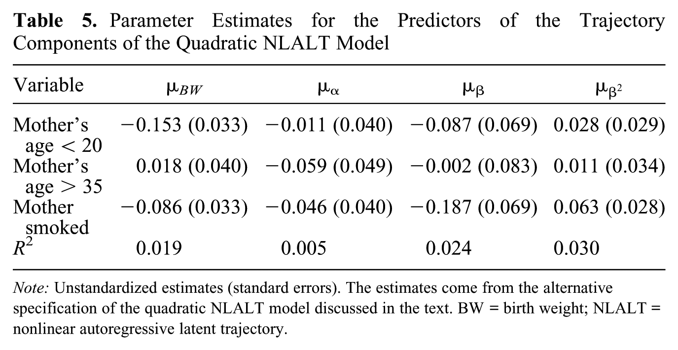
Note: Unstandardized estimates (standard errors). The estimates come from the alternative specification of the quadratic NLALT model discussed in the text. BW = birth weight; NLALT = nonlinear autoregressive latent trajectory.

6. Conclusion

With longitudinal data we rarely a priori know the correct growth model to apply. As such, it is important to rely on substantive knowledge, theory, and data visualization to assess functional form and the potential presence of autoregressive processes. In addition, it is important to have longitudinal models that permit a range of functional forms in combination with an autoregressive component. In this paper, we have generalized the linear ALT model, a flexible growth model that permits both linear case-specific growth curves and autoregressive effects, to accommodate two forms of nonlinear case-specific growth curves: a quadratic NLALT and a latent basis (or freed loading) NLALT. In particular, we provide the parameterization, baseline model identification status, and a treatment of how to test both NLALT models against three more parsimonious longitudinal models. We also illustrate with a simulation study the potential bias in the estimates of the growth parameters that can arise from fitting an incorrect growth model to a set of trajectories based on a nonlinear case-specific component and an autoregressive component.

In addition to expanding the statistical tool kit for modeling longitudinal processes, NLALT models also address a concern with linear ALT models that they may be misspecified when fit to nonlinear trajectories. It is possible for a true model to be a linear ALT model but for researchers to mistakenly fit a quadratic model or for a true model to be a quadratic growth curve model and to fit a linear ALT model. The two NLALT models we have outlined provide a more general structure in which versions of both a linear ALT and a quadratic growth curve model are nested. This nesting permits statistical tests of the presence of an autoregressive process and nonlinear, individual-specific trajectories and thus helps adjudicate between a linear ALT and a nonlinear growth curve model for cases that do not involve both types of processes.

Though the two NLALT models provide additional possibilities for modeling longitudinal data, they also suggest avenues for further research. Earlier in the paper we mentioned that our focus was on autoregressive relations among the repeated measures rather than among the disturbances of the equations. One potentially promising area of development would be to determine whether the ALT and NLALT models could be extended to include both autoregression among the repeated measures as well as among the disturbances. In addition, we have focused on autoregressive processes with a single lag—that is, AR(1)— as these are most relevant for the large-N, small-T data that are typically available for growth curve modeling. Nonetheless, another possible extension would be to consider autoregressive processes for the repeated measures that include additional lag effects—for example, AR(2) or higher models.

Currently there is considerable interest in mixture models for longitudinal data in which there are latent classes within a sample that follow different mean trajectories (e.g., Collins and Lanza 2010). Structural misspecification can create latent classes to compensate for the misspecifications even if a single group underlies the data (Bauer and Curran 2003). It would be valuable to fit a NLALT model to see whether nonlinear or autoregressive relations are present in the data before turning to mixture models with a linear growth curve. It may even be possible to incorporate ALT or NLALT models into a mixture modeling framework that would allow for an assessment of whether latent classes with different ALT or NLALT parameters are present in the data. Finally, we have focused on the two most commonly used nonlinear growth curve model specifications, but there are other inherently nonlinear functions (such as exponential, logistic, or Gompertz functions) that have been considered within an SEM framework (Browne 1993; Browne and du Toit 1991). It would be interesting to explore whether these alternative nonlinear functional forms could also be incorporated into additional types of NLALT models.

Supplemental Material

SM789441_Appendix – Supplemental material for Nonlinear Autoregressive Latent Trajectory Models

Supplemental material, SM789441_Appendix for Nonlinear Autoregressive Latent Trajectory Models by Shawn Bauldry and Kenneth A. Bollen in Sociological Methodology

Footnotes

Authors’ Note

We provide information in the manuscript for how to obtain the data we used in the empirical example.

Notes

Author Biographies

Shawn Bauldry is an assistant professor in the Department of Sociology at Purdue University. His methodological research focuses on the development of structural equation models, including models for longitudinal data, nontraditional measurement models, and instrumental variable estimators.

Kenneth A. Bollen is the Henry Rudolph Immerwahr Distinguished Professor in the Department of Psychology and Neuroscience and Department of Sociology at the University of North Carolina at Chapel Hill. He is a faculty member in the Quantitative Psychology Program in the Thurstone Psychometric Laboratory. He is also chair of the Methods Core and a fellow of the Carolina Population Center and a faculty member of the Center for Developmental Science. Since 1980 he has been an instructor in the ICPSR Summer Program in Quantitative Methods of Social Research at the University of Michigan. His recent research focuses on creating methodological tools applicable to modeling longitudinal and time series data, nontraditional measurement models, and estimators robust to misspecifications. Population and health outcomes provide the substantive contexts for this methodological work. More background information is available at .

References

Adair

Linda S.

Popkin

Barry M.

Akin

John S.

Guilkey

David K.

Gultiano

Socorro

Borja

Judith

Perez

Lorna

Kuzawa

Christopher W.

McDade

Thomas

Hindin

Michelle J.

2011. “Cohort Profile: The Cebu Longitudinal Health and Nutrition Survey.” International Journal of Epidemiology 40:619–25.

Aldous

Michael B.

Edmonson

M. Bruce

. 1993. “Maternal Age at First Childbirth and Risk of Birth Weight and Preterm Delivery in Washington State.” JAMA 270:2574–77.

Arbuckle

James L.

1996. “Full Information Estimation in the Presence of Incomplete Data.” Pp. 243–77 in Advanced Structural Equation Modeling: Issues and Techniques, edited by Marcoulides

G. A.

Schumacker

R. E.

Mahwah, NJ: Lawrence Erlbaum.

Arbuckle

James L.

2006. Amos (Version 7.0) [Computer program]. Chicago: SPSS.

Bast

Janwillem

Reitsma

Pieter

. 1997. “Matthew Effects in Reading: A Comparison of Latent Growth Curve Models and Simplex Models with Structured Means.” Multivariate Behavioral Research 32:135–67.

Bauer

Daniel J.

Curran

Patrick J.

2003. “Distributional Assumptions of Growth Mixtures Models: Implications for Overextraction of Latent Trajectory Classes.” Psychological Methods 11:338–63.

Bentler

Peter

. 1990. “Comparative Fit Indexes in Structural Models.” Psychological Bulletin 107:238–46.

Bianconcini

Silvia

. 2012. “Nonlinear and Quasi-simplex Patterns in Latent Growth Models.” Multivariate Behavioral Research 47:88–114.

Bianconcini

Silvia

Bollen

Kenneth A.

2018. “The Latent Variable–Autoregressive Latent Trajectory (LV-ALT) Model: A General Framework for Longitudinal Data Analysis.” Structural Equation Modeling. Retrieved May15, 2018 (https://www-tandfonline-com-s.web.bisu.edu.cn/doi/abs/10.1080/10705511.2018.1426467?journalCode=hsem20).

10.

Bollen

Kenneth A.

1989. Structural Equations with Latent Variables. New York: Wiley.

11.

Bollen

Kenneth A.

Bauldry

Shawn

. 2010. “Model Identification and Computer Algebra.” Sociological Methods and Research 39:127–56.

12.

Bollen

Kenneth A.

Curran

Patrick J.

1999. “An Autoregressive Latent Trajectory (ALT)Model: A Synthesis of Two Traditions.” Presented at the annual meeting of the Psychometric Society, Lawrence, KS.

13.

Bollen

Kenneth A.

Curran

Patrick J.

2004. “Autoregressive Latent Trajectory (ALT) Models: A Synthesis of Two Traditions.” Sociological Methods and Research 32:336–83.

14.

Bollen

Kenneth A.

Curran

Patrick J.

2006. Latent Curve Models. New York: Wiley.

15.

Bollen

Kenneth A.

Stine

Robert

. 1990. “Direct and Indirect Effects: Classical and Bootstrap Estimates of Variability.” Pp. 115–40 in Sociological Methodology, vol. 20, edited by Clogg

C. C.

Oxford, UK: Basil Blackwell.

16.

Bollen

Kenneth A.

Stine

Robert

. 1993. “Bootstrapping Goodness-of-fit Measures in Structural Equation Models.” Pp. 111–35 in Testing Structural Equation Models, edited by Bollen

K. A.

Long

J. S.

Newbury Park, CA: Sage.

17.

Browne

Michael W.

1984. “Asymptotic Distribution Free Methods in the Analysis of Covariance Structures.” British Journal of Mathematical and Statistical Psychology 37:62–83.

18.

Browne

Michael W.

1993. “Structured Latent Curve Models.” Pp. 171–97 in Multivariate Analysis: Future Directions 2, edited by Cuadras

C. M.

Rao

C. R.

Amsterdam: Elsevier.

19.

Browne

Michael W.

du Toit

Stephen H. C.

1991. “Models for Learning Data.” Pp. 47–68 in Best Methods for the Analysis of Change, edited by Collins

L. M.

Horn

J. L.

Washington, DC: American Psychological Association.

20.

Cameron

A. Colin

Trivedi

Pravin K.

2005. Microeconometrics: Methods and Applications. New York: Cambridge University Press.

21.

Caprara

Gian Vittorio

Eisenberg

Nancy

Allesandri

Guido

. 2017. “Positivity: The Dispositional Basis of Happiness.” Journal of Happiness Studies 18:353–71.

22.

Chi

Eric M.

Reinsel

Gregory C.

1989. “Models for Longitudinal Data with Random Effects and AR(1) Errors.” Journal of the American Statistical Association 84:452–59.

23.

Collins

Linda M.

Lanza

Stephanie T.

2010. Latent Class and Latent Transition Analysis. Hoboken, NJ: Wiley.

24.

Conter

Valentino

Cortinovis

Ivan

Rogari

Patrizia

Riva

Luca

. 1995. “Weight Growth in Infants Born to Mothers Who Smoked During Pregnancy.” BMJ 310:768–71.

25.

Copeland

Molly

Bartlett

Bryce

Fisher

Jacob C.

2017. “Dynamic Associations of Network Isolation and Smoking Behavior.” Network Science 5:257–77.

26.

Curran

Patrick J.

Bollen

Kenneth A.

1999. “Extensions of the Autoregressive Latent Trajectory Model: Explanatory Variables and Multiple Group Analysis.”Presented at the annual meeting of the Society for Prevention Research, New Orleans, LA.

27.

Curran

Patrick J.

Bollen

Kenneth A.

2001. “The Best of Both Worlds: Combining Autoregressive and Latent Curve Models.” Pp. 107–35 in New Methods for the Analysis of Change, edited by Collins

L. M.

Sayer

A. G.

Washington, DC: American Psychological Association.

28.

Diggle

Peter J.

Liang

Kung-Yee

Zeger

Scott L.

1994. Analysis of Longitudinal Data. Oxford, UK: Clarendon Press.

29.

Graff

1979. “Verallgemeinertes LSIREL-Modell.” Unpublished manuscript. Mannheim, Germany.

30.

Graff

Schmidt

1982. “A General Model for Decomposition of Effects.” Pp. 131–48 in Systems under Indirect Observation, edited by Joreskog

K. G.

Wold

H. O. A.

Amsterdam: North-Holland.

31.

Guttman

Louis

. 1954. “A New Approach to Factor Analysis: The Radex.” Pp. 258–348 in Mathematical Thinking in the Social Sciences, edited by Lazarfeld

P. F.

New York: Columbia University Press.

32.

Hamaker

Ellen L.

2005. “Conditions for the Equivalence of the Autoregressive Latent Trajectory Model and a Latent Growth Curve Model with Autoregressive Disturbances.” Sociological Methods and Research 33:404–16.

33.

Heise

David R.

1969. “Separating Reliability and Stability in Test-retest Correlation.” American Sociological Review 34:93–101.

34.

Humphreys

Lloyd G.

1960. “Investigations of the Simplex.” Psychometrika 25:313–23.

35.

Jongerling

Joran

Hamaker

Ellen L.

2011. “On the Trajectories of the Predetermined ALT Model: What Are We Really Modeling.” Structural Equation Modeling 18:370–82.

36.

Jö reskog

Karl G.

1970. “A General Method for Analysis of Covariance Structures.” Biometrika 57:239–51.

37.

Jöreskog

Karl G.

Sorbom

Dag

. 2005. LISREL 8.7 for Windows [Computer software]. Lincolnwood, IL: Scientific Software International.

38.

Kenny

David A.

Campbell

Donald T.

1989. “On the Measurement of Stability in Over-time Data.” Journal of Personality 57:445–81.

39.

Kessler

Ronald C.

Greenberg

David F.

1981. Linear Panel Analysis. New York: Academic Press.

40.

Kolenikov

Stanislav

Bollen

Kenneth A.

2012. “Testing Negative Error Variances: Is a Heywood Case a Symptom of Misspecification?” Sociological Methods and Research 41:124–67.

41.

MapleSoft. 2017. Maple 2017.1 [Computer software]. Waterloo, ON: Waterloo Maple.

42.

McArdle

John J.

1988. “Dynamic but Structural Equation Modeling of Repeated Measures Data.” Pp. 561–614 in The Handbook of Multivariate Experimental Psychology, edited by Nesselroade

J. R.

Cattell

R. B.

New York: Plenum Press.

43.

McArdle

J. Jack

McDonald

Roderick P.

1984. “Some Algebraic Properties of the Reticular Action Model for Moment Structures.” British Journal of Mathematical and Statistical Psychology 37:234–51.

44.

McLaughlin

Katie A.

King

Kevin

. 2015. “Development Trajectories of Anxiety and Depression in Early Adolescence.” Journal of Abnormal Child Psychology 43:311–23.

45.

Meredith

William

Tisak

John

. 1984. “‘Tuckerizing’ Curves.”Presented at the annual meeting of the Psychometric Society, Santa Barbara, CA.

46.

Meredith

William

Tisak

John

. 1990. “Latent Curve Analysis.” Psychometrika 55:107–22.

47.

Muthén

Linda K.

Muthén

Bengt

. 2012. Mplus User’s Guide. Los Angeles: Muthén and Muthén.

48.

Chow

Sy-Miin

Linying

Molenaar

Peter C. M.

2017. “(Re)evaluating the Implications of the Autoregressive Latent Trajectory Model through Likelihood Ratio Tests of Its Initial Conditions.” Multivariate Behavioral Research 52:178–99.

49.

Parker

Philip D.

Marsh

Herbert W.

Morin

Alexandre J. S.

Seaton

Marjorie

Van Zanden

Brooke

. 2015. “If One Goes Up the Other Must Come Down: Examining Ipsative Relationships between Math and English Self-concept Trajectories across High School.” British Journal of Educational Psychology 85:172–91.

50.

Raftery

Adrian

. 1995. “Bayesian Model Selection in Social Research.” Pp. 111–63 in Sociological Methodology, vol. 25, edited by Marsden

P. V.

Oxford, UK: Blackwell.

51.

Rao

C. R.

1958. “Some Statistical Methods for Comparison of Growth Curves.” Biometrika 51:83–90.

52.

Rogosa

David R.

Brandt

David

Zimowski

Michele

. 1982. “A Growth Curve Approach to the Measurement of Change.” Psychological Bulletin 92:726–48.

53.

Rogosa

David R.

Willett

John B.

1985. “Satisfying Simplex Structure Is Simpler Than It Should Be.” Journal of Educational Statistics 10:99–107.

54.

Rosseel

Yves

. 2012. “Lavaan: An R Package for Structural Equation Modeling.” Journal of Statistical Software 48:1–36.

55.

Rothenberg

Thomas J.

1971. “Identification in Parametric Models.” Econometrica 39:577–91.

56.

Satorra

Albert

. 1990. “Robustness Issues in Structural Equation Modeling: A Review of Recent Developments.” Quality and Quantity 24:367–86.

57.

Schwarz

Gideon

. 1978. “Estimating the Dimension of a Model.” Annals of Statistics 6:461–64.

58.

Smith

Justin D.

Dishion

Thomas J.

Shaw

Daniel S.

Wilson

Melvin N.

Winter

Charlotte C.

Patterson

Gerald R.

2014. “Coercive Family Process and Early-onset Conduct Problems from Age 2 to School Entry.” Development and Psychopathology 26:917–32.

59.

StataCorp. 2017. Stata Statistical Software: Release 15. College Station, TX: StataCorp LP.

60.

Steiger

James H.

Lind

John C.

1980. “Statistically-based Tests for the Number of Common Factors.”Presented at the annual meeting of the Psychometric Society, Iowa City, IA.

61.

Tucker

Ledyard R.

1958. “Determination of Parameters of a Functional Relation by Factor Analysis.” Psychometrika 23:19–23.

62.

Tucker

Ledyard R.

Lewis

Charles

. 1973. “A Reliability Coefficient for Maximum Likelihood Factor Analysis.” Psychometrika 38:1–10.

63.

Voelkle

Manuel C.

2008. “Reconsidering the Use of Autoregressive Latent Trajectory (ALT) Models.” Multivariate Behavioral Research 43:564–91.

64.

Werts

Charles E.

Jöreskog

Karl G.

Linn

Robert L.

1971. “Comment on ‘The Estimation of Measurement Error in Panel Data.’” American Sociological Review 36:110–13.

65.

WHO Multicentre Growth Reference Study Group. 2006. “WHO Child Growth Standards Based on Length/Height, Weight, and Age.” Acta Paediatrica 450:76–85.

66.

Wiley

David E.

Wiley

James A.

1970. “The Estimation of Measurement Error in Panel Data.” American Sociological Review 35:112–17.

Supplementary Material

Please find the following supplemental material available below.

For Open Access articles published under a Creative Commons License, all supplemental material carries the same license as the article it is associated with.

For non-Open Access articles published, all supplemental material carries a non-exclusive license, and permission requests for re-use of supplemental material or any part of supplemental material shall be sent directly to the copyright owner as specified in the copyright notice associated with the article.

0.00 MB

0.02 MB