The Spatial Proximity and Connectivity Method for Measuring and Analyzing Residential Segregation

Abstract

In recent years, there has been increasing attention focused on the spatial dimensions of residential segregation—from the spatial arrangement of segregated neighborhoods to the geographic scale or relative size of segregated areas. However, the methods used to measure segregation do not incorporate features of the built environment, such as the road connectivity between locations or the physical barriers that divide groups. This paper introduces the spatial proximity and connectivity (SPC) method for measuring and analyzing segregation. The method addresses the limitations of current approaches by taking into account how the physical structure of the built environment affects the proximity and connectivity of locations. I describe the method and its application for studying segregation and spatial inequality more broadly, and I demonstrate one such application—analyzing the impact of physical barriers on residential segregation—with a stylized example and an empirical analysis of racial segregation in Pittsburgh, Pennsylvania. The SPC method contributes to scholarship on residential segregation by capturing the effect of an important yet understudied mechanism of segregation—the connectivity, or physical barriers, between locations—on the level and spatial pattern of segregation, and it enables further consideration of the role of the built environment in segregation processes.

Keywords

segregation measurement boundaries spatial analysis built environment

1. Introduction

Over the past century, scholars have generated a cumulative body of knowledge on the prevalence, causes, and consequences of residential segregation, and they have established segregation as a key mechanism of social stratification (for a review, see Charles 2003; see also Bruch 2014; Logan 2013; Massey 2016; Massey and Denton 1993; Quillian 2012; Sampson and Sharkey 2008). In recent years, there has been increasing recognition that popular summary indexes of segregation, such as the dissimilarity index, allow researchers to describe certain characteristics of residential segregation but fail to capture differences in the spatial organization of segregation patterns, such as the spatial arrangement of segregated neighborhoods and the geographic scale or relative size of segregated areas (Brown and Chung 2006; Morrill 1991; Reardon and O’Sullivan 2004; White 1983). Consequently, more attention has been paid to the spatial dimensions of residential segregation, with newly developed methods and an increasing number of studies on the topic (e.g., Bischoff 2008; Chodrow 2017; Crowder and South 2008; Farrell 2008; Fischer 2008; Fischer et al. 2004; Folch and Rey 2016; Fowler 2015; Grannis 1998; Grigoryeva and Ruef 2015; Lee et al. 2008; Lichter, Parisi, and Taquino 2015; Logan 2017; O’Sullivan and Wong 2007; Reardon and Bischoff 2011; Reardon et al. 2009; Spielman and Logan 2013; Xu, Logan, and Short 2014).

Although these developments have undoubtedly advanced our understanding of segregation, the newly developed methods do not incorporate features of the built environment—including the physical barriers that divide cities and reduce connectivity between nearby areas—into the measurement of segregation. Physical barriers such as highways and railroad tracks influence residential sorting processes by providing clear divisions between areas and yielding agreement among residents, real estate agents, and other institutional actors about where one neighborhood ends and another begins (Ananat 2011; Bader and Krysan 2015). They ease the categorization of areas in the housing search process (Bader and Krysan 2015; Krysan and Bader 2009) and purport to offer “protection” from residents on the other side of a boundary (Atkinson and Flint 2004; Blakely and Snyder 1997; Low 2001; Schindler 2015). As a result, the presence of these barriers can create distinct social conditions and experiences for individuals on different sides of them, as exemplified by the common metaphor “the other side of the tracks.”

Spatial features such as streets or landmarks can carry symbolic meaning as a border between residents of different groups (Kramer 2017) and structure residential preferences and discrimination (Besbris et al. 2015). However, these features are still fluid and negotiable and offer the possibility for integration (Anderson 1990; Hunter 1974; Hwang 2016; Suttles 1972). In contrast, physical barriers are strong and persistent forms of boundaries that limit physical connectivity between areas and require institutional action, such as urban planning and infrastructure investment, to dismantle (Jackson 1985; Mohl 2002; Schindler 2015). Moreover, some physical barriers were originally constructed with an intention to racially segregate nearby populations (Mohl 2002; Schindler 2015; Sugrue 2005)—a notable example being the selection of routes for interstate highways built during the 1950s and 1960s in cities such as Chicago and Atlanta (Mohl 2002).

This paper introduces a new method for measuring and analyzing segregation: the spatial proximity and connectivity (SPC) method. The method addresses the limitations of current approaches by integrating features of the built environment into the measurement of segregation and analyzing the level and spatial pattern of segregation revealed by such measures. My proposed approach contributes to the scholarship on residential segregation by capturing the effect of an important yet understudied mechanism of segregation—the connectivity, or physical barriers, between locations—and it enables further consideration of the role of the built environment in segregation processes.

Section 2 reviews current spatial approaches for measuring residential segregation and discusses their limitations. Section 3 introduces the SPC method and describes each of its six steps. Section 4 outlines a wide range of applications relevant to studying segregation and spatial inequality more broadly. Section 4.1 demonstrates one such application—measuring the impact of physical barriers on residential segregation—using a stylized example and an empirical case. Section 4.1.1 examines a stylized city with a north-south pattern of segregation similar to the patterns of white-black segregation in St. Louis or Cleveland. I introduce various physical barriers into the city and compare how segregation changes when each type of barrier is present. Section 4.1.2 examines patterns of racial segregation in Pittsburgh. I compare segregation measures that do and do not take into account the road connectivity between locations, and I evaluate the extent to which physical barriers facilitate greater separation between groups and are associated with higher levels of local and citywide segregation. Section 5 summarizes the contribution of the SPC method and discusses possible applications and extensions of the method for future research.

2. Measuring Residential Segregation

Scholars have engaged in a longstanding debate about how best to measure residential segregation (for a brief history, see Reardon and Firebaugh 2002). The dissimilarity index came into widespread use in the mid–twentieth century and remains the most popular measure of segregation. Although summary indexes such as this one allow researchers to describe distributional characteristics of residential segregation (Massey and Denton 1988), they are “aspatial”—they do not integrate the fundamentally spatial concepts of proximity and geographic scale into the measurement of segregation. Spatial proximity concerns the location of areas relative to one another, such as how neighborhoods are spatially arranged in a city. Geographic scale concerns the relative size of segregated clusters or geographic extent of segregation patterns.

The shortcomings of aspatial approaches are summarized by two well-documented methodological problems: the checkerboard problem and the modifiable areal unit problem (MAUP). The checkerboard problem (Duncan and Duncan 1955; Taeuber and Taeuber 1965; White 1983) describes the failure of aspatial approaches to account for the arrangement or relative position of spatial units. If we imagine the squares on a checkerboard to be neighborhoods with a given composition, there are many possible ways the neighborhoods can be arranged to create different spatial patterns of segregation. But, if we do not take into account where they are located relative to one another, any arrangement of the neighborhoods would result in the same segregation score. The MAUP occurs when the composition of spatial units is affected by changes to the boundaries, number, or size of the spatial units (Fotheringham and Wong 1991; Openshaw 1984; Openshaw and Taylor 1979). This is problematic if the spatial units are defined by arbitrary boundaries rather than being socially meaningful entities (Bischoff 2008; Reardon and O’Sullivan 2004; Xu et al. 2014).

Several spatial approaches for measuring segregation have addressed these concerns, which I organize into three types of strategies: (1) comparing nested levels of geography, (2) identifying spatial neighbors, and (3) constructing egocentric neighborhoods. In the remainder of this section, I briefly describe each of these strategies and summarize the problems that they solve and those that remain.

2.1. Comparing Nested Levels of Geography

First, a popular strategy for addressing the checkerboard problem is to analyze the geographic scale of segregation patterns by comparing segregation within or between nested levels of geography. Studies have measured segregation for increasingly large units of geography, such as census tracts nested in municipalities within a metropolitan area, and compared the segregation occurring at each level. For example, Massey, Rothwell, and Domina (2009) measure segregation with the dissimilarity index and find that declines in black-white segregation have occurred primarily at the tract level, with very little change in the segregation level of cities, counties, or states since 1970. However, using this approach, we cannot compare how much the segregation for each level of geography contributes to the overall level of segregation in the region.

Another approach is to use a measure that allows us to decompose the overall segregation in a region into the segregation occurring within and between places in the region and then compare the contribution of micro (i.e., within each place) and macro (i.e., between places) segregation components with overall segregation. Several recent studies have used Theil’s entropy index for decompositions within and between the cities and suburbs of U.S. metropolitan areas (Farrell 2008; Fischer 2008; Fischer et al. 2004; Fowler, Lee, and Matthews 2016; Lichter et al. 2015; Parisi, Lichter, and Taquino 2011). Although Theil’s entropy index is a measure of diversity, not segregation—it compares the diversity of smaller spatial units relative to the larger aggregate area rather than comparing their compositions¹—this approach could be adapted to use a decomposable measure of segregation, such as the divergence index (Roberto 2016).² A decomposition approach allows us to compare the contributions of each level of geography with overall segregation (or diversity); however, it does not account for differences in the spatial arrangement of geographic units within each level.

2.2. Identifying Spatial Neighbors

A second strategy for addressing the checkerboard problem is to integrate information about the relative proximity of neighborhoods (e.g., census tracts) when measuring segregation. This is typically done in one of two ways: either by identifying adjacent neighborhoods (i.e., immediate neighbors that share a boundary, neighborhoods that have a common neighbor, etc.) or calculating the geographic distance between the center point of each pair of neighborhoods. Several spatial indexes have been developed to accommodate information about proximity when measuring segregation (for a review, see Reardon and O’Sullivan 2004). They typically use a proximity function to incorporate the population of nearby areas into each neighborhood’s population composition, with a weight that determines the relative contribution of distant versus nearby areas. For example, a uniform (or rectangular) proximity function gives equal weight to distant and nearby areas as long as they are within a given distance band (e.g., Jargowsky and Kim 2005; Wu and Sui 2001), or a distance-decay function can be used to weight nearby areas more heavily than distant areas, with the rate of decay intended to represent the influence of distance on social interaction patterns (White 1983). Although this strategy accounts for the spatial arrangement of neighborhoods, it still relies on census units, such as tracts, which vary in geographic size and population density across the country.

2.3. Constructing Egocentric Neighborhoods

In contrast to conventional approaches that use census tracts to measure segregation, a third strategy uses “egocentric neighborhoods” to measure segregation and addresses both the checkerboard problem and MAUP. For example, Reardon and colleagues (Lee et al. 2008; Reardon et al. 2008, 2009) superimpose a grid with 50 by 50 meter cells over the census blocks of a metropolitan area and estimate the population in each cell.³ They then measure the shortest straight line distance between the center points of all pairs of cells and use these distances to construct local environments, or “egocentric neighborhoods,” around each of the cells. The local environment of each cell includes nearby cells within a particular distance, and they systematically vary the distance using radii of .5, 1, 2, and 4 km (.3, .6, 1.2, and 2.5 miles). They use a proximity function that weights the share of the population of nearby cells that will be included in a cell’s local environment.⁴ They measure segregation separately for local environments constructed with each radius and compare changes in the level of segregation as the radius increases.

By dispensing with census tracts in favor of egocentric neighborhoods of various sizes, this approach is able to distinguish between the geographic scale and methodological scale of segregation—between the scale at which segregation is experienced in social environments and the level of aggregation in the data (Reardon et al. 2008). Although this is a large step forward for spatial segregation measurement, a notable limitation remains: The method does not integrate features of the built environment into the measurement of distance. Specifically, by using the straight line distance between grid cells to measure proximity, the approach ignores the physical barriers that divide urban space and the connectivity provided by roads. It is therefore unable to detect any difference in segregation whether nearby areas are separated by a physical barrier, such as a fence, railroad tracks, or dead-end streets, or if they are well connected by roads.

3. The Spatial Proximity and Connectivity Method

I propose a new method for measuring and analyzing segregation: the spatial proximity and connectivity method (SPC). Consistent with recent advancements in segregation measurement, SPC addresses the checkerboard problem and MAUP by measuring spatial proximity and comparing segregation at multiple geographic scales.⁵ However, the SPC method also addresses the limitations of previous approaches by using a realistic measure of distance that integrates information about the built environment.

Existing methods that use distance to measure spatial proximity rely on straight line distance—the shortest distance from Point A to Point B—without considering that spatial areas are often connected not by straight lines but rather by a road network. In contrast, SPC measures the shortest distance between all residential locations along a city’s road network, which reflects the connectivity between locations and the separation imposed by physical barriers. This is an important feature of SPC because two residential areas may be spatially proximate to each other but not well connected by roads (Neal 2012). For example, in a study of racial settlement patterns in Los Angeles and San Francisco, Grannis (1998) found that connectivity along small residential streets was more important than mere proximity in predicting racial segregation patterns.

Physical barriers have also been used as mechanisms to reinforce or exacerbate segregation by facilitating greater separation between ethnoracial groups in nearby areas. For example, Jackson (1985) describes adjacent black and white neighborhoods in the vicinity of Eight Mile Road in Detroit in the late 1930s. None of the white families could get Federal Housing Administration (FHA) mortgages “because of the proximity of an ‘inharmonious’ racial group” (Jackson 1985:209). After a developer built a concrete wall between the neighborhoods in 1941, FHA approved mortgages for properties in the white neighborhood. The SPC method contributes to the scholarship on residential segregation by capturing the effect of this additional mechanism of segregation—the connectivity, or physical barriers, between locations—on the level and pattern of segregation.

Sections 3.1 to 3.6 describe each step of the SPC method. Using road distance to measure the proximity and connectivity between locations requires six steps: (1) linking the geographic data for blocks and roads, (2) estimating the population count and composition at locations on the road network, (3) calculating the distance of the shortest path between all locations, (4) constructing local environments around each location, (5) calculating proximity weights, and (6) measuring segregation.

For each of these steps, I use R software (R Core Team 2014) and add-on packages designed for working with spatial data (Bivand, Keitt, and Rowlingson 2017; Bivand and Rundel 2017; Neuwirth 2014; Pebesma and Bivand 2005), networks (Csardi and Nepusz 2006), and large matrices (Kane, Emerson, and Weston 2013; Revolution Analytics and Weston 2014). Although my explanation focuses on using the SPC approach to study residential segregation in cities, the method is applicable to any area of interest (e.g., school districts, metropolitan areas, and states), including rural areas.

3.1. Step 1: Linking the Geographic Data

SPC uses publicly available population data from the 2010 decennial census (U.S. Census Bureau 2011) and the geographic data provided in TIGER/Line shapefiles (U.S. Census Bureau 2012). The U.S. census subdivides the entire United States into several nested geographic units. I use population data for census blocks—the smallest unit of census geography. Blocks are polygons that are typically bounded by street or road segments on each side and typically correspond to a residential city block in urban areas. Blocks can also represent spatial areas without population or nonresidential land use, such as industrial areas, parks, or areas between railroad tracks. Blocks are nested within census tracts—the most commonly used unit of census geography for measuring segregation—which contain an average population of 4,000 individuals.

SPC uses the TIGER/Line shapefiles for “faces” and “edges” to define the geographic boundaries of blocks and the path of roads. Faces are polygons that represent area features, such as blocks. Each face is assigned a permanent unique identifier (UID) by the Census Bureau. A block usually consists of a single face, but in some cases, a block may contain two or more faces (e.g., if an alley subdivides a block). Each face is bounded by one or more edges. Edges are line features, including road segments, and each edge has a UID. Each edge is associated with two faces—one on each of its sides. The two endpoints of an edge are called nodes, and each has a UID. A single node may be associated with multiple edges, such as a node that joins together two road segments.

For example, Figure 1 shows two blocks, the seven road segments that define their perimeters, and the intersections of the roads. Each of the blocks has one face, each with a UID. Each road segment has an edge UID, and each endpoint of a road has a node UID. Roads that intersect have nodes in common. For example, node 65970117 in Figure 1 is an endpoint of edges 3701349, 3701194, and 3701350. This node is the shared intersection of Center St. and the two segments of Church St.

Figure 1.

An example of the TIGER/Line features used to construct road networks.

I use the UIDs to link the geographic data for each city by identifying the relationships between blocks, faces, edges, and nodes. The data record for each face includes its UID, and if it represents a block feature, then it includes the UID for the block. The data record for each edge includes the edge’s UID, the two node UIDs for its endpoints, and the two face UIDs for its sides. The record also indicates whether the edge is a road feature; if it is, it provides a classification code for the type of road feature (primary road, local road, alley, etc.). For each block, I identify the face UIDs associated with the block, find the UID for any roads features (including alleys and pedestrian walkways) that have the block’s face UIDs listed as one of its sides, and collect all of the node UIDs associated with those roads. The result is a list of the road UIDs and node UIDs associated with each block.

3.2. Step 2: Estimating the Population Count and Composition of Nodes

Once the geographic data for blocks, roads, and nodes have been linked, I estimate the population count and composition at each of the nodes.⁶ This procedure distributes the aggregate population of each block to point locations on roads by assigning a portion of each block’s population to the nodes associated with the block.⁷ In step 5 (Section 3.5), this will allow us to calculate the population composition in the local environment around each node. It also has the advantage of removing the arbitrary administrative boundaries of individual census blocks, and it smoothes the distribution of the population and sharp discontinuities that may occur along the administrative boundaries.⁸

I assign the block’s population to the nodes in two stages. First, I assign individuals to one of the roads associated with the block, with the probability of assignment equal to the length of the road segment. Second, I randomly assign individuals to one of the two nodes that are the endpoints of their assigned road segment. When adjacent blocks are associated with the same node, such as node 65970117 in Figure 1, the node will likely receive a portion of each block’s population.

The random assignment of block populations to nodes will affect the population count and composition of each node. The randomness of the procedure would likely affect segregation levels if each node was a unit of analysis, as with aspatial segregation measures. However, in the fourth step (Section 3.4), SPC measures segregation in the local environment around each node, which incorporates the population of nearby nodes into the local environment’s composition. Even at a reach of 0 km, much of the variability of random assignment is mitigated because adjacent blocks share nodes and each block contributes to the node’s population. To err on the side of caution, the size of local environments should be at least as large as the typical census block in a given city, in which case, variability in the population count or composition due to sampling is likely to be minimal.

3.3. Step 3: Calculating the Shortest Paths

Step 3 of the SPC method calculates the shortest paths between all pairs of nodes. The length of the shortest paths is the minimum road distance between nodes. I measure the shortest paths by first constructing a graph that represents the road network. SPC takes advantage of the relational nature of the geographic data to construct the graph. The edgelist of the graph contains each road segment as an edge and its endpoints—the nodes—as the vertices. A single node can join multiple road segments, which provides the necessary linkages to construct the network. The record for each edge includes the UID for the road segment (i.e., the edge), the UIDs for the nodes at its endpoints (i.e., the vertices), and the length of the road segment (i.e., the edge weight). The graph is undirected, meaning that if vertex A is connected to vertex B, then vertex B is also connected to vertex A.⁹ The weight of the edge connecting vertex A and vertex B represents the road distance between them. Once the graph is constructed, I calculate the length of the shortest path between each pair of nodes in the network using the Dijkstra algorithm implemented in the igraph package for R (Csardi and Nepusz 2006).

3.4. Step 4: Constructing Local Environments

I use the egocentric neighborhoods strategy described in Section 2.3 to construct local environments around each node, systematically vary their size, and record the population composition within all local environments of each size (e.g., Lee et al. 2008). However, I define the size, or reach (i.e., the distance in each direction from a given node), of local environments using the road network distance rather than the straight line distance. I systematically vary the reach of local environments within a range of values, such as .1 to 10 km (.06 to 6.2 miles). Local environments with a reach of .1 km are about the size of a block in many cities, whereas local environments with a reach of 10 km encompass a substantial portion of all but the largest U.S. cities. Local environments can span bodies of water, such as rivers and lakes, and will include the population on the other side of the water if it is within the reach.

When using local environments, a choice must be made about whether locations near the boundary of the study region will be constrained to be within the boundary or extend into areas outside the region. For example, will the local environment of a node near the boundary of a city include the population of nodes outside the city that are within the given reach of the node? This decision is particularly important if the population composition differs inside the region and in nearby areas outside the region and the region is defined by an arbitrary boundary rather than being a socially meaningful entity. I explain the options for constructing local environments in greater detail in online Appendix A, along with the advantages and limitations of each option.

Previous studies have used local environments that are truncated at the boundary of the study region (e.g., a city or metropolitan area) and include only those nodes that are within the region (Hipp and Boessen 2013; Lee et al. 2008; Reardon and Bischoff 2011; Reardon et al. 2008, 2009; Xu et al. 2014). In the steps of the SPC method and the applications that follow, I likewise describe using truncated local environments; however, the method is almost identical when using extended local environments (the exceptions are noted in online Appendix A).

3.5. Step 5: Calculating Proximity Weights

I use a proximity function to weight the relative contribution of distant versus nearby nodes in the population of each node’s local environment. The functional form of the weights should represent a given study’s definition of spatial proximity—for example, by representing patterns of social interaction (e.g., Reardon et al. 2008; Xu et al. 2014) or activity spaces (e.g., Schnell and Yoav 2001; Wong and Shaw 2011)—and it should allow for a theoretically meaningful interpretation of results. Studies commonly use a uniform proximity function or a distance-decay proximity function to calculate the proximity weights.

A uniform (or rectangular) proximity function (e.g., Jargowsky and Kim 2005; Wu and Sui 2001) gives a weight of 1 to all nodes that are within the reach of a node’s local environment and a weight of 0 to nodes that are outside the reach of the local environment. The uniform proximity function is calculated as

ϕ_{r} (i, j) = {\begin{matrix} 1 & if d (i, j) \leq r \\ 0 & otherwise \end{matrix},

(1)

where $d (i, j)$ is the pairwise distance between nodes $i$ and $j$ , and $r$ is the reach of local environments.

A distance-decay function generates weights that vary among the nodes included within node $i$ ’s local environment (White 1983). The weights depend on each node’s distance to node $i$ , where the maximum weight is 1 and the weights approach 0 for nodes within the local environment but at greater distances from $i$ . As with the uniform proximity function, nodes that are outside the reach of the local environment receive a weight of 0. A popular distance-decay function is the two-dimensional biweight kernel proximity function (e.g., Lee et al. 2008; Reardon et al. 2008, 2009), which is calculated as

ϕ_{r} (i, j) = {\begin{matrix} {[\begin{matrix} 1 - {(\frac{d (i, j)}{r})}^{2} \end{matrix}]}^{2} & if d (i, j) \leq r \\ 0 & otherwise \end{matrix} .

(2)

It is often reasonable to assume that nearby locations have a stronger influence on a residential environment than more distant locations, but as Logan, Zhang, and Xu (2010:15) note, “we rarely have enough information or theory to specify more clearly the functional form of this decline.” The question of whether proximity should be measured with a distance threshold function (as with a uniform proximity function), distance-decay function, or another functional form will vary depending on the aims of a study. I suggest using a uniform proximity function when the aim of a study is comparative—for example, varying the reach of local environments (or the measure of distance) and comparing the levels of segregation. Its simple functional form allows for a direct investigation of how differences (or similarities) in composition are related to distance. In studies where this relationship is known or theorized, other functional forms, such as distance-decay, may be more appropriate. (Online Appendix B describes this choice and the differences between the functional forms in greater detail.)

The selected proximity function is then used to calculate the proximity weighted population count and composition in each node’s local environment for each reach.¹⁰ The proximity-weighted population count of each group in the local environment is calculated as

{\tilde{τ}}_{rim} = \int_{j \in R} τ_{jm} ϕ_{r} (i, j) dj,

(3)

where $τ_{jm}$ is the group-specific population count for each node $j$ in region $R$ and $ϕ_{r} (i, j)$ is the pairwise proximity weight for nodes $i$ and $j$ . The total proximity-weighted population count in the local environment is calculated as

{\tilde{τ}}_{ri} = \int_{j \in R} τ_{j} ϕ_{r} (i, j) dj,

(4)

or simply as the sum of ${\tilde{τ}}_{rim}$ across groups ( $m$ ): ${\tilde{τ}}_{ri} = \sum_{m} {\tilde{τ}}_{rim}$ . The proximity weighted population composition for node $i$ is calculated by dividing the proximity weighted population count of each group in $i$ ’s local environment and ${\tilde{τ}}_{rim}$ by the total proximity-weighted population count in the local environment, ${\tilde{τ}}_{ri}$ :

{\tilde{π}}_{rim} = \frac{{\tilde{τ}}_{rim}}{{\tilde{τ}}_{ri}} .

(5)

The value of ${\tilde{π}}_{rim}$ represents the population composition experienced by the residents of node $i$ in their local environment with a reach of $r$ , where the populations of other nodes ( $j$ ) are weighted according to the proximity function $ϕ_{r} (i, j)$ .

3.6. Step 6: Measuring Segregation

I use the proximity-weighted population composition to measure segregation in each local environment and the city as a whole. I measure segregation with the divergence index (Roberto 2016), which measures the difference between the population composition of each local environment and the city’s overall composition. This index measures the same concept of segregation as the dissimilarity index, but it has several advantages. For example, the divergence index can be calculated for both continuous and discrete distributions as well as joint distributions, such as income by race, and it can be decomposed to analyze how much of the overall segregation in a city occurs within versus between population groups or spatial areas.¹¹

The divergence index is based on relative entropy—an information theoretic measure also known as Kullback-Leibler (KL) divergence (Cover and Thomas 2006; Kullback 1987).¹² The values of the divergence index represent how surprising the composition of a local environment is given the overall population composition of the city. The divergence index equals 0—its minimum value—when there is no difference between the local and overall population composition, whereas greater differences produce higher values and indicate a greater degree of segregation. Local values of the divergence index will reach their maximum value when the smallest group in a city is 100 percent of the local population.

I measure segregation with the divergence index to capture the differences between the local and overall proportions of each group. The divergence index for location (i.e., node) $i$ ’s local environment with a reach of $r$ km is

{\tilde{D}}_{ri} = \sum_{m} {\tilde{π}}_{rim} \log \frac{{\tilde{π}}_{rim}}{π_{m}},

(6)

where $π_{m}$ is group $m$ ’s proportion of the region’s (e.g., a city’s) overall population and ${\tilde{π}}_{rim}$ is group $m$ ’s proportion of the proximity-weighted population in location $i$ ’s local environment with reach $r$ .¹³

A region’s overall segregation for a given reach of local environments is the population-weighted mean of the divergence index for all locations, calculated as

{\tilde{D}}_{r} = \sum_{i} \frac{τ_{i}}{T} {\tilde{D}}_{ri},

(7)

where $T$ is the region’s overall population count and $τ_{i}$ is the population count in location $i$ . If all local environments have the same composition as the region’s overall population, then ${\tilde{D}}_{r}$ equals 0, indicating no segregation. More divergence between overall and local proportions indicates more segregation.

The divergence index can also be used to calculate group-specific segregation results. For each reach of local environments, the average degree of segregation experienced by each group is calculated as

{\tilde{D}}_{rm} = \sum_{i} \frac{τ_{im}}{τ_{m}} {\tilde{D}}_{ri},

(8)

where $τ_{m}$ is the region’s overall population of group $m$ and $τ_{im}$ is the population of group $m$ in location $i$ . The weighted mean of the group-specific segregation results is equal to the region’s overall segregation:

{\tilde{D}}_{r} = \sum_{m} \frac{τ_{m}}{T} {\tilde{D}}_{rm} .

(9)

4. Applications of the SPC Method

The SPC method can be applied in a variety of ways to study segregation or spatial inequality more broadly. It can measure residential segregation in cities or any other municipal divisions of interest, such as metropolitan areas or school districts. Or it can be used to compare segregation in the vicinity of public institutions (e.g., libraries) and recreational spaces (e.g., parks) and evaluate the potential for these places and spaces to bring together a representative mix of the city’s population. The method can also measure segregation in the vicinity of environmental hazards (e.g., hazardous waste sites) to evaluate the extent to which particular groups are disproportionately exposed to these risks. Additional data about crime, health, or other population or environmental characteristics can also be incorporated into the SPC method to measure and analyze the segregation or spatial inequality of multiple spatial attributes.

SPC can be used as a replacement for current methods of measuring segregation, or it can be used alongside straight line distance segregation measures to evaluate how segregation levels differ when road connectivity and physical barriers are taken into account. Section 4.1 describes the latter application of the method and provides two demonstrations. Section 4.1.1 compares how segregation differs in a stylized city when various types of physical barriers spatially separate two groups. Section 4.1.2 provides an empirical application that examines the local and city-wide levels of racial segregation in Pittsburgh.

4.1. Measuring the Impact of Physical Barriers on Residential Segregation

Physical barriers are material structures—such as highways and rivers—that reduce the connectivity between locations on either side of the barrier. Features of a city’s street design can act as physical barriers: dead-end streets and culs-de-sac create excess distance between locations, whereas a regular street grid provides greater connectivity between locations. The Dan Ryan Expressway in Chicago’s South Side is a classic example of a physical barrier. It was constructed in the 1960s and separated the white and black residents on either side of the highway (Mohl 2002). Using straight line distance to measure the proximity of these communities would represent their nearness but not their disconnection. Their distance apart would be measured as the width of the highway—the same distance that would exist if the highway were never constructed. Using road network distance more accurately represents the highway as a source of separation: It is a physical barrier that divides the communities and facilitates racial segregation, not residential integration.

The difference between the road distance and the straight line distance between two locations reveals the extent to which road connectivity is limited or physical barriers are present between locations. The road distance between any two locations is always equal to or greater than the straight line distance between them. In a city with a regular street grid with diagonal avenues at every intersection, there would be no difference between the two distance measurements. Even without diagonal avenues, there would still be very little difference between the two distance measurements, especially for relatively nearby locations. If the road network is less connected or there are other types of physical barriers present, the road distance between locations will be greater than their straight line distance. For example, the presence of a dead-end street or cul-de-sac can affect the road distance between nodes in the area, but it will have no effect on the straight line distance between the nodes.

To evaluate the impact of connectivity and physical barriers on local and overall levels of segregation, I compare segregation measures that use straight line distance and road network distance. Following the steps of the SPC method, I construct local environments for every node in a city. However, I define the reach of local environments in two ways: using straight line distance and road distance. In both cases, I systematically vary the reach of local environments from .1 to 10 km (.06 to 6.2 miles). The presence of physical barriers will affect the locations included in the local environments constructed with road distance, not those constructed with straight line distance. Therefore, a greater prevalence of physical barriers will result in a greater difference between the locations included in a local environment constructed with road distance and the locations included in a local environment constructed with straight line distance and potentially a difference in their population compositions.

If roads connect all nodes, then the local environments constructed with each distance measure would be identical in size. The biggest differences will occur in areas where one or more nodes are not well connected to other nearby nodes. For example, if railroad tracks create a physical barrier between nearby areas, they would affect the areas included in each node’s local environment when they are constructed with road distance. Figure 2 illustrates the difference between a local environment constructed with straight line distance and a local environment constructed with road distance for one node located near railroad tracks. Figure 2a shows the node’s local environment constructed with straight line distance: All nodes within .5 km are included in the node’s local environment. Figure 2b shows the node’s local environment constructed with road network distance. The railroad tracts limit the connectivity to areas west of the tracks and severely reduce the number of nodes that are included in the local environment.

Figure 2.

Comparing a local environment constructed with straight line distance and road network distance (reach of the local environment = .5 km). (a) Local environment constructed with straight line distance. (b) Local environment constructed with road network distance.

The presence of physical barriers or disconnected roads is not sufficient to influence segregation levels. For barriers to facilitate higher levels of segregation, they must create greater separation between areas with different population compositions. To make this assessment, I record the population composition within all local environments constructed with each type of distance for each reach, and I measure the segregation of all local environments using the divergence index (Roberto 2016), as described in Section 3. For each reach, I measure segregation separately for the local environments constructed with each type of distance.

If there are no physical barriers between locations and roads are well connected, the local environments constructed with straight line distance and those constructed with road distance will encompass the same areas and have the same composition. There will be no difference in the level of segregation for local environments of a given reach constructed with each type of distance.

If physical barriers are present in an area but there is no difference between the road distance and straight line distance segregation measures for the nodes in that area, this indicates that the racial compositions of their local environments measured by each type of distance are identical and physical barriers do not structure the spatial pattern of segregation in that area. If the road distance segregation measure for a local environment is lower than the straight line distance segregation measure, this indicates that the local environment is in an area with a composition that is similar to the city (i.e., lower segregation) and a physical barrier separates it from an area with a composition that differs from the city (i.e., higher segregation).

If the road distance segregation measure for a local environment is higher than the straight line distance segregation measure, this indicates that physical barriers and disconnectivity play a role in spatially structuring segregation patterns. The greater the difference, the greater the extent to which barriers divide groups and facilitate segregation. These differences may be greater for certain reaches of local environments than others, which would indicate that barriers play a larger role in structuring segregation patterns at some geographic scales than at others.

4.1.1. Physical Barriers and Racial Segregation in a Stylized City

This section uses a stylized city to demonstrate how the SPC method can evaluate the impact of physical barriers on segregation levels. The stylized city is much simpler than a real city in terms of both its geography and the distribution of the population. This simple example illustrates the steps of the method and provides a sample of the results it produces.

The stylized city is calibrated to approximate the population and census geography of a medium-sized U.S. city or several neighborhoods within a larger city. It has a population of 500,000 people, and for simplicity, the population includes only two racial groups—white and black. The city contains 100 tracts, each with a population of 5,000 people. Each tract contains 25 blocks with an equal population count of 200 people. Blocks are bounded by streets, and the length of each side of a block and of each of the street segments surrounding it is 250 meters (.16 miles).¹⁴ All adjacent streets are connected unless a physical barrier is present.

The city has a spatial pattern of segregation similar to the north-south patterns of white-black segregation in cities such as St. Louis and Cleveland. Figure 3 shows maps of the racial composition of blocks (Figure 3a) and nodes (Figure 3b) in the stylized city. The population of the city includes residents who are white and black, and the color of the blocks and nodes indicates the percentage of the population who are black, with darker colors indicating higher values. The thin black lines in Figure 3a indicate the borders of blocks, and the thick black lines indicate the borders of tracts. The population of each block and tract is exclusively either white or black.

Figure 3.

Maps of a stylized city. (a) Percentage black in blocks. Block borders are the thin black lines and track borders are the thick black lines. (b) Percentage black in node locations.

I introduce three types of physical barriers into the city and evaluate the impact of each barrier on the level of segregation: (1) a barrier that fully divides the north and south sides of the city, (2) a barrier that spans half the width of the city, and (3) a segmented barrier that resembles a river with bridges every few kilometers. Although it is unusual to observe a barrier completely dividing a city in half, such barriers can be found between neighborhoods or larger areas within cities.

I follow the SPC method to measure segregation in the city using both straight line distance and road network distance to measure the reach of local environments. I then analyze the differences between the two sets of results to evaluate the impact of each type of barrier on the level of segregation.

Following the first two steps of the SPC method, I link the geographic data for blocks and roads and estimate the population count and composition at each of the nodes (i.e., the intersections or roads). Figure 3b shows the result of these two steps—the racial composition of each node. Although each half of the city has a monoracial population, locations along the midline where the clusters meet are diverse. The adjacent blocks share roads and intersections, and individuals living in different blocks on either side of a road are assigned to one or more of the same nodes.

In the third step of the SPC method, I calculate the shortest path along the road network between all pairs of nodes in the city as well as the straight line distance between all pairs of nodes. I then construct local environments around each node using both the road distance and straight line distance measures. I vary the reach of the local environments, ranging from .1 to 10 km. I calculate the proximity weighted population composition in the local environment of each node separately for each distance measure and each reach. Finally, I use the divergence index to measure segregation in the local environment of each node, calculating separate results for each distance measure and each reach.

The segregation results for the stylized city are summarized in Figures 4a and 4b. Figures 5 and 6 map the local segregation by barrier type for each node in the city with local environments that have a reach of 3 km and 10 km, respectively. Darker colors indicate higher segregation.

Figure 4.

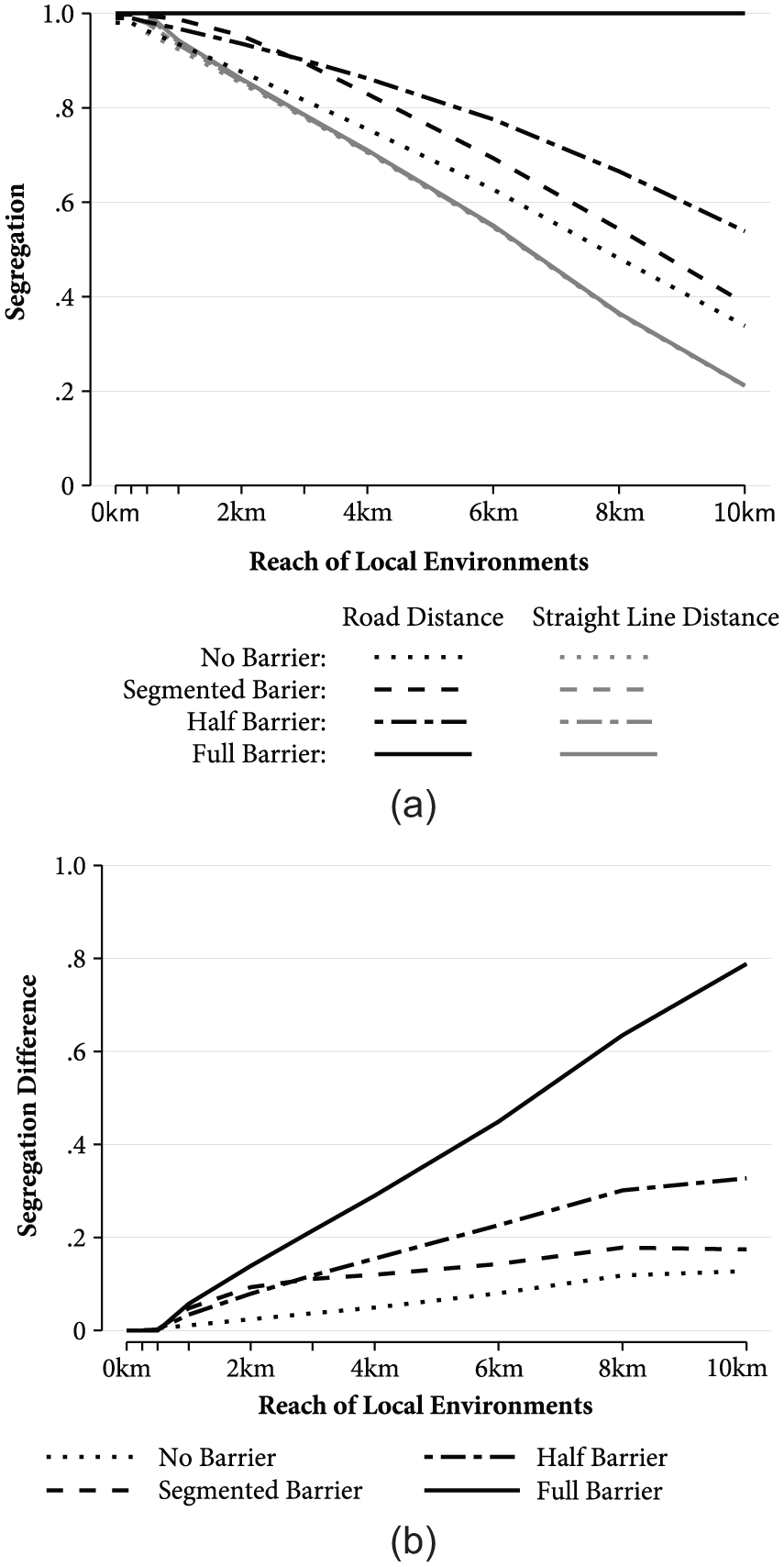
Segregation in a stylized city. (a) Road distance and straight line distance segregation measures by barrier type. (b) Difference between road distance and straight line distance segregation measures by barrier type.

Figure 5.

Maps of road distance segregation in a stylized city by barrier type (reach of local environments = 3 km). (a) No barrier. (b) Full barrier. (c) Partial barrier. (d) Segmented barrier.

Figure 6.

Maps of road distance segregation in a stylized city by barrier type (reach of local environments = 10 km). (a) No barrier. (b) Full barrier. (c) Partial barrier. (d) Segmented barrier.

Figure 5a maps the results for the city with no barriers. Segregation values are highest at the north and south ends of the city and lowest along the midline of the city where the two segregated clusters meet. The city is 12.5 by 12.5 km in size. At a reach of 3 km, only locations relatively near the midline—where black and white residents live in close proximity—experience any change in the composition of their local environments.

With no barriers present, the level of segregation is similar for small local environments using either distance measure, as seen by comparing the dotted black line (road distance) and gray line (straight line distance) in Figure 4a. However, the straight line distance segregation measure shows less segregation, particularly for larger reaches of local environments. The distance between each pair of locations along the road network is longer than the length of a straight line connecting the locations. Given the same reach, local environments are larger when constructed with straight line distance than road distance. They encompass a larger area of the city and include more of the city’s population, which makes their composition more representative of the city’s overall population.

The differences between the two sets of results is due to street design. If the city’s simple street grid was amended to include streets running diagonally through each block, local environments constructed with either distance measure would include the same set of locations, and segregation results would be identical. For example, in cities with avenues that periodically cross diagonally through a grid of streets, as in parts of Washington, D.C., the straight line distance and road distance between two locations is more similar than in cities with a rectangular street grid, as in Midtown Manhattan. The presence of dead-end streets and culs-de-sac has the opposite effect on connectivity: They prevent through movement and increase the difference between the straight line distance and road distance between locations.

Now that I have established the differences in the straight line distance and road distance segregation measures that are attributable to the stylized city’s street design, I separately introduce each of the three barriers into the city and again measure segregation and compare results.

The first barrier fully disconnects the city’s two large clusters and divides the north and south sides of the city (see Figure 5b). As a consequence, local environments constructed with road distance do not include areas on the opposite side of the barrier. Segregation remains at its maximum value even as the reach of local environments increases. Figure 4b shows the difference between the straight line distance and road distance segregation measures for each of the barrier types. Road distance is sensitive to the disconnection imposed by the barrier, but straight line distance is not. Local environments constructed with straight line distance are unchanged by the presence of a barrier. There is maximum segregation in the immediate area of each location, but segregation steadily decreases as the reach of local environments increases.

The full barrier in Figure 5b is an extreme case that is rarely observed at the city level. Figures 5c and 5d show the effect of more realistic partial barriers. The barrier in Figure 5c spans half the city. This creates excess distance between locations on either side of the barrier, but no locations are fully disconnected from the rest of the city. Similarly, in Figure 5d, there is a segmented barrier that creates excess distance but maintains connectivity, similar to a river with bridges every few kilometers. The straight line distance segregation measures show the same results, regardless of whether one of the barriers is present. The effect of the barriers is evident only when using road distance segregation measures.

The presence of a segmented barrier results in higher segregation compared to a city with no barrier. Segregation decreases slowly as local environments increase to a reach of 3 km and then shows a steeper rate of decline beyond that distance. (See again Figure 4a.) The difference narrows when the reach is 10 km and nearly converges with the segregation level for a city with no barrier.

With a barrier that spans half the city’s width, segregation decreases as the reach of local environments increases. The rate of change is steady, but it is more gradual than when no barrier is present. As the reach of local environments increases, the difference in segregation between the city with no barrier and a barrier that spans half the city also increases. (See again Figure 4a.) This is opposite to the trend observed for the city with a segmented barrier where the difference narrowed. This difference occurs because the barriers constrain connectivity in different ways.

Both barriers create excess distance between locations, but the total length of the segmented barrier in Figure 5d is greater than the barrier that spans half the city in Figure 5c. In addition, the segmented barrier is more permeable, allowing connectivity between the two halves of the city at regular intervals. Although the segmented barrier facilitates higher segregation when the reach of local environments is less than 3 km, it is less impactful at greater distances. However, the barrier that spans half the city continues to constrain the local environments of much of the city’s population, even when the reach is 10 km. The difference in the impact of each barrier is evident in Figure 6, which maps the segregation by barrier type for local environments with a reach of 10 km.

4.1.2. “The Other Side of the Tracks” in Pittsburgh

To further demonstrate the application of the SPC method, I examine how connectivity and physical barriers are associated with residential segregation levels in a U.S. city. I measure racial segregation between whites, blacks, Hispanics, and Asians using data from the 2010 decennial census.¹⁵ I measure segregation for local environments with a reach of .5 km, 1 km, 2 km, 3 km, and 4 km. The smallest reach of .5 km approximates the area of a neighborhood in Pittsburgh, and the largest reach of 4 km would include a large portion of the city. I compare the road distance and straight line distance segregation measures for each reach to examine how connectivity and physical barriers influence the segregation levels.

The population of Pittsburgh is 65 percent white, 26 percent black, 4 percent Asian, and 2 percent Hispanic. However, local environments within the city tend to have a different composition than the city. Figure 7 presents the results for the road distance and straight line distance segregation measures. The city-level segregation for local environments with a reach of .5 km is .33 for the straight line distance segregation measure and .37 for the road distance segregation measure. Both segregation measures steadily decrease as the reach of local environments increases, but the level of segregation is consistently higher for the road distance segregation measure.

Figure 7.

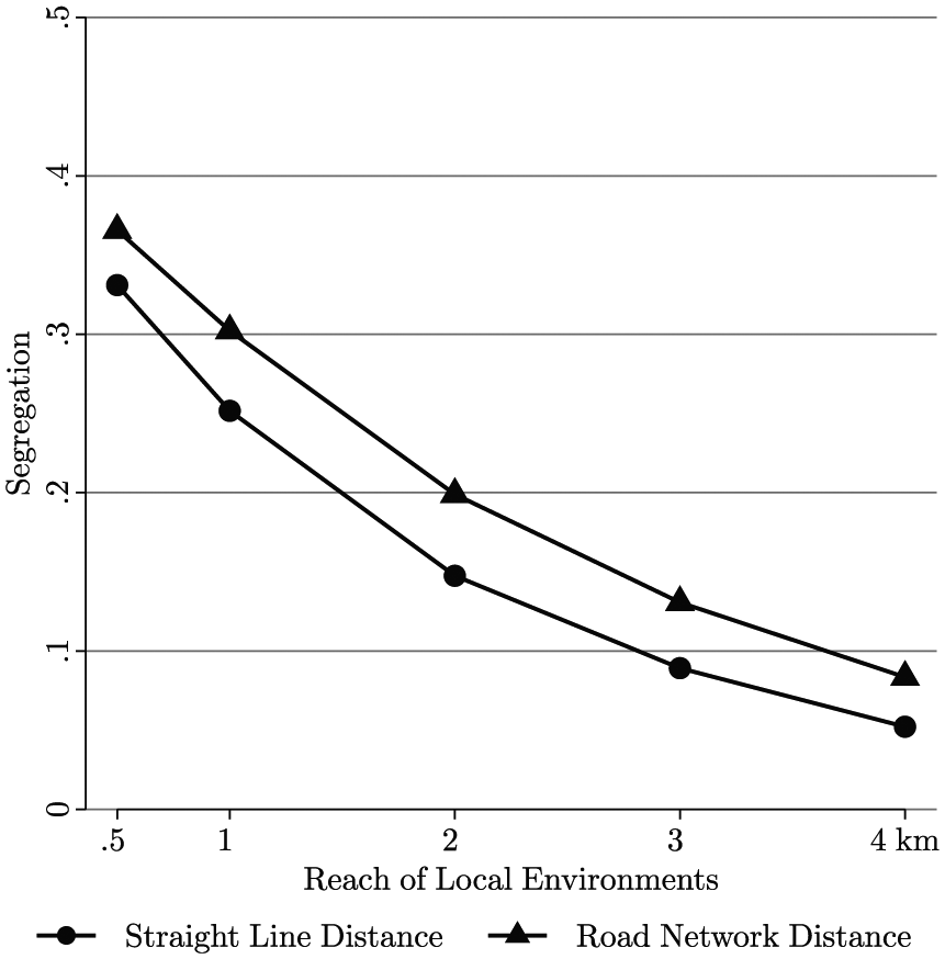
White-black-Hispanic-Asian segregation in Pittsburgh in 2010: a comparison of road distance and straight line distance segregation measures.

The magnitude of the difference between the straight line distance and road distance segregation measures indicates the extent to which physical barriers and disconnectivty influence segregation levels. However, the city-level segregation results for each reach are the population-weighted average of segregation in the local environments of each node, including areas where there are no physical barriers. In such areas, the local environments constructed with road distance and straight line distance will have a similar composition, and there will be no difference between the two segregation measures. Therefore, even small positive differences in the city-level results are meaningful and suggest that physical barriers facilitate greater separation between ethnoracial groups and higher levels of segregation.

The difference between the road distance and straight line distance segregation measures varies considerably across locations in the city. Figure 8 is a map of the differences in local environments with a reach of .5 km. The differences are grouped into quartiles, and the color of each node indicates the magnitude of the difference, with darker colors indicating a greater difference between the measures. There are areas where a cluster of locations all have larger differences between the measures, which indicates that road connectivity or physical barriers in these areas is facilitating higher levels of segregation. A closer inspection of one of these areas illustrates how such differences can arise.

Figure 8.

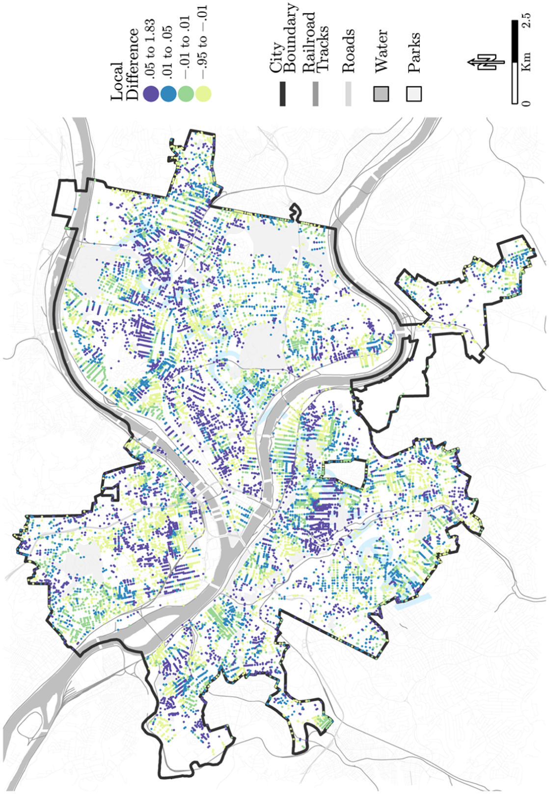
White-black-Hispanic-Asian segregation in Pittsburgh in 2010: quartiles of the difference between road distance and straight line distance segregation measures (reach of local environments = .5 km).

Figure 9 is a map of the local differences between the road distance and straight line distance segregation measures in the Beltzhoover neighborhood of Pittsburgh and other nearby areas.¹⁶ Beltzhoover is located south of downtown Pittsburgh in the Hilltop area of the city. It is bounded on the west and north by railroad tracks and the south by McKinley Park. These features of the built environment reduce the connectivity and increase the distance between Beltzhoover and the neighborhoods of Mount Washington to the west and north and Bon Air to the south. The road network distance between locations in Beltzhoover and these nearby neighborhoods is longer than a straight line connecting the locations. Due to this difference, the local environments of residents in these neighborhoods will differ depending on whether their reach is measured with straight line distance or road distance.

Figure 9.

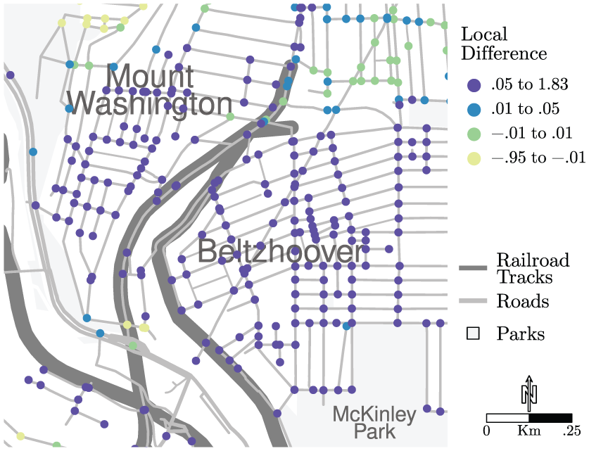
White-black-Hispanic-Asian segregation in an area of Pittsburgh in 2010: quartiles of the difference between road distance and straight line distance segregation measures (reach of local environments = .5 km).

For smaller reaches, such as .5 km, the local environments of locations near the railroad tracks will include areas on opposite sides of the tracks if they are constructed with straight line distance but not if they are constructed with road distance. Figure 2, used as an example in Section 4.1, illustrates this difference. A reach of .5 km is not a sufficient distance to connect the focal location in Beltzhoover to locations on the other side of the tracks in Mount Washington along the road network.

The neighborhoods of Beltzhoover and Mount Washington are physically divided by the railroad tracks, and they also differ in their racial composition. Figure 10 shows a map of the white-black-Hispanic composition in this area of Pittsburgh. The box labeled “City Composition” indicates the color that a node will be if it matches the white-black-Hispanic composition of the city. Most residents on the Beltzhoover side of the tracks are black, and most residents on the Mount Washington side are white. The city of Pittsburgh is 65 percent white and 26 percent black, which is different than the predominantly black composition of Beltzhoover.

Figure 10.

White, black, and Hispanic population in an area of Pittsburgh in 2010.

Because the racial composition of Beltzhoover is surprising given the overall composition of the city’s population, we should expect segregation to be high in the local environments of nodes in Beltzhoover, particularly for smaller reaches measured with road distance. Figure 11 maps the local segregation values for local environments with a .5 km reach, with darker colors indicating higher segregation values. The results for the straight line distance segregation measure are shown in Figure 11a, and the results for the road distance segregation measure are in Figure 11b.

Figure 11.

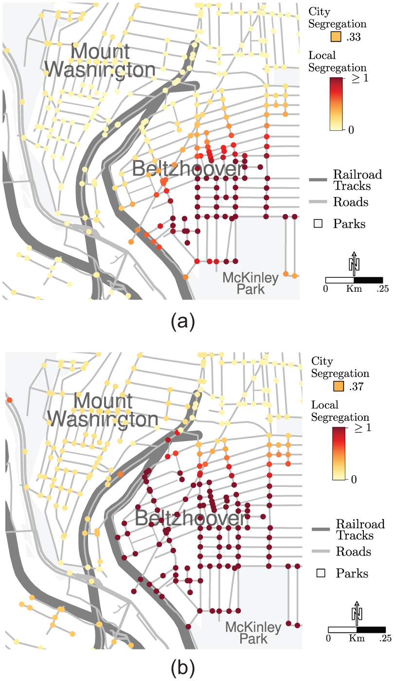
White-black-Hispanic-Asian segregation in an area of Pittsburgh in 2010: straight line distance and road distance segregation measures (reach of local environments = .5 km). (a) Straight line distance segregation measure. (b) Road distance segregation measure.

Comparing the two maps in Figure 11 reveals the extent to which the built environment, including road connectivity and physical barriers, impacts the segregation of these local environments. The segregation values for locations near the railroad tracks in Beltzhoover are higher when their local environments are constructed with road distance rather than straight line distance. The local environments constructed with straight line distance are able to extend into the Mount Washington neighborhood, as was illustrated in Figure 2. In doing so, their racial composition is more representative of the city and therefore less segregated than the local environments constructed with road distance.

Measuring distance along a city’s road network is sensitive to the reduced connectivity and excess distance created by physical barriers. Comparing road distance and straight line distance segregation measures reveals the extent to which disconnectivity and physical barriers facilitate greater separation between groups and increase the local and citywide levels of segregation.

5. Conclusion

The SPC method measures segregation as a function of road network distance to capture how the physical structure of the built environment affects the proximity and connectivity of residential locations. This method lays the foundation for future research examining the spatial structure of segregation patterns, including how it varies across cities and regions, its consequences for residents and communities, and how it has changed over time.

I demonstrated an application of the SPC method with two analyses that compared road distance segregation measures and straight line distance segregation measures to examine how physical barriers and disconnectivity influence residential segregation levels. The first analysis compared how segregation differs in a stylized city when various types of physical barriers spatially separate two groups, and it showed that a barrier’s impact on segregation depends on its spatial configuration and how much it restricts the connectivity between groups. In the second analysis of racial segregation in Pittsburgh, I found that physical barriers and disconnected roads divide urban space in ways that increase the city’s overall level of segregation. However, I also found substantial variation in the impact of barriers across local areas within the city. It is likely that the prevalence of barriers and their impact on segregation levels varies both within cities and across cities as well. By uncovering an additional source of variation in the level of segregation experienced by residents, the SPC method has important implications for understanding the causes and consequences of racial segregation.

There is a long history of physical barriers, such as highways and railroad tracks, being used to reinforce or exacerbate segregation in U.S. cities by facilitating greater separation between groups in nearby areas (e.g., Jackson 1985; Mohl 2002; Schindler 2015; Sugrue 2005). The SPC method contributes to the scholarship on residential segregation by capturing the effect of this additional mechanism of segregation—the connectivity, or physical barriers, between locations—on the level and spatial pattern of segregation.

The SPC method can be used to investigate the role of the built environment in segregation processes by pairing the method with historical data. Comparing road distance segregation measures and straight line distance segregation measures over time can reveal how changes to the built environment, such as the construction or removal of an urban highway, contribute to entrenched patterns of segregation or a shift toward residential integration. In this way, the method can be used to examine how the built environment has contributed to the persistence of residential segregation over the course of the twentieth century.

The SPC method can also be paired with ethnographic fieldwork to provide a more comprehensive account of how the built environment shapes individuals’ interactions and residential contexts. For example, Korver-Glenn’s (2014) ethnographic study of the Northside neighborhood in Houston, Texas, found that the construction of a new transit rail line contributed to high levels of physical division and conflict within the community. The study suggests that road connectivity and physical barriers affect the community aspects of neighborhoods—how residents relate to one another. A mixed-methods approach that integrates the SPC method and ethnographic observation can investigate both the spatial structure and local experience of segregation and offer new insight about the role of the built environment in alleviating or perpetuating residential inequality.

Although the SPC approach improves on the current methods for measuring spatial segregation, there are two issues that present challenges to its implementation. First, the method requires detailed spatial data, which are only available in digital format for the most recent census years. A historical analysis of segregation patterns using the SPC method would require the collection and digitization of street maps and block boundaries from previous census years. Second, the spatially detailed measurement and analysis required by the SPC method is computationally intensive. The processing, memory, and storage demands of the method may not be feasible for many personal computers. For example, the road network data for the city of Pittsburgh includes approximately 19,000 nodes. Thus, calculating the road network distance requires finding the shortest path between 186 million pairs of nodes and storing the result in a large distance matrix. An additional matrix containing proximity weights is computed for every reach of the local environments. The 12 matrices used in the demonstration analysis required about 35 gigabytes of data storage, and the measurement and analysis was conducted in a high-performance computing environment. Given the rapid rate of technological advancements, including the availability of high-performance computing facilities and personal computers with multiple core processors and large memory and storage capacities, the computational demands of the method will become increasingly easy to meet.

Despite these limitations, the SPC method can be extended to incorporate additional aspects of proximity and connectivity into the measurement of racial segregation or applied to measure the spatial segregation or inequality of other population and environmental characteristics, such as income, crime, or environmental hazards.

One way to extend the SPC method is to incorporate different sources of connectivity. For example, to study if the connectivity provided by public transportation facilitates greater separation between groups and higher levels of segregation, the SPC method can use a network of transit routes and stations instead of a road network (or the connectivity provided by both transit and roads can be integrated into a single network). Or, the road network could be constructed as a directed graph if, for example, we wanted to represent the differences in connectivity provided by one-way versus two-way streets. Furthermore, the method can incorporate additional information about the quality of the connectivity provided by roads and other pathways. For example, a bridge or underpass that is desolate or poorly lit may perpetuate separation between nearby areas rather than bringing them together. A measure of the quality of connective roads could further enhance the SPC approach, and new methods for systematic social observation using Google Street View could provide a starting point for developing such a measure (Hwang and Sampson 2014).

The SPC method can also accommodate alternative theories of proximity. If we were interested in measuring segregation as a function of population count (i.e., to control for differences in population density across cities or neighborhoods), the reach of the local environments could be based on the count of nearest neighbors rather than the distance between nodes. Or, if we were concerned with spatial mobility rather than spatial structure, the travel time between nodes could be used to define the reach of local environments instead of road network distance. Such an extension of the SPC method may be relevant to research that uses an activity space perspective to study segregation across the many social and geographic spaces where individuals travel and spend time on a day-to-day basis (Jones and Pebley 2014; Schnell and Yoav 2001; Wong and Shaw 2011; Zenk et al. 2011) or related research that uses geo-ethnography to study the activity patterns that link people to places (Matthews 2011).

I designed the SPC method to create a more accurate and comprehensive portrait of the physical environment of individuals’ residential spaces and develop a deeper understanding of how the built environment influences the patterns, processes, and consequences of segregation. My approach highlights the unique role of the built environment in spatially structuring segregation patterns and enables further consideration of its role in the persistence of segregation.

Supplemental Material

SM796871_Appendices – Supplemental material for The Spatial Proximity and Connectivity Method for Measuring and Analyzing Residential Segregation

Supplemental material, SM796871_Appendices for The Spatial Proximity and Connectivity Method for Measuring and Analyzing Residential Segregation by Elizabeth Roberto in Sociological Methodology

Footnotes

Acknowledgements

I wish to thank Julia Adams, Richard Breen, Paul DiMaggio, Jacob Faber, Jackelyn Hwang, Scott Page, and Andrew Papachristos, as well as the attendees of professional meetings and workshops, for their valuable feedback on previous drafts of this research.

Funding

The author disclosed receipt of the following financial support for the research, authorship, and/or publication of this article: This research was supported by the James S. McDonnell Foundation Postdoctoral Fellowship Award in Studying Complex Systems and the Princeton Institute for Computational Science and Engineering (PICSciE) and the Office of Information Technology’s High Performance Computing Center at Princeton University.

ORCID iD

Elizabeth Roberto

Notes

Author Biography

Elizabeth Roberto is an assistant professor in the Department of Sociology at Rice University. She has broad research interests in social and spatial inequality, a substantive focus on residential segregation, and methodological expertise in computational social science and quantitative methods.

References

Ananat

Elizabeth Oltmans

. 2011. “The Wrong Side(s) of the Tracks: The Causal Effects of Racial Segregation on Urban Poverty and Inequality.” American Economic Journal: Applied Economics 3(2):34–66.

Anderson

Elijah

. 1990. Streetwise: Race, Class, and Change in an Urban Community. Chicago: University of Chicago Press.

Atkinson

Rowland

Flint

John

. 2004. “Fortress UK? Gated Communities, the Spatial Revolt of the Elites and Time-space Trajectories of Segregation.” Housing Studies 19(6):875–92.

Bader

Michael D. M.

Krysan

Maria

. 2015. “Community Attraction and Avoidance in Chicago: What’s Race Got to Do with It?” Annals of the American Academy of Political and Social Science 660(1):261–81.

Besbris

Max

Faber

Jacob William

Rich

Peter

Sharkey

Patrick

. 2015. “Effect of Neighborhood Stigma on Economic Transactions.” Proceedings of the National Academy of Sciences 112(16):4994–98.

Bischoff

Kendra

. 2008. “School District Fragmentation and Racial Residential Segregation: How Do Boundaries Matter?” Urban Affairs Review 44(2):182–217.

Bivand

Roger S.

Keitt

Tim

Rowlingson

Barry

. 2017. “rgdal: Bindings for the Geospatial Data Abstraction Library.” R package version 1.2-16. Retrieved July 30, 2018 (https://CRAN.R-project.org/package=rgdal).

Bivand

Roger S.

Rundel

Colin

. 2017. “rgeos: Interface to Geometry Engine—Open Source (GEOS).” R package version 0.3-26. Retrieved July 30, 2018 (https://CRAN.R-project.org/package=rgeos).

Blakely

Edward J.

Snyder

Mary Gail

. 1997. Fortress America. Washington, DC: Brookings Institution Press.

10.

Brown

Lawrence A.

Chung

Su-Yeul

. 2006. “Spatial Segregation, Segregation Indices and the Geographical Perspective.” Population, Space and Place 12(2):125–43.

11.

Bruch

Elizabeth E.

2014. “How Population Structure Shapes Neighborhood Segregation.” The American Journal of Sociology 119(5):1221–78.

12.

Charles

Camille Zubrinsky

. 2003. “The Dynamics of Racial Residential Segregation.” Annual Review of Sociology 29:167–207.

13.

Chodrow

Philip S.

2017. “Structure and Information in Spatial Segregation.” Proceedings of the National Academy of Sciences 114(44):11591–96.

14.

City of Pittsburgh. 2017a. “Pittsburgh Neighborhoods.” Retrieved June30, 2017 (http://pghgis-pittsburghpa.opendata.arcgis.com/datasets/87a7e06c5d8440f280ce4b1e4f75cc84_0.zip).

15.

City of Pittsburgh. 2017b. “Pittsburgh Parks.” Retrieved January9, 2018 (http://pghgis-pittsburghpa.opendata.arcgis.com/datasets/e95593cb0a2d4ff194be9694b40614dc_0.zip).

16.

Cover

T. M.

Thomas

Joy A.

2006. Elements of Information Theory. Hoboken, NJ.: Wiley-Interscience.

17.

Crowder

Kyle

South

Scott J.

2008. “Spatial Dynamics of White Flight: The Effects of Local and Extralocal Racial Conditions on Neighborhood Out-migration.” American Sociological Review 73(5):792–812.

18.

Csardi

Gabor

Nepusz

Tamas

. 2006. “The igraph Software Package for Complex Network Research.” InterJournal, Complex Systems 1695:1–9.

19.

Duncan

Otis Dudley

Duncan

Beverly

. 1955. “A Methodological Analysis of Segregation Indexes.” American Sociological Review 20(2):210–17.

20.

Farrell

Chad R.

2008. “Bifurcation, Fragmentation or Integration? The Racial and Geographical Structure of US Metropolitan Segregation, 1990–2000.” Urban Studies 45(3):467–99.

21.

Fischer

Claude S.

Stockmayer

Gretchen

Stiles

Jon

Hout

Michael

. 2004. “Distinguishing the Geographic Levels and Social Dimensions of U.S. Metropolitan Segregation, 1960–2000.” Demography 41(1):37–59.

22.

Fischer

Mary J.

2008. “Shifting Geographies: Examining the Role of Suburbanization in Blacks’ Declining Segregation.” Urban Affairs Review 43(4):475–96.

23.

Folch

David C.

Rey

Sergio J.

2016. “The Centralization Index: A Measure of Local Spatial Segregation.” Papers in Regional Science 95(3):555.

24.

Fotheringham

A. Stewart

Wong

David W. S.

1991. “The Modifiable Areal Unit Problem in Multivariate Statistical-analysis.” Environment and Planning A 23(7):1025–44.

25.

Fowler

Christopher S.

2015. “Segregation as a Multiscalar Phenomenon and Its Implications for Neighborhood-scale Research: The Case of South Seattle 1990–2010.” Urban Geography 37(1):1–25.

26.

Fowler

Christopher S.

Lee

Barrett A.

Matthews

Stephen A.

2016. “The Contributions of Places to Metropolitan Ethnoracial Diversity and Segregation: Decomposing Change across Space and Time.” Demography 53(6):1955–77.

27.

Frankel

David M.

Volij

Oscar

. 2011. “Measuring School Segregation.” Journal of Economic Theory 146(1):1–38.

28.

Grannis

Rick

. 1998. “The Importance of Trivial Streets: Residential Streets and Residential Segregation.” American Journal of Sociology 103(6):1530–64.

29.

Grigoryeva

Angelina

Ruef

Martin

. 2015. “The Historical Demography of Racial Segregation.” American Sociological Review 80(4):814–42.

30.

Hipp

John R.

Boessen

Adam

. 2013. “Egohoods as Waves Washing across the City: A New Measure of ‘Neighborhoods.’”Criminology 51(2):287–327.

31.

Hunter

Albert

. 1974. Symbolic Communities: The Persistence and Change of Chicago’s Local Communities. Chicago: University of Chicago Press.

32.

Hwang

Jackelyn

. 2016. “The Social Construction of a Gentrifying Neighborhood: Reifying and Redefining Identity and Boundaries in Inequality.” Urban Affairs Review 52(1):98–128.

33.

Hwang

Jackelyn

Roberto

Elizabeth

Rugh

Jacob

. Forthcoming. “Residential Segregation in the Twenty-first Century and the Role of Housing Policy.” In Blurred Boundaries, Real Consequences: The Intersection of Public Policy and Race, edited by Grimm

Loke

Baton Rouge, LA: Louisiana State University Press.

34.

Hwang

Jackelyn

Sampson

Robert J.

2014. “Divergent Pathways of Gentrification.” American Sociological Review 79(4):726–51.

35.

Jackson

Kenneth T.

1985. Crabgrass Frontier: The Suburbanization of the United States. New York: Oxford University Press.

36.

Jargowsky

Paul A.

Kim

Jeongda

. 2005. “A Measure of Spatial Segregation: The Generalized Neighborhood Sorting Index.” Working Paper No 05-03, National Poverty Center, University of Michigan, Ann Arbor.

37.

Jones

Malia

Pebley

Anne R.

2014. “Redefining Neighborhoods Using Common Destinations: Social Characteristics of Activity Spaces and Home Census Tracts Compared.” Demography 51(3):727–52.

38.

Kane

Michael J.

Emerson

John W.

Weston

Stephen

. 2013. “Scalable Strategies for Computing with Massive Data.” Journal of Statistical Software 55(14):1–19.

39.

Kim

Hwahwan

Yao

Xiaobai

. 2010. “Pycnophylactic Interpolation Revisited: Integration with the Dasymetric-mapping Method.” International Journal of Remote Sensing 31(21):5657–71.

40.

Kim

Young-An

. 2018. “Examining the Relationship between the Structural Characteristics of Place and Crime by Imputing Census Block Data in Street Segments: Is the Pain Worth the Gain?” Journal of Quantitative Criminology 34(1):67–110.

41.

Korver-Glenn

Elizabeth

. 2014. “Middle-class Mexican Americans, Neighborhood Affect, and Redevelopment in Houston’s Northside Barrio.” City & Community 13(4):381–402.

42.

Kramer

Rory

. 2017. “Defensible Spaces in Philadelphia: Exploring Neighborhood Boundaries through Spatial Analysis.” RSF: The Russell Sage Foundation Journal of the Social Sciences 3(2):81.

43.

Krysan

Maria

Bader

Michael D. M.

2009. “Racial Blind Spots: Black-white-Latino Differences in Community Knowledge.” Social Problems 56(4):677–701.

44.

Kullback

Solomon

. 1987. “Letters to the Editor.” The American Statistician 41:338–41.

45.

Lee

Barrett A.

Reardon

Sean F.

Firebaugh

Glenn

Farrell

Chad R.

Matthews

Stephen A.

O’Sullivan

David

. 2008. “Beyond the Census Tract: Patterns and Determinants of Racial Segregation at Multiple Geographic Scales.” American Sociological Review 73(5):766–91.

46.

Lichter

Daniel T.

Parisi

Domenico

Taquino

Michael C.

2015. “Toward a New Macro-segregation? Decomposing Segregation within and between Metropolitan Cities and Suburbs.” American Sociological Review 80(4):843–73.

47.

Logan

John R.

2013. “The Persistence of Segregation in the 21st Century Metropolis.” City & Community 12(2):160–68.

48.

Logan

John R.

2017. “Racial Segregation in Postbellum Southern cities: The Case of Washington, D.C.” Demographic Research 36:1759–84.

49.

Logan

John R.

Zhang

Weiwei

Hongwei

. 2010. “Applying Spatial Thinking in Social Science Research.” GeoJournal 75(1):15–27.

50.

Low

Setha M.

2001. “The Edge and the Center: Gated Communities and the Discourse of Urban Fear.” American Anthropologist 103(1):45–58.

51.

Massey

Douglas S.

2016. “Residential Segregation Is the Linchpin of Racial Stratification.” City & Community 15(1):4–7.

52.

Massey

Douglas S.

Denton

Nancy A.

1988. “The Dimensions of Residential Segregation.” Social Forces 67(2):281–315.

53.

Massey

Douglas S.

Denton

Nancy A.

1993. American Apartheid: Segregation and the Making of the Underclass. Cambridge, MA: Harvard University Press.

54.

Massey

Douglas S.

Rothwell

Jonathan

Domina

Thurston

. 2009. “The Changing Bases of Segregation in the United States.” The ANNALS of the American Academy of Political and Social Science 626(1):74–90.

55.

Matthews

Stephen A.

2011. “Spatial Polygamy and the Heterogeneity of Place: Studying People and Place via Egocentric Methods.” Pp. 35–55 in Communities, Neighborhoods, and Health Expanding the Boundaries of Place, edited by Burton

L. M.

Kemp

S. P.

Leung

Matthews

S. A.

Takeuchi

D. T.

New York: Springer.

56.

Mohl

Raymond A.

2002. “The Interstates and the Cities: Highways, Housing, and the Freeway Revolt.” Retrieved October 5, 2016 (https://www.prrac.org/pdf/mohl.pdf).

57.

Mora

Ricardo

Ruiz-Castillo

Javier

. 2011. “Entropy-based Segregation Indices.” Pp. 159–94 in Sociological Methodology, vol. 41, edited by Liao

T. F.

Thousand Oaks, CA: Sage Publications.

58.

Morrill

Richard L.

1991. “On the Measure of Geographic Segregation.” Geography Research Forum 11(1):25–36.

59.

Neal

Zachary P.

2012. The Connected City: How Networks Are Shaping the Modern Metropolis. New York: Routledge.

60.

Neuwirth

Erich

. 2014. “RColorBrewer: ColorBrewer Palettes.” R package version 1. 1–2. Retrieved July 30, 2018 (http://cran.r-project.org/web/packages/RColorBrewer/index.html).

61.

Openshaw

1984. “Ecological Fallacies and the Analysis of Areal Census Data.” Environment and Planning A 16(1):17–31.

62.

Openshaw

Stanley

Taylor

Peter

. 1979. “A Million or so Correlation Coefficients: Three Experiments on the Modifiable Area Unit Problem.” Pp. 127–44 in Statistical Applications in the Spatial Sciences, edited by Wrigley

London: Pion.

63.

O’Sullivan

David

Wong

David W. S.

2007. “A Surface-based Approach to Measuring Spatial Segregation.” Geographical Analysis 39(2):147–68.

64.

Páez

Antonio

Scott

Darren M.

2004. “Spatial Statistics for Urban Analysis: A Review of Techniques with Examples.” GeoJournal 61(1):53–67.

65.

Parisi

Domenico

Lichter

Daniel T.

Taquino

Michael C.

2011. “Multi-scale Residential Segregation: Black Exceptionalism and America’s Changing Color Line.” Social Forces 89(3):829–52.

66.

Pebesma

Edzer J.

Bivand

Roger S.

2005. “Classes and Methods for Spatial Data in R.” R News 5(2).

67.

Quillian

Lincoln

. 2012. “Segregation and Poverty Concentration: The Role of Three Segregations.” American Sociological Review 77(3):354–79.

68.

R Core Team. 2014. R: A Language and Environment for Statistical Computing. Vienna, Austria: R Foundation for Statistical Computing.

69.

Reardon

Sean F.

Bischoff

Kendra

. 2011. “Income Inequality and Income Segregation.” American Journal of Sociology 116(4):1092–153.

70.

Reardon

Sean F.

Farrell

Chad R.

Matthews

Stephen A.

O’Sullivan

David

Bischoff

Kendra

Firebaugh

Glenn

. 2009. “Race and Space in the 1990s: Changes in the Geographic Scale of Racial Residential Segregation, 1990–2000.” Social Science Research 38(1):55–70.

71.

Reardon

Sean F.

Firebaugh

Glenn

. 2002. “Measures of Multigroup Segregation.” Pp. 33–67 in Sociological Methodology, vol. 32, edited by Stolzenberg

R. M.

Boston, MA: Blackwell Publishers.

72.

Reardon

Sean F.

Matthews

Stephen A.

O’Sullivan

David

Lee

Barrett A.

Firebaugh

Glenn

Farrell

Chad R.

Bischoff

Kendra

. 2008. “The Geographic Scale of Metropolitan Racial Segregation.” Demography 45(3):489–514.

73.

Reardon

Sean F.

O’Sullivan

David

. 2004. “Measures of Spatial Segregation.” Pp. 121–62 in Sociological Methodology, vol. 34, edited by Stolzenberg

R. M.

Boston, MA: Blackwell Publishers.

74.

Revolution Analytics and Steve Weston. 2014. “foreach: Foreach looping construct for R.” R package version 1.4.4. Retrieved July 30, 2018 (https://CRAN.R-project.org/package=foreach).

75.

Roberto

Elizabeth

. 2016. “The Divergence Index: A Decomposable Measure of Segregation and Inequality.” arXiv.org . Retrieved December5, 2016 (http://arxiv.org/abs/1508.01167v2).

76.

Sampson

Robert J.

Sharkey

Patrick

. 2008. “Neighborhood Selection and the Social Reproduction of Concentrated Racial Inequality.” Demography 45(1):1–29.

77.

Schindler

Sarah

. 2015. “Architectural Exclusion: Discrimination and Segregation through Physical Design of the Built Environment.” The Yale Law Journal 124(6):1934–2024.

78.

Schnell

Yoav

2001. “The Sociospatial Isolation of Agents in Everyday Life Spaces as an Aspect of Segregation.” Annals of the Association of American Geographers 91(4):622–36.

79.

Spielman

Seth E.

Logan

John R.

2013. “Using High-resolution Population Data to Identify Neighborhoods and Establish Their Boundaries.” Annals of the Association of American Geographers 103(1):67–84.

80.

Sugrue

Thomas J.

2005. The Origins of the Urban Crisis: Race and Inequality in Postwar Detroit. Princeton, NJ: Princeton University Press.

81.

Suttles

Gerald D.

1972. The Social Construction of Communities. Chicago, IL: University of Chicago Press.

82.

Taeuber

Karl E.

Taeuber

Alma F.

1965. Negroes in Cities: Residential Segregation and Neighborhood Change. Chicago, IL: Aldine Publishing.

83.

Tobler

Waldo R.

1979. “Smooth Pycnophylactic Interpolation for Geographical Regions.” Journal of the American Statistical Association 74(367):519–30.

84.

U.S. Census Bureau. 2011. “2010 Census Summary File 1—United States.” [machine-readable data files]/ prepared by the U.S. Census Bureau.

85.

U.S. Census Bureau. 2012. “2010 TIGER/Line Shapefiles.” [machine-readable data files]/ prepared by the U.S. Census Bureau.

86.

White

Michael J.

1983. “The Measurement of Spatial Segregation.” American Journal of Sociology 88(5):1008–18.

87.

Wong

David W. S.

Shaw

Shih-Lung

. 2011. “Measuring Segregation: An Activity Space Approach.” Journal of Geographical Systems 13(2):127–45.

88.

X. Ben

Sui

Daniel Z.

2001. “An Initial Exploration of a Lacunarity-based Segregation Measure.” Environment and Planning B: Planning and Design 28(3):433–46.

89.

Hongwei

Logan

John R.

Short

Susan E.

2014. “Integrating Space with Place in Health Research: A Multilevel Spatial Investigation Using Child Mortality in 1880 Newark, New Jersey.” Demography 51(3):811–34.

90.

Zenk

Shannon N.

Schulz

Amy J.

Matthews

Stephen A.

Odoms-Young

Angela

Wilbur

JoEllen

Wegrzyn

Lani

Gibbs

Kevin

Braunschweig

Carol

Stokes

Carmen

. 2011. “Activity Space Environment and Dietary and Physical Activity Behaviors: A Pilot Study.” Health and Place 17(5):1150–61.

Supplementary Material

Please find the following supplemental material available below.

For Open Access articles published under a Creative Commons License, all supplemental material carries the same license as the article it is associated with.

For non-Open Access articles published, all supplemental material carries a non-exclusive license, and permission requests for re-use of supplemental material or any part of supplemental material shall be sent directly to the copyright owner as specified in the copyright notice associated with the article.

0.00 MB

0.13 MB