A New RCM Approach to Survival Analysis: The Conditional-Incidence-Rate Model

Abstract

This article introduces a new causal analytic method for survival analysis that retains the framework of Rubin’s causal model as an alternative to the marginal structural model (MSM). The major limitation of the MSM is a systematic bias in the effects of past treatments when the method is applied to the hazard rate analysis of nonrepeatable events in the presence of unobserved heterogeneity. This systematic bias is demonstrated in the article. The method introduced here assumes a semiparametric conditional-incidence-rate model and provides consistent estimates of the effects of present and past treatments on the conditional cumulative-incidence rate in the analysis of nonrepeatable events in the presence of unobserved heterogeneity. Unlike the MSM, which requires a sequential and cumulative use of the inverse-probability-of-treatment weighting many times for data with many time points, the new method uses the inverse-probability-of-treatment weighing only twice sequentially for estimation of the present and past treatment effects at each time of entry into treatment, and not cumulatively across different treatment entry times. Analysis of the conditional-incidence rate can also provide a more efficient parameter estimate for the treatment effect than the hazard rate model in cases where a majority of sample persons experience the event and thereby cease to be members of the risk set of the hazard rate during the period of observation. An application to an analysis of sexual initiation demonstrates that leaving home promotes sexual initiation, especially premarital sexual initiation, because it greatly increases the rate of premarital sexual initiation during the year after leaving home.

Keywords

survival analysis Rubin’s causal model incidence rate unobserved heterogeneity marginal structural model nonrepeatable event

Unobserved Population Heterogeneity, Endogenous Sample Selection Bias, and the Collider-Variable Control Problem in Analysis of Hazard Rates

This article introduces a new semiparametric approach to the causal analysis of event-history data that retains the framework of Rubin’s causal model (RCM). For a semiparametric causal analysis of event-history data, prior work has proposed using a marginal structural model (MSM), which is also an RCM (Barber, Murphy, and Verbitsky 2004; Hernán, Brumback, and Robins 2000; Robins, Hernán, and Brumback 2000). This article shows that although this semiparametric approach is useful in the analysis of panel data, the MSM for hazard rate analysis has a serious limitation. In particular, I show that the MSM for hazard rate cannot provide a consistent estimate for the parameter of interest in the presence of the following three conditions: (1) unobserved heterogeneity in the hazard rate exists, (2) we are interested in estimation of both present and past treatments, and (3) the event is nonrepeatable.¹

As I will describe, bias in use of the MSM under the presence of unobserved heterogeneity, and in the use of any parametric hazard rate model that does not take into account unobserved population heterogeneity, occurs in the effects of “the past treatment.” The “effect of the past treatment” implies here the effect of the treatment variable that is one time unit, in the discrete-time expression, after the time of entry into treatment. Hence, if we assess, for example, the effect of being married among subjects who got married at time s, it becomes biased at time s+1 and later, unless no effect of marital status on event occurrence exists, because bias in the treatment effect arises from the collider-variable control problem (described below). Hence, the problem in estimation of the effect of the past treatment in the hazard rate model exists universally as long as unobserved population heterogeneity exists.

I introduce an alternative approach to survival analysis that provides consistent estimates of the past as well as the present treatment effects even in the presence of unobserved heterogeneity. The method focuses on the effect of the treatment on the conditional cumulative-incidence rate, rather than on the hazard rate. This article thus makes two distinct methodological contributions. First, I clarify a major limitation of the MSM for analysis of the effects of the present and past treatment effects on event occurrence under the presence of population heterogeneity. Second, I introduce a new semiparametric method for the analysis of event-history data that provides consistent parameter estimates for the present and past treatment effects under the presence of unobserved population heterogeneity.

Generally, the presence of an unobserved confounder that affects both the treatment variable and the outcome variable is the major cause of bias in estimation of the parameter for the treatment effect. Different methods have been developed, such as use of person-specific parameters for modeling panel data, as in the difference-in-differences (DID) estimator, and use of an instrumental variable, but one widely used method of making the treatment effect identifiable is the use of propensity scores under the assumption of strong ignorability. The assumption is that the potential outcomes for a dichotomous treatment variable expressed as Y(1) and Y(0) become independent of the treatment assignment Z, controlling for a set of observed covariates V, such that $(Y (1), Y (0)) ⊥ Z | V$ , or equivalently (a) $Y (0) ⊥ Z | V$ and (b) $(Y (1) - Y (0)) ⊥ Z | V$ (Rosenbaum and Rubin 1983, 1984). Condition (a) implies that pretreatment selection bias into the states of the treatment variable is a function of V and can be eliminated when the values of V are fixed. Condition (b) implies that heterogeneity in the treatment effects is independent of assignment to treatment when the values of V are fixed. Estimation of the average treatment effect (ATE) requires both conditions (a) and (b), but estimation of the average treatment effect for the treated (ATT) requires only condition (a).

In this article, I am concerned with estimation of the ATT for present and past treatment effects in the survival analysis of a nonrepeatable event in the presence of time-constant unobserved heterogeneity, which I refer to as unobserved population heterogeneity, with the unobserved variable denoted by U. If this variable is the only unobserved confounder of the treatment effect, then the first condition of ignorability, $Y (0) ⊥ Z | V$ , can be expressed as $U ⊥ Z | V$ . The second condition can be expressed as the absence of any interaction effects of the treatment variable and U on the outcome. I will express the ignorability assumption by using the notation U instead of potential outcomes.

The presence of unobserved population heterogeneity in the survival analysis of a nonrepeatable event is a serious problem, because the unobserved variable always becomes a confounding variable of the covariates of the hazard rate. Even if the unobserved determinant of the hazard rate is initially uncorrelated with covariates, it becomes correlated with them in the analysis of a nonrepeatable event among sample subjects who remain at risk because of the collider-variable control (Elwert and Winship 2014; Morgan and Winship 2007), and the effects of covariates on the hazard rate become biased except for the “present effect” of time-varying covariates. I will demonstrate this problem in a simple illustrative example and with a formal explanation with respect to the effects of a time-varying treatment variable as the key covariate of the hazard rate.

The collider-variable control problem refers to the fact that if two variables V₁ and V₂ that are uncorrelated affect Y, a control for Y generates a correlation between V₁ and V₂. For example, even if gender and ability are uncorrelated in the population, if there is gender inequality in the opportunity to attain a particular high-status occupation and a higher ability threshold is set for women than for men to attain the occupation, the average ability becomes higher for women than for men, among those who attained the occupation and among those who did not, and thus generates a correlation between gender and ability when occupation is held constant.

Throughout this article, Y(t) denotes a dummy variable for the distinction between the occurrence (Y(t) = 1) and the nonoccurrence (Y(t) = 0) of the event at time t, and Y*(t) is a dummy variable for the distinction between whether the event ever occurred (Y*(t) = 1) or never occurred (Y*(t) = 0) by time t by assuming a nonrepeatable event. Similarly, assuming the treatment occurs at most once for each person, Z(t) denotes a dummy variable for the distinction between the occurrence (Z(t) = 1) and the nonoccurrence (Z(t) = 0) of the treatment at time t, and Z*(t) is a dummy variable for the distinction between whether the subject ever received the treatment (Z*(t) = 1) or never received the treatment (Z*(t) = 0) by time t.

I am especially concerned with the collider-variable control problem regarding the fact that even when the treatment variable and the unobserved variable are conditionally independent, or are made conditionally independent, controlling for covariates at time t– 1, the condition is not satisfied among people at risk at time t anymore because of the imposition of $Y (t - 1) = 0$ on the sample who remain at risk at time t. More formally, even if $U ⊥ Z (t - 1) | V (t - 1)$ holds at time t– 1 among people at risk at time t– 1, $U ⊥ Z (t - 1) | V (t - 1), Y (t - 1) = 0$ does not hold among those who remain at risk at time t when both U and Z(t– 1) affect Y(t– 1) because of the collider-variable control of Y(t– 1) = 0 at time t. This generates bias in the effect of Z(t– 1) on the hazard rate, as I will show in the next section.

In the use of parametric hazard rate models, previous work has handled the issue of unobserved population heterogeneity by introducing a time-constant random variable for unobserved population heterogeneity (Flinn and Heckman 1982; Heckman and Singer 1982; Tuma [1978] 1985; Vermunt 1998; Yamaguchi 1986); these revised models have been called frailty models (Blossfeld, Hamerle, and Mayer 1989). The issue addressed in this article, however, is how to handle, without assuming an outcome equation, unobserved population heterogeneity in estimation of the effect of a time-varying treatment variable in survival analysis.

Semiparametric Methods for Hazard Rate Models with a Time-Varying Treatment Variable: A Review and Discussion based on Two Relatively Simple Cases

I now examine two situations to illustrate the limitations of the MSM for the hazard rate analysis of a nonrepeatable event with a time-varying treatment variable. Generally, as Barber et al. (2004) described, on the basis of the work of Hernán et al. (2000), this semiparametric approach to survival analysis requires a sequential application of the inverse-probability-of-treatment (IPT) weighting on the basis of the assumption of sequential ignorability, which is described later, controlling for past treatment histories. My major reservation regarding this approach is that it does not consider the effects of unobserved population heterogeneity under the presence of endogenous sample selection. Because a control for all past treatment histories makes the description of the problem with the method unnecessarily complicated, I discuss the method by focusing on two special cases for a treatment without a repetition: (1) a hypothetical concrete situation in which no covariate control, and thereby no adjustment to attain the independence of the treatment variables from covariates by the MSM, is necessary, and (2) a general situation with covariates where only the effects of Z(t) and Z(t– 1) on hazard rate at time t exist, and no effect of treatments before time t– 1 exists.

Case 1: A Simple Illustrative Analysis of a Hypothetical Model and Data

Suppose we assume a simple situation in which only the effects of Z(t), Z(t– 1), and a dichotomous unobserved variable U, and neither covariate effects nor time effects, on the hazard rate exist, and the assignment to treatment is completely random. For such a situation, the MSM plays no role because no selection bias into treatment states by covariates exists. For simplicity for a simulation analysis, we further assume that the underlying true model of the hazard rate is given as

h (t) = \exp (- 2.0 - 1.5 Z (t) - 1.0 Z (t - 1) + 1.0 U) .

(1)

We also assume that the proportions of people with U = 1 and U = 0 are 50 percent initially, that at each time of 1 and 2, 20 percent of the population enter the treatment state of Z = 1 completely randomly, and that the numbers of event occurrences expected from the model of equation (1) are exactly generated.

Table 1 presents, by assuming the total number of 100,000 people, the number of people at risk, the expected number of people who will experience the event, the hazard rate, and the logarithm of hazard at times 1 and 2 for each combination of Z and U values and each combination of Z values when the expected numbers are summed over the two values of U.

Table 1.

Results for the Model of Equation 1

Latent Class	Time	Treatment State	Expected Number of People at Risk	Expected Number of Event Occurrences	Hazard Rate	Logarithm of Hazard Rate
U = 1	1	Z(1) = 0	40,000.0	5,413.4	.1353	−2.00
	1	Z(1) = 1	10,000.0	302.0	.0302	−3.50
	2	Z(1) = 0, Z(2) = 0	27,669.3	3,774.6	.1353	−2.00
		Z(1) = 0, Z(2) = 1	6,917.3	208.9	.0302	−3.50
		Z(1) = 1, Z(2) = 1	9,698.0	482.3	.0498	−3.00
U = 0	1	Z(1) = 0	40,000.0	14,715.2	.3679	−1.00
	1	Z(1) = 1	10.000.0	820.9	.0821	−2.50
	2	Z(1) = 0, Z(2) = 0	20,227.9	7,441.4	.3679	−1.00
		Z(1) = 0, Z(2) = 1	5,056.9	415.1	.0821	−2.50
		Z(1) = 1, Z(2) = 0	9,179.2	1,242.3	.1353	−2.00
Total	1	Z(1) = 0	80,000.0	20,128.6	.2516	−1.38
	1	Z(1) = 1	20,000.0	1,122.8	.0561	−2.88
	2	Z(1) = 0, Z(2) = 0	47,898.1	11,186.0	.2335	−1.45
		Z(1) = 0, Z(2) = 1	11,974.3	624.0	.0521	−2.95
		Z(1) = 1, Z(2) = 0	18,877.2	1,725.1	.0914	−2.39

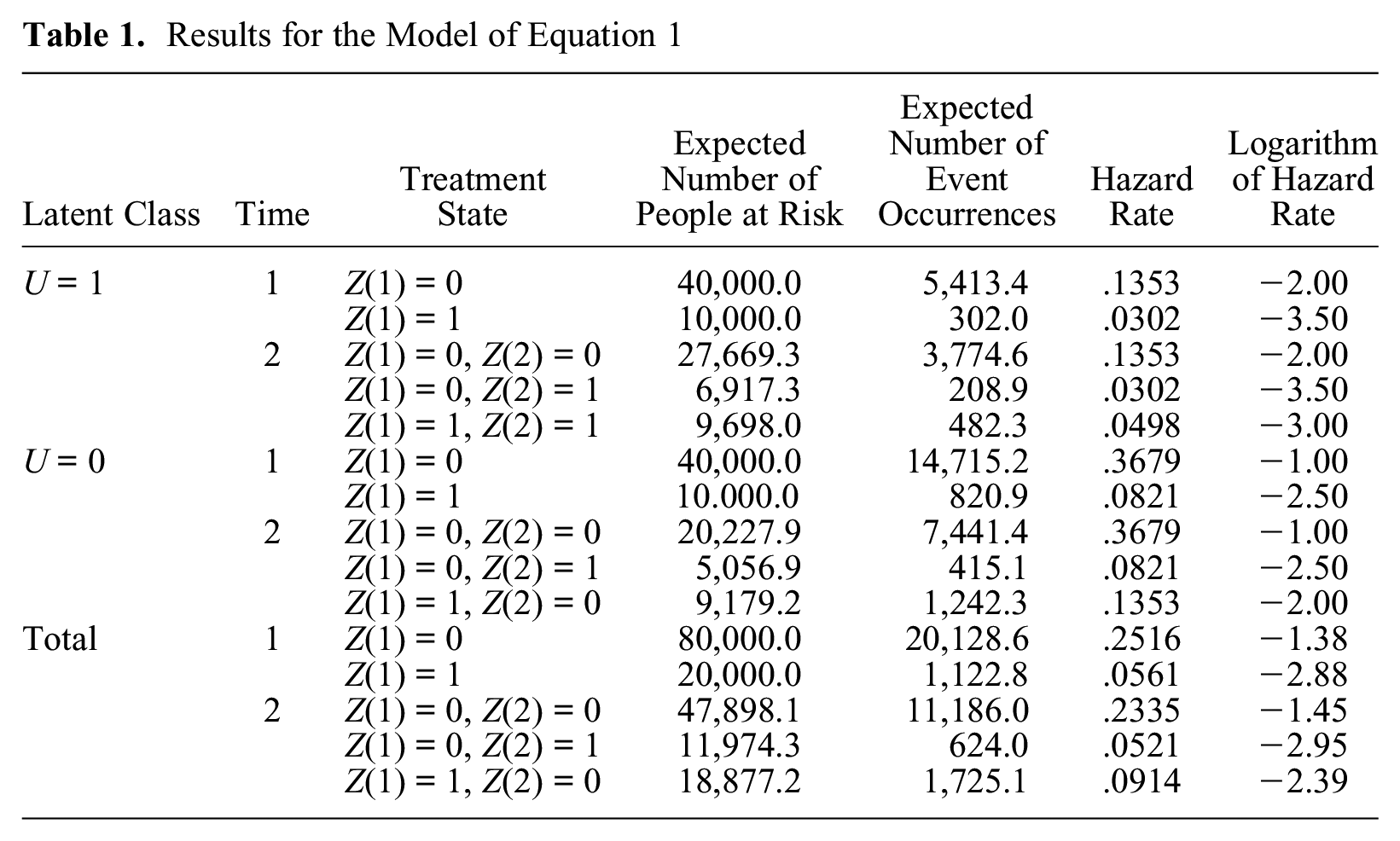
As Table 1 shows, for results aggregated over the two values of U, the effect of the present treatment Z(t) at each time of 1 and 2 becomes equal to the parameter value of –1.5, because it is –2.88 – (–1.38) at time 1 and –2.95 – (–1.45) at time 2, and therefore the estimate of the effect of Z(t) is unbiased at each time even if we ignore the presence of unobserved population heterogeneity. This holds because Z(t) is not correlated with U at either time. However, the effect of Z(t– 1) at time 2 becomes –0.94 (=–2.39 – [–1.45]) and is therefore biased because the parameter value is –1.0. The bias occurs because Z(t– 1) becomes correlated with U among people remaining at risk at time 2. In conclusion, this simple example illustrates that the estimate of Z(t– 1) will be biased when unobserved population heterogeneity exists, and the MSM cannot eliminate this bias because the bias is not caused by observable confounding covariates.

An Explanation for a General Case in Which the Effects of Z(t) and Z(t– 1) on the Hazard Rate Exist

In the case of panel data analysis where the outcome variable Y is observed for the sample during the period of observation unless censoring occurs, the MSM, introduced by Hernán et al. (2000) and by Robins et al. (2000), can provide consistent estimates of the effects of Z(t) and Z(t– 1) under the assumption of sequential ignorability. I first describe the MSM for the analysis of panel data to show the advantage of using the MSM compared with parametric regression models. I then show that if the MSM is used for the hazard rate analysis of a nonrepeatable event, the assumption of sequential ignorability becomes contradictory across time regarding the effect of Z(t– 1) in the presence of unobserved population heterogeneity, and therefore, the MSM cannot identify the parameter for the effect of Z(t– 1) on the hazard rate of a nonrepeatable event.

The Case of Panel Data Analysis

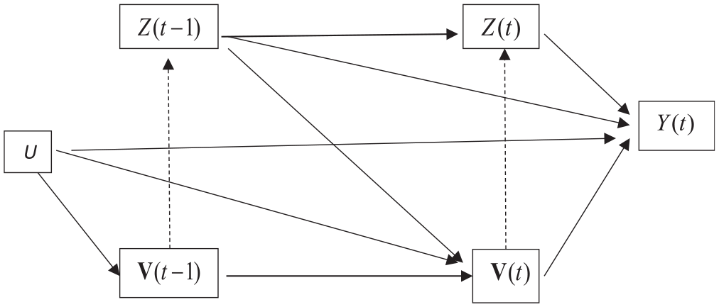
Suppose we assume the causal diagram of Figure 1 for panel data among people who were not treated before time t– 1 or, equivalently, among people with $Z^{*} (t - 2) = 0$ . The characterization of the unobserved variable by a time-constant variable U indicates a simplification made here because the issue I am addressing is the role that unobserved population heterogeneity plays. For comparability with the hazard rate analysis discussed later, I also assume here that treatment occurs at most once, and therefore, assignment to treatment occurs among people who have not yet received treatment. The presence of paths from U to both V(t) and V(t– 1) in the figure indicates that confounding covariates can be endogenous. The absence of direct paths from U to Z(t– 1) and from U to Z(t) indicates that the sequential ignorability assumption described below holds here.

Figure 1.

Causal diagram assumed for estimation of the effects of Z(t – 1) and Z(t) on Y(t) among people with Z*(t – 2) = 0.

Robins et al. (2000) first pointed out that parametric regression models cannot be used to estimate the causal effects of Z(t– 1) and Z(t) on Y(t), and this is the major reason they advocate the MSM. Because covariates V(t) are confounders of the effects of Z(t) on Y(t), they need to be controlled to estimate the causal effects of Z(t) on Y(t). However, covariates V(t) are mediating variables for the effects of Z(t– 1) on Y(t), and therefore, they should not be controlled if the causal effect of Z(t– 1) on Y(t) is to be estimated. These two requirements are contradictory, and therefore parametric regression models do not work for estimation of the causal effects of Z(t– 1) and Z(t) on Y(t).

Robins et al. (2000) pointed out, however, that this problem can be solved by a semiparametric approach that simulates a sequential randomization into the treatment state other than the dependence of Z(t) on Z(t– 1), and this can be done by elimination of the two paths dotted in Figure 1, so that covariates V(t– 1) would no longer be confounders of the effect of Z(t– 1), and covariates V(t) would no longer be confounders of Z(t). Technically, this is attained by making the assumption of sequential ignorability, which is incorporated in Figure 1 such that

U ⊥ Z (t - 1) | V (t - 1), Z^{*} (t - 2) = 0,

(2)

and

U ⊥ Z (t) | V (t), Z^{*} (t - 1) = 0 .

(3)

If the first ignorability assumption of equation (2) holds, we can use propensity score $P (Z (t - 1) | V (t - 1))$ and the derived IPT weights $ω_{t - 1}$ to estimate the ATE of Z(t– 1) on Y(t) as follows:

ω_{t - 1, i} = \frac{P (Z (t - 1) = i)}{P (Z (t - 1) = i | V (t - 1))}, i = 0, 1 .

(4)

Application of these IPT weights to the data eliminates the path from V(t– 1) to Z(t– 1) in Figure 1. Then, under the second ignorability assumption of equation (3), we can eliminate the path from V(t) to Z(t) in Figure 1 while retaining in the data the causal effect of Z(t– 1) on Y(t) obtained by the use of weights $ω_{t - 1}$ , by estimating the propensity score $P_{ω_{t - 1}} (Z (t) | V (t))$ and applying the second IPT weights $ω_{t}$ as follows:

ω_{t, i} = \frac{P_{ω_{t - 1}} (Z (t) = i | Z (t - 1) = 0)}{P_{ω_{t - 1}} (Z (t) = i | V (t), Z (t - 1) = 0)}, i = 0, 1,

(5)

for subjects with $Z (t - 1) = 0$ , where $P_{ω_{t - 1}} (Z (t) | V (t))$ indicates the conditional probability on the basis of data weighted by $ω_{t - 1}$ , and $ω_{t, i} = 1$ for subjects with $Z (t - 1) = 1$ , because no further selection into treatment occurs for those people at time t.

Application of the products of the two weights $ω_{t - 1} ω_{t}$ for the data of time t then generates the causal diagram without two dotted lines in Figure 1, and therefore, the differences

E (ω_{t - 1} ω_{t} Y (t) | Z (t - 1) = 0, Z (t) = 1) - E (ω_{t - 1} ω_{t} Y (t) | Z (t - 1) = 0, Z (t) = 0)

(6)

and

E (ω_{t - 1} ω_{t} Y (t) | Z (t - 1) = 1, Z (t) = 0) - E (ω_{t - 1} ω_{t} Y (t) | Z (t - 1) = 0, Z (t) = 0)

(7)

give the MSM estimate for the effect of Z(t) on Y(t) and the effect of Z(t– 1) on Y(t), respectively.

The Case of Nonrepeatable Events

Now let us consider the case of a causal effect of Z(t) and Z(t– 1) on the hazard rate of a nonrepeatable event, by assuming that only Z(t) and Z(t– 1), and not any treatments further in the past, affect the outcome. To estimate these effects on the hazard rate at time t, we must make a sequential ignorability assumption such that

U ⊥ Z (t - 1) | V (t - 1), Z^{*} (t - 2) = 0, Y^{*} (t - 1) = 0,

(8)

and

U ⊥ Z (t) | V (t), Z^{*} (t - 1) = 0, Y^{*} (t - 1) = 0

(9)

hold at each time t, except for t = 1 for which only assumption (9) is needed. Compared with the sequential ignorability assumption described above for panel data by equations (2) and (3), the condition Y*(t– 1) = 0 is applied for equations (8) and (9), because the hazard rate model at time t is applied only to people who remain at risk without experiencing the event prior to time t for the analysis of a nonrepeatable event. A problem occurs, however, when we assume the same condition to hold at each time t among subjects at risk. In particular, the first ignorability assumption of equation (8) among subjects at risk at t+1 can be expressed as

U ⊥ Z (t) | V (t), Z^{*} (t - 1) = 0, Y^{*} (t) = 0 .

(10)

This condition, however, contradicts the condition of equation (9), because Y(t) is the collider variable of U and Z(t). Hence, even if U and Z(t) are independent by controlling for V(t) at time t, the independence does not hold anymore when a further condition of Y(t) = 0 is imposed at time t+1. Note that Z(t) is the past treatment at time t+ 1, and therefore, the systematic contradiction among the set of ignorability assumptions across time yields bias in the parameter estimate of the past treatment of Z(t– 1) at time t, and it cannot be resolved by making Z(s) independent of V(s) for times of s < t among subjects at risk at each time t by applying IPT weight adjustments of past times repeatedly. It is a problem of contradictions among sequential ignorability assumptions, rather than the problem of realizing independence between the treatment variable and covariates for the past as well as present times in data, as shown by a concrete example in the previous section.

In conclusion, for the analysis of nonrepeatable events, we cannot estimate the causal effect of both Z(t– 1) and Z(t) on Y(t) by application of the MSM by assuming sequential ignorability when unobserved population heterogeneity in the hazard rate exists. Although the problem is shown only for the effect of Z(t– 1) as the simplest example, the effects of any characteristic of past treatment history become biased under the presence of unobserved population heterogeneity in the hazard rate analysis of a nonrepeatable event.

In the next section, I describe a new method that works with the presence of unobserved heterogeneity. This method eliminates the problem of confounding by the unobserved variable by modeling the conditional-incidence rate rather than the hazard rate while retaining a similar sequential ignorability assumption for entry into treatment. The major advantage of this approach is that the constraint Y(t– 1) = 0 does not apply to incidence rate at time t, and it thereby eliminates the problem of endogenous sample selection.

The Conditional-Incidence-Rate Model

The Idea behind the Conditional-Incidence-Rate Model

The method introduced below focuses on the effect of the treatment variable on the conditional-incidence rate of experiencing a nonrepeatable event. This dependent variable has the significant merit of not suffering from the endogenous sample selection problem of hazard rate analysis under unobserved population heterogeneity because the denominator of the incidence rate includes people who have experienced the event.

No parametric incidence-rate model has ever been used in survival analysis because of its inadequacy in handling time-varying covariates. In the hazard rate model, we may assume that the value of a time-varying variable observed at time t, or at time t– 1 if a time lag needs to be made between the predictor and the potential event occurrence, affects the outcome. However, unlike the hazard rate, the incidence rate depends not only on time-dependent covariates observed at time t but also on all the histories of those variables, and those effects may not be log-linearly additive. Hence, it is almost impossible to assume a reasonable parametric model of incidence rates. On the other hand, this issue becomes irrelevant in the semiparametric method because (1) we do not assume any parametric model for the outcome, and therefore we do not need to know the form of covariate effects on the outcome, (2) we only need to control for sample selection into the states of the treatment variable at each time t for which confounding covariates can be assessed by their values at that time, and (3) changes of covariates’ values after entry into treatment should not be controlled for the causal analysis of the treatment effect and are therefore irrelevant.

Because of the absence of sample selection associated with event occurrences, we can expect the MSM can also be applied to analysis of the incidence rate. However, although it is feasible, there is an aspect of clumsiness in the use of the MSM when there are many time points because of its sequential and cumulative application of the IPT weighting, which was described earlier for the analysis of panel data with two time points. In addition, the standard MSM method described by Barber et al. (2004), which preserves the “marginal structure” of both treatment and outcome processes in the IPT-weighted data, does not work under the presence of unobserved heterogeneity because the conditioning on the previous outcomes reintroduces the collider-variable control problem. This is explained further in the section “Estimation of the Past Treatment Effect.”

I introduce an alternative method that greatly simplifies application of the IPT weights. We need to apply only two equations sequentially to estimate propensity scores, separately at each time of entry into treatment, to assess the effects of the present and past treatments under a similar assumption of sequential ignorability. The new method changes the parameters of interest, however, as described below.

I consider a situation in which the time-varying occurrence of treatment is at most once for everybody in the population. The case where the treatment can be repeated makes the estimation of the ATT for time-varying treatment that is the focus of the new method much more complicated technically, so I do not consider it here. Then, if Z(s) = 1 holds for the treatment variable, Z(t) = 0 holds for t > s.

I consider a counterfactual situation separately for each group of people who received treatment at a given time. More concretely, I first consider a counterfactual situation that would have been realized if subjects who got treated at each time had not been treated, that is, I aim at estimating the ATT, for the estimation of the effect of “the present treatment.” I also extend this approach to estimation of the effect of “the past treatment,” as described in the section “Estimation of the Past Treatment Effect.”

An important related issue of analytic strategy is the choice between whether we should assess the treatment effect on the incidence rate per person-period or per person. Incidence rate is time specific, so the rate can be expressed using person-periods of exposure as its denominator, as in the hazard rate. However, incidence rate per person during a fixed time interval [s, t] is the conditional cumulative probability of event occurrence, which is one minus the conditional survival probability, and therefore the analysis of incidence rate per person becomes literally a survival analysis. So, I analyze conditional-incidence rate per person during a fixed time interval, and I manipulate this time interval to examine time variation in the treatment effect. However, I still call the method the conditional-incidence-rate model, rather than the conditional cumulative probability model, because the underlying model is a semiparametric log-rate model of conditional-incidence rate, as described later. In the next sections, I first describe the method for the case with no censored observations and then the method is generalized for the case with censored observations. The handling of censored observations becomes an important methodological issue, as in the hazard rate analysis, when the outcome is concerned with event occurrence during a given time interval.

Parameters and Their Identification for the Case without Censored Observations

Estimation of the “Present” Treatment Effect

The method introduced here distinguishes the following three groups for each time s among subjects who have not yet experienced the event by that time, that is, among those for whom Y*(s– 1) = 0 holds:

a. those for whom Z*(s– 1) = Z(s) = 0,

b. those for whom Z*(s– 1) = 0 and Z(s) = 1, and

c. those for whom Z*(s– 1) = 1.

Selection bias at entry into the treatment state at time s occurs in the difference in the characteristics of people between groups (a) and (b). We call group (a) the control group of entry time s and group (b) the treatment group of entry time s. Note that treatment groups are mutually exclusive across different times of entry into treatment, and the distinction between groups (a) and (b) is a time-constant distinction of the two groups for $t \geq s$ . These two groups of people have the same time interval of observations for a given time interval when censoring does not exist, because we keep people who experience an event occurrence in the analysis of incidence rate. We do not use information about group (c) for estimation of the treatment effect among those who entered treatment at time s.

First, we estimate the effect of Z(s) among people for whom Z*(s– 1) = Y*(s– 1) = 0 on the cumulative probability of the incidence rate during the time interval of [s, s+T_s– 1], where T_s indicates the length of the time interval, on the basis of the following ignorability assumption:

Z (s) ⊥ U | V (s), Z^{*} (s - 1) = 0, Y^{*} (s - 1) = 0,

(11)

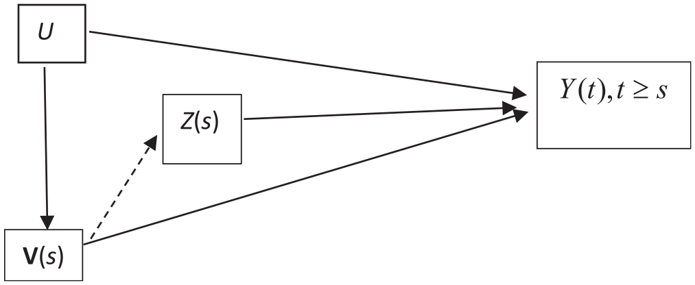
which implies that selection bias into the treatment state at time s among people who had neither a treatment nor an event occurrence prior to time s depends only on the values of covariates V(s). Figure 2 indicates the causal structure of this assumption, where the absence of a direct path from U to Z(s) indicates the ignorability assumption of equation (11).

Figure 2.

A causal structure in which V(s) is the only confounder of the effect of Z(s) on Y(t), where $s \leq t \leq s + T_{s} - 1$ , among people for whom Z*(s– 1) = 0 and Y*(s – 1) = 0 hold.

Figure 2 shows that to estimate the causal effects of Z(s) on Y(t), we only need to eliminate the effects of V(s) on Z(s) indicated by the dashed path in the figure. To estimate the ATT, by conceiving of a counterfactual situation about what would have been the outcomes $Y (t), s \leq t \leq s + T_{s} - 1$ , if people who actually entered the treatment state at time s had not entered the treatment state at that time, we need to apply the following IPT weights to the control group for which Z(s) = 0 holds:

ω (v (s)) = \frac{P (V (s) | Z (s) = 1)}{P (V (s) | Z (s) = 0)} = \frac{P (Z (s) = 0)}{P (Z (s) = 1)} \frac{P (Z (s) = 1 | V (s))}{P (Z (s) = 0 | V (s))} .

(12)

Let $Y_{i}^{s}$ be an individual-specific variable that takes a value of 1 if the event occurs during the time interval of [s, s+T_s– 1], where T_s indicates the time span of observation, and takes a value of 0 otherwise. Note there are no missing observations for $Y_{i}^{s}$ under the condition that no censored observations exist. Hence, $Y_{i}^{s} = \sum_{t = s}^{t = s + T_{s} - 1} Y_{i} (t)$ , and this rate of event occurrence during the time interval of [s, s+T_s– 1], which is equal to the cumulative-incidence rate over the time interval of [s, s+T_s– 1], is given by $E (Y^{s} | Z (s) = 1)$ for the treatment group, and the counterfactual rate that would be realized if subjects with Z(s) = 1 did not enter the treatment state at time s is given by $E (ω (v) Y^{s} | Z (s) = 0)$ on the basis of the weighted data of the control group, and therefore the causal effect of Z(s), denoted by $β_{s}$ , on the outcome is given by

β_{s} = \log (E (Y^{s} | Z (s) = 1)) - \log (E (ω (v) Y^{s} | Z (s) = 0)),

(13)

under the assumption of the log-rate model for the causal effect. Note that the causal estimand here is the logarithm of the rate ratio between the observed group-level cumulative-incidence rate of the treatment group and the corresponding counterfactual rate that would have been realized when people in the treatment group had not received treatment. The rate ratio here is not the same as the ratio of the geometric mean of latent individual-level rates, because the group-level rate is not equal to the geometric mean of the individual-level rates unless rates are homogenous. This disagreement between the average of individual-level parameters and the group-level parameter that we estimate can be eliminated if we assume a linear probability model, and use the difference in the rate, rather than the logarithm of the rate ratio, as the estimator of the treatment effect. However, we use the log-rate model for estimation of the treatment effect because of its significant advantage in handling censored observations, as I will explain in the section “Parameters and Their Identification for the Case with Censored Observations.”

We may estimate the treatment effect averaged over people who entered the treatment state during time [t₁,t₂] by

\bar{β} (t_{1,} t_{2}) = \frac{\sum_{s = t_{1}}^{t_{2}} n_{s} β_{s}}{\sum_{s = t_{1}}^{t_{2}} n_{s}},

(14)

where n_s indicates the number of sample persons who entered the treatment state at time s.²

Estimation of the Past Treatment Effect

Now, let us consider the effect of treatment at one time unit before the present time, as in the case of estimating the effect of Z(t– 1) in the hazard rate model. For simplicity, we refer to this effect as the effect of “the past treatment.” A caveat is necessary in this case: a simple trichotomization of treatment states at treatment entry time s—the state with (1) Z(s) = 1 and Z(s – 1) = 0, that with (2) Z(s) = 0 and Z(s– 1) = 1, and that with (3) Z(s) = 0 and Z(s– 1) = 0 among subjects who were not treated before time s– 1—does not work. This is because we are imposing the condition of Y*(s– 1) = 0 on data to be analyzed for the people of treatment and control groups of entry time s, and because Y*(s – 1) is a collider variable of Z(s– 1) and the unobserved variable U, the distinction between states (2) and (3) is affected by U, and therefore, selection bias into these three states cannot be eliminated by IPT weighting.

We need to consider the effect of the past treatment in a forward-looking manner rather than a backward-looking manner, as described below, by assessing the effect of Z(s) as the effect of the past treatment. In the previous section, we considered the counterfactual situation that people who got treated at time s would have experienced in the time interval of [s, s+T_s– 1] when they had not received treatment at time s. Let us call the outcome under this hypothetical situation the outcome of the counterfactual treatment group. We can regard the difference in the outcome between the observed treatment group and this counterfactual treatment group as the ATT of entry time s for the present treatment.

Suppose now that some subjects of this counterfactual treatment group were randomly assigned to treatment at time s+1, and we refer to those assigned to Z(s+ 1) = 1 as group A and those assigned to Z(s+1) = 0 as group B. Then we can easily see that the difference in the outcome starting from time s+1, that is, the event occurrence during time interval [s+1, s+T_s–1], between group A and group B would reflect the effect of Z(s+1) on the outcome, and the difference in the outcome during the same time interval between the observed treatment group and group B would reflect the effect of Z(s) as the past treatment on the outcome. We can use a strategy of simulating sequential randomization, which is also used in the MSM, to estimate this effect of the past treatment. However, unlike the MSM method described by Barber et al. (2004), our method will not preserve the marginal structure of the outcome process in the creation of a counterfactual situation in the data, because the conditioning on Y(s) reintroduces the collider-variable control problem, as described below.

Thus, the ATT effect of Z(s) as the effect of the past treatment requires us to consider the outcome in the counterfactual situation that people who received the treatment at time s would have experienced during time interval of [s +1, s + T_s–1] when they had received treatment neither at time s nor at time s +1.

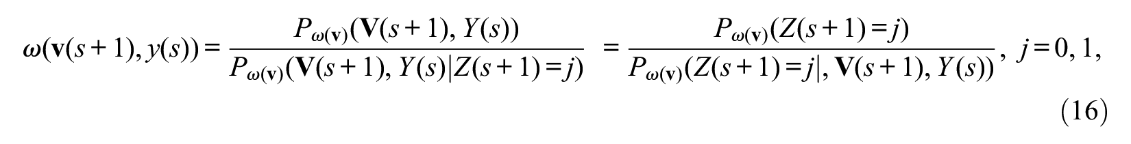
People in the control group do not enter treatment at time s+1 randomly, so we need to eliminate selection bias into the state of Z(s+1). To handle this selection bias, we need to make a similar assumption of sequential ignorability. This implies that in addition to the ignorability assumption of equation (11), we make the following second ignorability assumption regarding entry into treatment at time s+1:

Z (s + 1) ⊥ U | V (t + 1), Y (s), Z^{*} (s) = 0, Y^{*} (s - 1) = 0 .

(15)

A difference in this assumption combined with the assumption of equation (11) from the sequential ignorability assumption of the MSM for hazard rate is that the conditioning factor in equation (15) includes {Y(s), Y*(s– 1) = 0} rather than {Y*(s) = 0} because our analysis includes subjects with Y(s) = 1 as well as Y(s) = 0.

Note that this sequential ignorability assumption does not generate any contradiction here, because unlike the hazard rate analysis, our method does not eliminate samples with Y(s) = 1 at time s+1. However, this fact generates a need to consider the possibility that the outcome at time s, Y(s), may affect Z(s+1). The causal diagram we assume therefore becomes the one presented in Figure 3.

Figure 3.

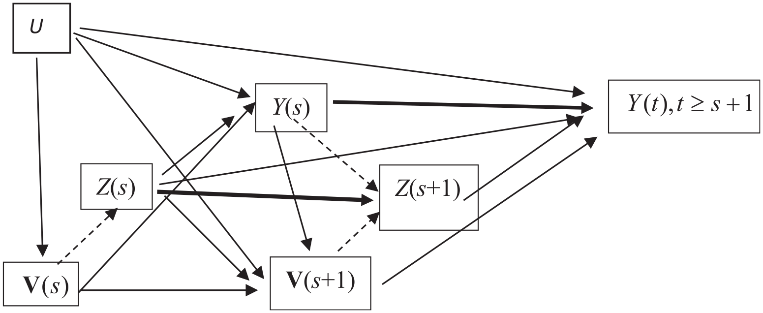
A causal structure for outcomes during the time interval of [s+ 1, s+T_s– 1] after entry into treatment at time s among subjects for whom Z*(s– 1) = 0 and Y*(s– 1) = 0 hold.

In the figure, two thick solid paths, one from Z(s) to Z(s+1) and another from Y(s) to Y(t) for t > s, indicate nonprobabilistic influence such that Z(s+1) = 0 when Z(s) = 1, and Y(t) = 0 for t > s when Y(s) = 1. The figure indicates the following:

The ignorability assumption of equation (11) at time s, indicated by the absence of a direct path from U to Z(s);

The second ignorability assumption of equation (15) at time s+1, indicated by the absence of a direct path from U to Z(s+1);

Selection bias into the state of Z(s+ 1) caused by the effects of V(s+1) and Y(s) on Z(s+1), indicated by dashed paths from V(s+1) and Y(s) to Z(s+1); and

The effect of the unobserved population heterogeneity on entry into the state of Z(s+1), which will be indirect through the effect of U on Y(s), unless a path from Y(s) to Z(s+1) is eliminated.

Note that we cannot retain a path from Y(s) to Z(s+1) and control Y(s) as a covariate of the outcome to block the effect of U on Z(s+1). This is because the control for Y(s) reintroduces the collider-variable control problem and distorts the effect of Z(s) on the outcome. On the other hand, if Y(s) is not held constant while keeping the effect of Y(s) on Z(s+1) in the IPT-weighted data, the effect of Z(s+1) becomes biased not only because U affects Z(s+1) indirectly through its effect on Y(s), but also the effect of Z(s+1) on the outcome reflects a reverse causation.

We must therefore eliminate three paths shown by dashed lines in Figure 3, one from Y(s) to Z(s+1), another from V(s+1) to Z(s+1), and one from V(s) to Z(s), to make the effects of both Z(s) and Z(s+1) on Y(t) for $t \geq s + 1$ be causal effects.

The expression of causality by a diagram is not informative, however, about the question of whether we should use ATT weights or ATE weights, which is a crucial distinction to realize a particular counterfactual situation in data. As described earlier, I estimate the ATT for the effect of Z(s) and therefore use ATT weights to eliminate the path from V(s) to Z(s). To eliminate the two paths from Y(s) to Z(s+1) and V(s+1) to Z(s+1), however, we must use the ATE weights because each group of Z(s+1) = 1 and Z(s+1) = 0 must represent the entire population of the control group to realize the counterfactual situation that would have been realized when people who did not receive a treatment at time s were randomly assigned to treatment at time s+1.

From those considerations, we must estimate the following second IPT weights to eliminate the effects of Y(s) and V(s+1) on Z(s+1) while retaining the joint distribution of Z(s) and V(s) obtained by application of the first IPT weights $ω (v (s))$ among people in the control group:

ω (v (s + 1), y (s)) = \frac{P_{ω (v)} (V (s + 1), Y (s))}{P_{ω (v)} (V (s + 1), Y (s) | Z (s + 1) = j)} = \frac{P_{ω (v)} (Z (s + 1) = j)}{P_{ω (v)} (Z (s + 1) = j |, V (s + 1), Y (s))}, j = 0, 1,

(16)

where $P_{ω (v)}$ indicates the weighted probability measure for data weighted $ω (v (s))$ defined in equation (12). Note that covariates V(s) that affect Z(s+1) directly need to be included as components of V(s+1) so that the weighting by $ω (v (s + 1), y (s))$ preserves the joint distribution of Z(s) and V(s) weighted by $ω (v (s))$ . The IPT weight we need to apply to the data of the control group to estimate the past treatment effect of Z(s) is then given by the product, $ω (v (s)) ω (v (s + 1), y (s))$ , of the weights of equations (12) and (16).

The expected outcome for the cumulative-incidence rate during the time interval [s+1, s+T_s– 1] is defined by excluding the period of time s. Thus, for $Y_{i}^{s + 1} = \sum_{t = s + 1}^{t = s + T_{s} - 1} Y_{i} (t)$ , which takes a value of 1 if the event occurs during the time interval [s+1, s+T_s– 1] and takes a value of 0 otherwise, the observed cumulative-incidence rate for this time interval is given by $E (Y^{s + 1} | Z (s) = 1)$ for the treatment group. The counterfactual expected cumulative-incidence rate that would have been realized if subjects with Z(s) = 1 had not entered the treatment state either at time s or time s+1, is given by $E (ω (v (s)) ω (v (s + 1), y (s)) Y^{s + 1} | Z (s) = 0, Z (s + 1) = 0)$ , on the basis of the weighted data of subjects in the control group with Z(s+1) = 0 weighted by weights $ω (v (s)) ω (v (s + 1), y (s))$ . The effect of the past treatment, $β_{s} (past)$ , is then given by the following formula:

β_{s} (past) = \log (E (Y^{s + 1} | Z (s) = 1)) - \log (E (ω (v (s)) ω (v (s + 1), y (s)) Y^{s + 1}) | Z (s) = 0, Z (s + 1) = 0))

(17)

The ATT over different entry times of treatment can also be given, as in equation (14), as the weighted average of entry time–specific treatment effects, with the number of subjects in the treatment group at each time of entry into treatment as the weight.

Parameters and Their Identification for the Case with Censored Observations

When the observation of Y (t) is censored during the time interval of [s, s+T_s– 1], we have missing outcomes. It follows that if the treatment variable Z(s) affects censoring at time t > s, the effect of Z(s) on the outcome cannot be assessed without making an additional assumption about the ignorability of censoring, because we must eliminate the effect of Z(s) on censoring to assess the treatment effects on the outcome with censored data. However, the method for such an extension leads to a loss of simplicity because the conditioning on the nonoccurrence of censoring requires the IPT weight adjustment to be made at each time when censored observations exist. I do not extend the new method for such cases, because my aim here is to introduce a new method without making any additional ignorability assumption beyond those made in the MSM, and to retain the simplicity of the IPT weighting method. Hence, I assume that the treatment variable does not affect censoring below.

When the treatment variable does not affect censoring, we obtain a very simple result: we can treat censored observations in the same way as the nonoccurrence of the event for the entire period in defining the outcome variable. This holds for the effect of Z(s) as both the effect of the present treatment and the past treatment. This fact is formally proved for the present treatment effect below, and is explained in Appendix A for the past treatment effect, but an explanation of the underlying logic about why we can expect this fact will be useful. The proof results from a combination of three things. First, under the situation in which people are randomly assigned to states of Z(s), and Z(s) does not affect censoring, we can expect that the marginal probability distribution of censoring nonoccurrence will be equal between the treatment group and the control group. Second, as Yamaguchi (2012) showed, data are collapsible over persons in the log-rate model of the treatment effect when the treatment effects are homogenous and the treatment variable is independent, or made independent, of covariates. Third, as stated earlier, we are interested in estimation of the group-level treatment effect of the log-rate model on the cumulative-incidence rate, and the group-level treatment effect is equal to the average of individual-level treatment effects when the latter effects are homogenous. Hence, if we make a working assumption of homogenous treatment effects for the individual-level conditional-incidence rate under the nonoccurrence of censoring, the joint rates of event occurrence and censoring nonoccurrence can be summed across persons without changing the treatment effect. Then, the ratio of those joint rates between the treatment group and the control group will cancel out, under the condition that the covariate distribution is made equal between the two groups, the component of a function of covariates and censoring, and will retain only the component of the treatment effect.

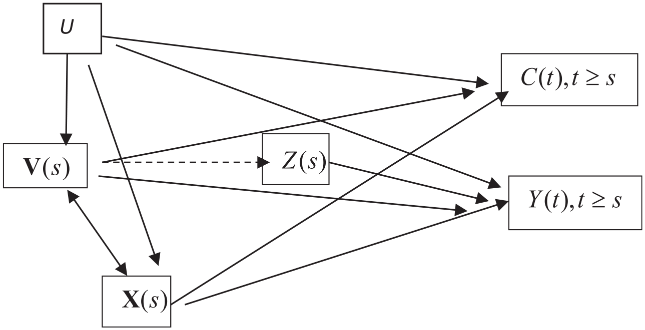
Let me show this fact more formally for the case of the present treatment effect. Figure 4 shows the causal structure including a dummy variable for censoring at time t, C(t) for t > s, where X(s) represents covariates that affect censoring and may affect event occurrence as well, but do not affect the treatment assignment. The absence of a path from Z(s) to C(t) indicates the assumption that the treatment variable does not affect censoring. In Figure 4, no causal relationship between censoring and the outcome is indicated, because the outcome becomes missing at the time of censoring t for people with Y*(t– 1) = 0 and is fixed as Y(t) = 0, for people with Y*(t– 1) = 1.

Figure 4.

A causal structure during the time interval [s, s+T_s– 1] for which the treatment does not affect censoring for the treatment group and the control group of entry time s, for which Z*(s– 1) = 0 and Y*(s– 1) = 0 hold.

We assume the following semiparametric log-rate model of the conditional-incidence rate of event occurrence for person i in the treatment and control groups of entry time s,

\begin{matrix} \log (R_{i} (t | Z^{*} (s - 1) = 0, Y^{*} (s - 1) = 0, C_{si} (t) = 0)) = α_{s, t} + β_{s} Z_{i} (s) + ϕ (V_{i} (s), X_{i} (s)) + U_{i}, \\ for s \leq t \leq s + T_{s} - 1 \end{matrix}

(18)

where the set of $α_{s, t}$ expresses time effects, $β_{s}$ is the “present” treatment effect, $ϕ (V (s), X (s))$ represents the parametrically unspecified effect of observable covariates V and X, and U is the variable for unobserved population heterogeneity that satisfies the ignorability condition of equation (11). Note that this model will not be applied to data but is used to demonstrate the identifiability of the treatment effect $β_{s}$ for this semiparametric model. One may consider the homogeneous effect of Z(s) on the incidence rate to be unrealistic. However, as stated before, this is a working assumption to obtain a consistent estimate for the effect of Z(s) on the cumulative-incidence rate of the treatment group during a given time interval.

This incidence rate is based on two conditions. First, it applies only to the treatment and control groups of entry time s, thereby satisfying Y*(s– 1) = 0 and $Z^{*}$ (s– 1) = 0. Second, it applies under the condition that censoring does not occur, indicated by $C_{si} (t) = 0$ where $C_{si} (t)$ is a dummy random variable that indicates whether censoring for person i occurs by time t ( $C_{si} (t) = 1$ ) or not ( $C_{si} (t) = 0$ ). Below, for simplicity we denote $R (t | Z^{*} (s - 1) = 0, Y^{*} (s - 1) = 0, C (t) = 0)$ as $R_{s} (t | C (t) = 0)$ . Note that covariates after time s are not included in equation (18), because they can be mediating variables for the effect of Z(s) on Y(t), which we should not control. For the same reason, C(t) is assumed to depend on V(s), X(s), and U, and not on Z(s) as indicated in Figure 4, rather than on the values of V and X at time t– 1. The aim of the following analysis is to show that for the log incidence-rate model used here, the observed data become collapsible over persons and times to obtain the estimate of $β_{s}$ .

To show this, we consider the joint rate of event occurrence and censoring nonoccurrence, which can be expressed as $R_{s} (t | C_{s} (t) = 0)) P (C_{s} (t) = 0)$ . Note that $f (v (s), x (s), u | Z (s)) = f (v (s) | Z (s)) f (u, x (s) | v (s), Z (s)) = f (v (s) | Z (s)) f (u, x (s) | v (s))$ , where f(.) denotes the probability density function, holds because Z(s) is assumed to be conditionally independent of (U,X(s)), controlling for V(s), as shown in Figure 4. Then the expected cumulative rate of event occurrence and censoring nonoccurrence, summed over time from s to s+T_s– 1 and over persons for people in the treatment group, is given as

\begin{matrix} \int_{v} [\sum_{t = s}^{s + T_{s} - 1} {\int_{u, x} R_{s} (t | C_{s} (t) = 0, v, x, u, Z (s) = 1) P (C_{s} (t) = 0 | v, x, u) f (u, x | v) dud x}] f (v | Z (s) = 1) d v \\ = \int_{v} [\sum_{t = s}^{s + T_{s} - 1} \exp (α_{s, t} + β_{s}) {\int_{u, x} \exp (ϕ (v, x) + u) P (C_{s} (t) = 0 | v, x, u) f (u, x | v) dud x}] f (v | Z (s) = 1) d v \\ = \exp (β_{s}) \int_{v} [\sum_{t = s}^{s + T_{s} - 1} \exp (α_{s, t}) {\int_{u, x} \exp (ϕ (v, x)) + u) P (C_{s} (t) = 0 | v, x, u) f (u, x | v) dud x}] f (v | Z (s) = 1) d v . \end{matrix}

(19)

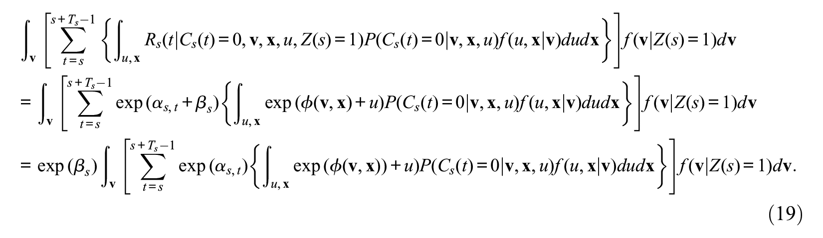
On the other hand, because $ω_{s} (v (s)) f (v | Z (s) = 0) = f (v | Z (s) = 1)$ for the IPT weights defined above, the expected cumulative rate of event occurrence and censoring nonoccurrence for the control group with weights $ω_{s} (v)$ becomes

\begin{matrix} \int_{v} [\sum_{t = s}^{s + T_{s} - 1} {\int_{u, x} R_{s} (t | C_{s} (t) = 0, v, x, u, Z (s) = 0) P (C_{s} (t) = 0 | v, x, u) f (u, x | v) dud x}] ω_{s} (v) f (v | Z (s) = 0) d v \\ = \int_{v} [\sum_{t = s}^{s + T_{s} - 1} \exp (α_{s, t}) {\int_{u, x} \exp (ϕ (v, x) + u) P (C_{s} (t) = 0 | v, x, u) f (u, x | v) dud x}] f (v | Z (s) = 1) d v \\ = \int_{v} [\sum_{t = s}^{s + T_{s} - 1} \exp (α_{s, t}) {\int_{u, x} \exp (ϕ (v, x) + u) P (C_{s} (t) = 0 | v, x, u) f (u, x | v) dud x}] f (v | Z (s) = 1) d v . \end{matrix}

(20)

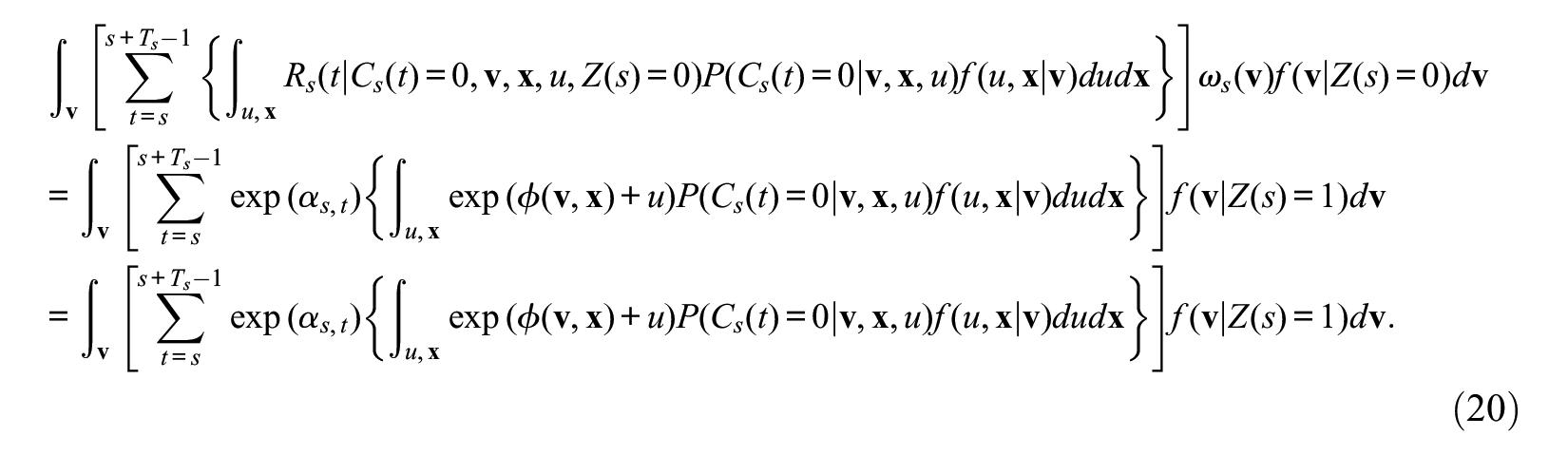
Hence, the ratio of equation (19) to equation (20) is $\exp (β_{s})$ . It follows that the difference between equations (19) and (20) in the logarithm of the cumulative probability of event occurrence and censoring nonoccurrence becomes $β_{s}$ . Hence, censored observations can be treated equally with cases with event nonoccurrence. It follows that under the presence of censored observations, we can define the individual-level outcome variable Y to take a value of 1 if the event occurs during that time interval of [s, s+T_s– 1] and takes a value of 0 when the event does not occur, including censored cases. Then the effect of the present treatment is given by the same formula of $β_{s} = \log (E (Y | Z (s) = 1)) - \log (E (ω (v) Y | Z (s) = 0))$ for the conditional log incidence-rate model for the effect of Z(s).

The identifiability of the effect of Z(s) as the effect of the past treatment from the data of event occurrence during the time interval of [s+1, s+T_s– 1] by treating censored observations the same as the cases of event nonoccurrence is explained in Appendix A.

Notes on Estimation of Parameters and Their Standard Errors

We may use the Huber-White robust estimation (Huber 1964, 1967) for the standard error of treatment effects for each time of entry into treatment because the rate estimate for the control group is weighted by the IPT weight. This can be simply done by using the individual-level outcome variable described earlier, by assuming a working log-rate model of $\exp (α + β_{s} Z)$ with the IPT-weighted data, and by specifying the robust estimation for the standard error. Stata commands for the estimation of the present and past treatment effects of Z(s) for a given time s of entry into treatment are described in Appendix B.

As described in equation (14), the ATT of both the present and past treatment effects over different times of entry into treatment is given as the weighted average of the entry time–specific effects weighted by the sample size of subjects in the treatment group, that is, by $\bar{β} (t_{1,} t_{2}) = \sum_{s = t_{1}}^{t_{2}} n_{s} β_{s} / \sum_{s = t_{1}}^{t_{2}} n_{s}$ . When estimates of the set of { $β_{s}$ } and their standard errors are given by existing software for the log-rate model, we can reasonably assume the estimates are independent across the entry times so that we may estimate the standard error of $\bar{β}$ , as $SE (\bar{β}) = \sqrt{\sum_{s} n_{s}^{2} σ^{2} (\hat{β_{s}})} / \sum_{s} n_{s}$ , although this leads to a slight overestimation of the standard error and leads to a conservative test of significance. It will be an overestimation because estimates of $β_{s}$ will be positively correlated across s because of the commonality of control groups. However, it will be a minor overestimation: if we assume that the outcomes of control groups are fixed, then the estimate $β_{s}$ will be independent because treatment groups across entry times are mutually exclusive. In fact, when outcomes of the control groups for s = 1, which is taken into account in the standard error of $β_{1}$ , are given, there is very little variability of outcomes left for the control groups of time s > 1, because the individual outcomes of people in the control group are all the same across different s values and differ only in the IPT weights. Hence, the standard error obtained by assuming independence of ATT estimates across s is nearly the same as one obtained by assuming that outcomes of control groups are given for entry time s > 1.

Notes on Assessing the Treatment Effects on Event Timing

It is well known that, unlike the hazard rate, the incidence rate cannot reflect differences in the timing of event occurrences. The method described above, however, can assess the treatment effects on the cumulative probability of event occurrence and therefore can solve this issue by analyzing the sum of the conditional-incidence rate from time s to time s+T– 1 for various different values of time interval T. For example, if results show that the treatment effect is significant for T = 1 but absent for T = 5, then this will imply that the treatment affects the timing of event occurrence but not the probability of occurrence over the five periods.

Notes on the Case of a Time-Constant Treatment Variable

Suppose the treatment variable is a characteristic of people at or before entry into the risk for event occurrence, such as the effect of educational attainment at marriage in predicting divorce. Such a time-constant treatment variable also becomes correlated with unobserved heterogeneity, unless the treatment effect is absent, among subjects who remain at risk in the hazard rate model, and therefore the treatment effect becomes biased in the presence of, and no control for, unobserved population heterogeneity. The method for analysis of the conditional-incidence rate introduced in this article can be used to obtain consistent estimates for the effects of such time-constant treatment variables. The method is also greatly simplified in such cases because we only need a one-time ignorability assumption at the time of entry into risk regarding the assignment to treatment. Hence, we need to estimate the IPT weights just once by including all sample subjects who entered the risk at various different times by characterizing them at the time of their entry into risk. The method for the past treatment effect for a time-varying treatment variable becomes irrelevant in this case.

Application

Data and Variables

The application for the new method is based on data from the National Health and Social Life Survey (http://popcenter.uchicago.edu/data/nhsls.shtml) conducted by the University of Chicago in 1992 to analyze the social organization of sexual behavior (Laumann et al. 1994). I use survey data on age at first sexual intercourse, age at first leaving home, and age at first marriage for men and women aged 20 to 59 years. With this dataset, I analyze the rate of two different life events: (1) the occurrence of premarital sexual initiation for which the occurrence of marriage is the competing event and (2) the occurrence of sexual initiation, including through marriage, which I will refer to as “sexual initiation in general,” for the sake of distinction.

Because the survey collects age information only at the time of the event and the competing event, we treat the occurrence of sexual initiation at an age equal to the age at marriage as a censored observation in the analysis of premarital sexual initiation. Hence, among respondents who ever married, premarital sexual initiation implies an occurrence of sexual initiation at a younger age than the age at marriage.

The focal quantity of interest is the causal effect of leaving home as a time-varying treatment variable. To eliminate possible reverse causation, the value of Z(t) in predicting Y(t) is defined with a one-year time lag, so that the subject is treated as having already left home (for which Z(t) = 1) if and only if the subject left home at least one year before time t.

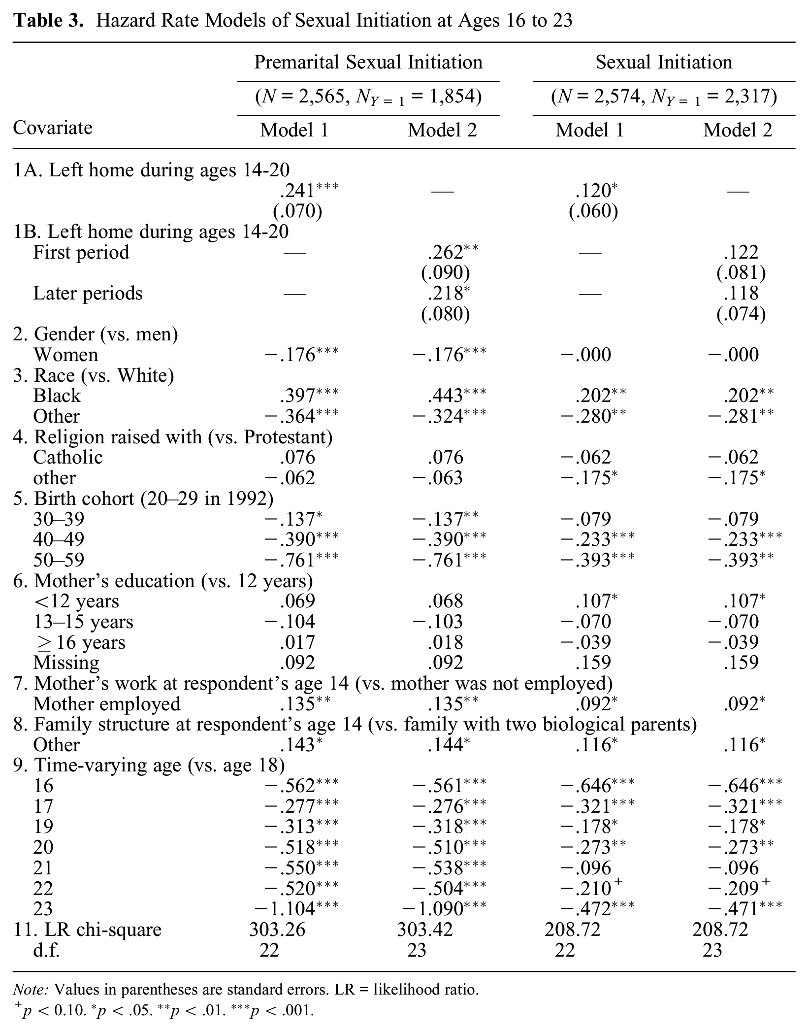
As possible confounding variables, I used seven categorical covariates in addition to the effect of the timing of entry into treatment and time-varying effects of age that are built into the model: (1) gender, (2) race, (3) religion raised with, (4) mother’s education, (5) family characteristics at age 14, (6) whether mother was employed at age 14, and (7) birth cohort. The categories of the seven covariates are shown later in Table 3.

Table 2.

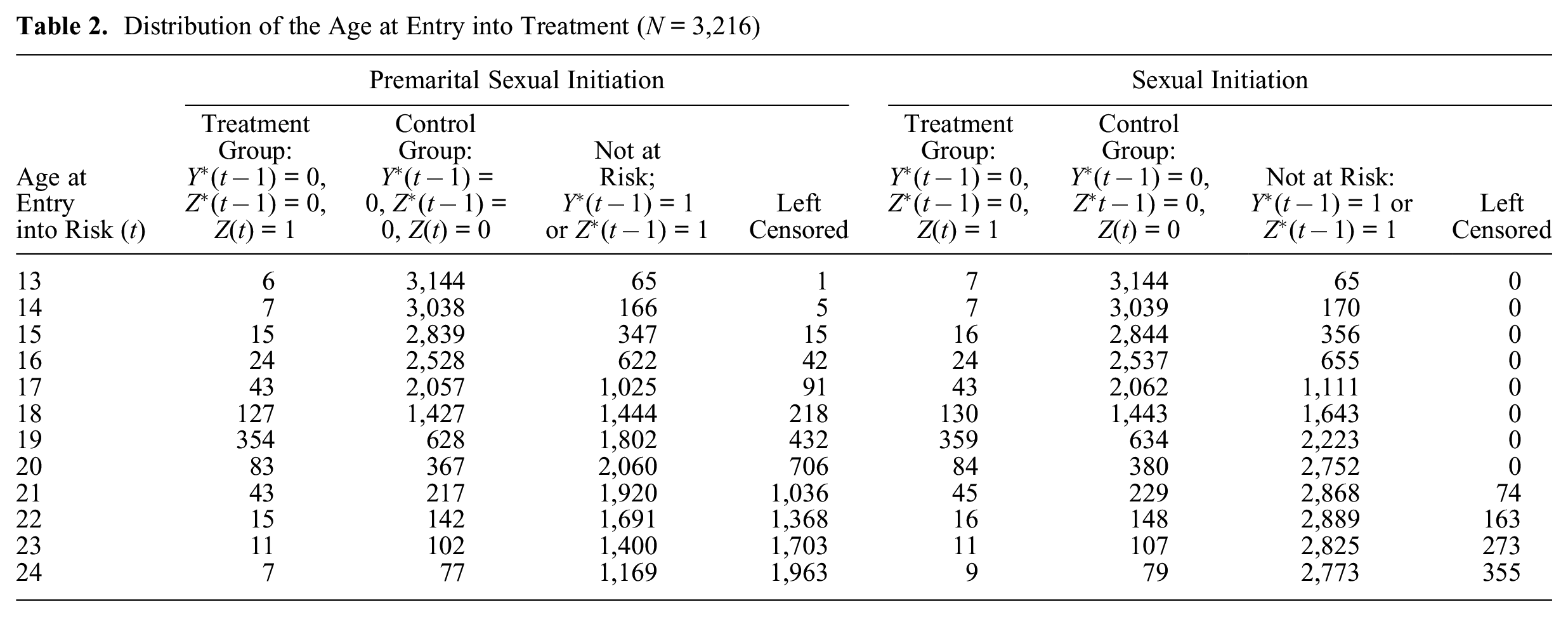
Distribution of the Age at Entry into Treatment (N = 3,216)

	Premarital Sexual Initiation				Sexual Initiation
Age at Entry into Risk (t)	Treatment Group: Y(t– 1) = 0, Z(t– 1) = 0, Z(t) = 1	Control Group: Y(t– 1) = 0, Z(t– 1) = 0, Z(t) = 0	Not at Risk; Y(t– 1) = 1 or Z(t– 1) = 1	Left Censored	Treatment Group: Y(t– 1) = 0, Z(t– 1) = 0, Z(t) = 1	Control Group: Y(t– 1) = 0, Zt– 1) = 0, Z(t) = 0	Not at Risk: Y(t– 1) = 1 or Z(t– 1) = 1	Left Censored
13	6	3,144	65	1	7	3,144	65	0
14	7	3,038	166	5	7	3,039	170	0
15	15	2,839	347	15	16	2,844	356	0
16	24	2,528	622	42	24	2,537	655	0
17	43	2,057	1,025	91	43	2,062	1,111	0
18	127	1,427	1,444	218	130	1,443	1,643	0
19	354	628	1,802	432	359	634	2,223	0
20	83	367	2,060	706	84	380	2,752	0
21	43	217	1,920	1,036	45	229	2,868	74
22	15	142	1,691	1,368	16	148	2,889	163
23	11	102	1,400	1,703	11	107	2,825	273
24	7	77	1,169	1,963	9	79	2,773	355

Table 3.

Hazard Rate Models of Sexual Initiation at Ages 16 to 23

Covariate	Premarital Sexual Initiation		Sexual Initiation
	(N = 2,565, N_Y_{= 1} = 1,854)		(N = 2,574, N_Y_{= 1} = 2,317)
	Model 1	Model 2	Model 1	Model 2
1A. Left home during ages 14-20
	.241*** (.070)	—	.120* (.060)	—
1B. Left home during ages 14-20
First period	—	.262** (.090)	—	.122 (.081)
Later periods	—	.218* (.080)	—	.118 (.074)
2. Gender (vs. men)
Women	−.176***	−.176***	−.000	−.000
3. Race (vs. White)
Black	.397***	.443***	.202**	.202**
Other	−.364***	−.324***	−.280**	−.281**
4. Religion raised with (vs. Protestant)
Catholic	.076	.076	−.062	−.062
other	−.062	−.063	−.175*	−.175*
5. Birth cohort (20–29 in 1992)
30–39	−.137*	−.137**	−.079	−.079
40–49	−.390***	−.390***	−.233***	−.233***
50–59	−.761***	−.761***	−.393***	−.393**
6. Mother’s education (vs. 12 years)
<12 years	.069	.068	.107*	.107*
13–15 years	−.104	−.103	−.070	−.070
≥16 years	.017	.018	−.039	−.039
Missing	.092	.092	.159	.159
7. Mother’s work at respondent’s age 14 (vs. mother was not employed)
Mother employed	.135**	.135**	.092*	.092*
8. Family structure at respondent’s age 14 (vs. family with two biological parents)
Other	.143*	.144*	.116*	.116*
9. Time-varying age (vs. age 18)
16	−.562***	−.561***	−.646***	−.646***
17	−.277***	−.276***	−.321***	−.321***
19	−.313***	−.318***	−.178*	−.178*
20	−.518***	−.510***	−.273**	−.273**
21	−.550***	−.538***	−.096	−.096
22	−.520***	−.504***	−.210⁺	−.209⁺
23	−1.104***	−1.090***	−.472***	−.471***
11. LR chi-square	303.26	303.42	208.72	208.72
d.f.	22	23	22	23

Note: Values in parentheses are standard errors. LR = likelihood ratio.

p < 0.10. *p < .05. **p < .01. ***p < .001.

To apply the adjustment of covariate distributions by IPT weighting, I first examined the size of the treatment group and control group for both events by timing of entry into treatment. The results are shown in Table 2. The first column indicates the age at entry into risk, which is the age at leaving home plus 1 because of the one-year time lag in characterizing Z(t). Subjects not at risk at age t include those who had either initiated sex by age t– 1 or had left home at age t– 2 or earlier. The latter group is treated as “not at risk” in the method introduced here because estimation of the treatment at time t excludes subjects with Z*(t– 1) = 1. General distinctions of the groups in terms of the values of Z(t) and Y(t) are described in the column heads. Left censoring here implies cases that are not included in the analysis of the effects of entry into risk at each age because their observations are terminated before that age because of censoring. For general sexual initiation, left censoring includes only censoring by the survey, and for premarital sexual initiation, it includes both censoring by the survey and censoring by an occurrence of marriage.

Results in Table 2 show that the number of sample subjects in the treatment group is small for some ages of entry into risk, which indicates that using logistic regression in predicting the distinction of the treatment group from the control group for propensity-score estimation will be ineffective for those ages. In fact, a preliminary analysis showed that estimation of the propensity score is stable for single ages from 17 through 21 at time of entry into treatment, which corresponds to ages between 16 and 20 for the age of leaving home. Hence, to reduce the number of sample subjects who will be excluded from the analysis because of their earlier entry into treatment, I combined ages 14 and 15 at leaving home as an additional category, so we have six categories (14–15, 16, 17, 18, 19, and 20) of leaving home, which covers 93.3 percent of the treatment group for both events among those who left home at ages 13 to 24, described in Table 2. As a result of this definition of treatment-entry cohorts, the analysis will focus on event occurrence at age 16 and later because of the one-year time lag I impose between entry into treatment and entry into risk.

Analysis

For comparison, Table 3 presents results from applying piecewise constant hazard rate models. The analysis focuses on the conditional hazard rate of premarital sexual initiation and sexual initiation in general from age 16 to 23, given the condition that the event did not occur prior to age 16 and subjects did not leave home at age 13 or before. The latter elimination on age at leaving home means the population will be the same as the one to be analyzed in the method introduced in this article. The key variable of interest is the time-varying variable of leaving home from age 14 to 20, which is the treatment variable in model 1. Model 2 separates this variable into the treatment states “having left home in the last year (first period)” and “having left home before the last year (later periods).”

These results show that a focal variable, leaving home, has a significant positive effect on the occurrence of both premarital sexual initiation and sexual initiation in general. However, the coefficient (0.241) is strongly significant for premarital sexual initiation at the 0.1 percent level of significance, but the coefficient (0.120) is significant only at the 5 percent level for general sexual initiation in model 1. The results from model 2 show that the effects of treatment in the first period and in later periods are significant for premarital sexual initiation, but the separate effects lose significance for sexual initiation in general.

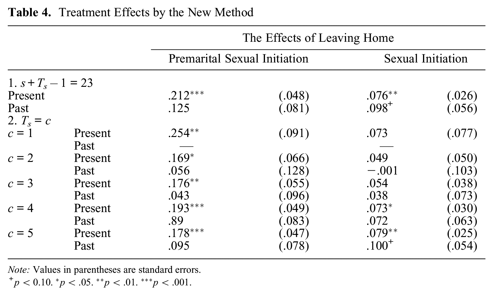
Table 4 presents the main analytic results from the conditional-incidence-rate model introduced in this article. I diagnosed several balancing tests for the estimation of propensity scores, and the equations I used met the criteria.³ Note that these tests involve only six selection equations for the six age categories of entry into treatment to assess the “present treatment” effects and 12 equations for six age categories of entry into treatment to assess the “past treatment” effect. Regarding the determinants of a competing event, getting married, preliminary analysis showed that leaving home does not have significant unique effects on the occurrence of marriage, which confirms that the assumption that the treatment variable does not affect censoring is adequate.

Table 4.

Treatment Effects by the New Method

		The Effects of Leaving Home
		Premarital Sexual Initiation		Sexual Initiation
1. s +T_s– 1 = 23
Present		.212***	(.048)	.076**	(.026)
Past		.125	(.081)	.098⁺	(.056)
2. T_s = c
c = 1	Present	.254**	(.091)	.073	(.077)
c = 1	Past	—		—
c = 2	Present	.169*	(.066)	.049	(.050)
c = 2	Past	.056	(.128)	−.001	(.103)
c = 3	Present	.176**	(.055)	.054	(.038)
c = 3	Past	.043	(.096)	.038	(.073)
c = 4	Present	.193***	(.049)	.073*	(.030)
c = 4	Past	.89	(.083)	.072	(.063)
c = 5	Present	.178***	(.047)	.079**	(.025)
c = 5	Past	.095	(.078)	.100⁺	(.054)

Note: Values in parentheses are standard errors.

p < 0.10. *p < .05. **p < .01. ***p < .001.

Analyses in Table 4 use two distinct specifications for periods covered in the calculation of the conditional-incidence rate. The first model is concerned with cumulative probability of event occurrence for the period from time of entry into treatment (varying from age 16 to age 21) to age 23. I use age 23 because in the sample analyzed here, more than 50 percent of subjects got married by age 23. The length of the period covered for those two models therefore varies from three to eight years among sample persons. The next five models are concerned with the effects of the present and past treatments on the cumulative probability of event occurrence for a fixed length of the period from entry into treatment. Estimates of the treatment effects are given for each of the five distinct time spans from one to five years, except no effect of the past treatment exists for the first period.

First, it is noteworthy that the conditional-incidence rate with only one period of observation after entry into treatment, where T_s = 1, is equal to the hazard rate for the period. However, the present treatment effects during the time span of one year in Table 4 (0.254 for premarital sexual initiation and 0.073 for sexual initiation in general) somewhat differ from the results of the first-period effect from the hazard rate model of Table 3 (0.262 for premarital sexual initiation and 0.122 for general sexual initiation). These differences are minor and may reflect differences between the ATT and the treatment effect based on the covariance analysis of the hazard rate model. Their standard errors are similar, and no difference exists regarding the significance of the two treatment effects between the two results.

Results in Table 4 show that leaving home positively affects the rate of premarital sexual initiation. This effect is particularly strong during the one-year period after leaving home, as indicated by a reduction in the present treatment effects for the time span of $c \geq 2$ , compared with the effect for a one-year time span (c = 1). This implies that leaving home not only increases the cumulative probability of experiencing premarital sexual initiation, but it also accelerates the timing of its occurrence by increasing the probability of event occurrence during the first 12 months after leaving home. The effect of the “past treatment” on the occurrence of premarital sexual initiation is consistently absent regardless of the time span of the cumulative-incidence rate. This implies that after the increase in the rate of premarital sexual initiation during one year after leaving home, there is no further effect of having left home on the incidence rate of premarital sexual initiation for the rest of the periods. On the other hand, the effect of leaving home is significant in the hazard rate model 2 of Table 3 not only for the first period after leaving home but for the later periods as well. Although this disagreement between the hazard rate model and the cumulative-incident-rate analysis may make the two seem contradictory, the cumulative-incidence rate starting from the second period reflects the consequence of event occurrences in the first period, whereas the hazard rate does not. Results from the incidence-rate model indicate there is no effect of having left home on the conditional survival probability of the occurrence of premarital sexual initiation from the second year after leaving home.

Regarding the effect of leaving home on sexual initiation in general, the results show that the present treatment effect is significant but weaker in magnitude than the effect on premarital sexual initiation. In particular, for the hazard rate model, the distinction between the first and later periods of treatment makes both effects nonsignificant. However, results for the analysis of the cumulative-incidence rate in Table 4 reveal a more complicated story: the present treatment effects are not significant for the shorter time span, up to three years after leaving home, but they gain significance for the time spans of four and five years. This is not due to an increase in the treatment effect with time span but due to smaller standard errors of the treatment effect for event occurrence in the longer time interval. In fact, the lack of statistical significance in the hazard rate model when we separate the treatment effect into those of the first period and later periods is simply a result of increases in the standard errors of the treatment effects. Similarly, the stronger significance of the treatment effect on sexual initiation in general in the incidence-rate model compared with the hazard rate model is not due to a difference in the size of the treatment effect, which is actually greater for the hazard rate model, but due to a smaller standard error of the treatment effect for the cumulative-incidence rate.

It is also worthwhile to compare the behavior of standard errors between two methods. First, comparing the standard error of the present treatment effect up to age 23 on the rate in Table 4 to the corresponding standard error of model 1 in Table 3, we see that the standard error is much smaller in Table 4 for both premarital sexual initiation and sexual initiation in general. The greater efficiency in the parameter estimates in Table 4 compared with those in Table 3 results from use of the cumulative conditional-incidence rate rather than the hazard rate in estimating the treatment effect on relative rates. For the conditional-incidence rate, subjects who experienced the event and those who experienced censoring after entry into risk remain in the denominator of the rate, but they do not for the hazard rate. It follows that for the hazard rate, the denominator of rates to be compared—the sample size of the treatment group and the control group in Table 2 for each treatment-entry cohort—is reduced as subjects experience the event or censoring and leave the risk set. But this does not happen for the incidence-rate model because the denominator of the rate remains the same throughout the observed time. Hence, when the event or censoring occurs for the majority of subjects by age 23, the rate estimates for higher ages are based on much smaller samples in the hazard rate model than in the conditional-incidence-rate model, leading to a greater standard error for the treatment effect for the former than for the latter.

Conclusions

This article proposes a semiparametric approach to estimation of the ATT on the conditional cumulative-incidence rate. The choice of modeling incidence rates rather than a hazard rate eliminates the problem of endogenous sample selection and the consequent bias in the MSM proposed by Robins et al. (2000) for a hazard rate model of a nonrepeatable event regarding the effect of past treatments. Similar to the original use of the IPT weighting method introduced by Rubin (1985), the method proposed in this article permits estimation of the ATT simply as the difference in average outcome between the treatment group and the IPT-weighted control group at each time of entry into treatment.

The choice of modeling the conditional-incidence rate and estimation of the treatment effect on the cumulative rate of event occurrence leads to the necessity of controlling for selection bias only once at time of entry into treatment for estimation of the present treatment effect and only twice for estimation of the past treatment effect, and thereby greatly simplifies the estimation and application of the IPT weights compared with use of the MSM. The modeling of the conditional-incidence rate rather than the hazard rate has the additional advantage of yielding smaller standard errors, especially for an event for which the majority of subjects leave the risk set of the hazard rate as time passes, because the incidence rate keeps subjects in the denominators of the rate regardless of event occurrences.

The new method introduced, however, changes the parameters of interest regarding the treatment effects, and they are not the same as parameters of the treatment effects in the hazard rate model. However, the availability of consistent test statistics for the test of the significance of treatment effects in the presence of unobserved population heterogeneity seems to be much more important than not having such a statistic.

Footnotes

Appendix A: A Note on the Fact that Censored Observations can be Treated as Event Nonoccurrence in Analysis of the Cumulative-Incidence Rate with the Effect of the Past Treatment

For estimation of the effect of Z(s) as the effect of “the past treatment,” I consider the following modified semiparametric conditional-incidence-rate model:

(A1)

\begin{matrix} \log (R_{i} (t | Z^{*} (s - 1) = 0, Y^{*} (s - 1) = 0, C_{si} (t) = 0)) = α_{s, t} + β_{s 1} δ_{t = s} Z_{i} (s) + β_{s 2} δ_{t > s} Z_{i} (s) \\ + β_{s + 1} Z (s + 1) + ϕ (V_{i} (s), X_{i} (s)) + U_{i}), for s \leq t \leq s + T_{s} - 1 . \end{matrix}

Here, as in the case of the model of equation (18), I assume that censoring depends only on V(s), X(s), and U and neither on Z(s) nor on Z(s+1). Note that V(s+1) and Y(s), both of which can be mediating variables for the effect of Z(s) on the outcome, are not controlled in equation (A1).

This modified model differs from the model of equation (18) in two respects. First, two effects of Z(s) are separated between the effect at time s and the effect at later times. Two Kronecker’s deltas, $δ_{t = s}$ and $δ_{t > s}$ , interacting with Z(s) represent this distinction. The coefficient $β_{s 1}$ reflects the effect of Z(s) on the outcome at time s, and the coefficient $β_{s 2}$ , which reflects the effect of Z(s) on the outcome at time s+1 and later, represents the past treatment effect of Z(s). Two parameters are separated in order not to impose any parametric interdependence between the effect of Z(s) on the outcome at time s and the past treatment effect. Second, this model adds to the model of equation (18) the effect of Z(s+1) because the past treatment effect is conceived as the effect of Z(s) on the outcome during the time of interval of [s+1, s+T_s– 1] when Z(s+1) = 0. Z(s+1) is thus the only mediating variable controlled in the model of equation (A1).

It follows that the cumulative joint rate of event occurrence and nonoccurrence over the time interval of [s+1, s+T_s– 1] for the treatment group becomes basically the same as equation (19), because Z(s+1) = 0 for this group, except that time aggregation needs to be made for the time interval of [s+1, s+T_s– 1] instead of [s, s+T_s– 1]. We can thus express the result as $\exp (β_{s 2}) Q$ , where Q indicates the common part of equations (19) and (20), except the joint rates are aggregated over the time interval of [s+1, s+T_s– 1]. Note that the denominator of the joint rate of event occurrence and censoring nonoccurrence does not change over time, and therefore we can divide their sum over time into any time segments.

For the control group, we consider the cumulative joint rate of event occurrence and censoring nonoccurrence separately for each given value of Z(s+1). Here, from the definition of weights $ω (v (s + 1), y (s))$ in equation (16), the weighted joint distribution of V(s), V(s+1), and Y(s) weighted by $ω (v (s)) ω (v (s + 1), y (s))$ not only preserves their joint distribution weighted by $ω (v (s))$ , that is, $f_{ω (z (s) ω (z (s + 1), y (s))} (V (s), V (s + 1), Y (s) | Z (s) = 0) = f_{ω (z (s))} (V (s), V (s + 1), Y (s) | Z (s) = 0)$ , but also weighting by $ω (v (s)) ω (v (s + 1), y (s))$ makes the joint distribution independent of Z(s+1). These characteristics hold when this joint probability densities of V(s), V(s+1), and Y(s) are summed over the values of Y(s) and the values of V(s+1) not commonly included in V(s). In addition, because of the definition of weights $ω (v (s))$ , $f_{ω (z (s))} (V (s) | Z (s) = 0) = f (V (s) | Z (s) = 1)$ also holds. It follows that

(A1)

\begin{matrix} f_{ω (z (s)) ω (z (s + 1), y (s))} (V (s) | Z (s) = 0, Z (s + 1)) = f_{ω (z (s))} (V (s) | Z ((s) = 0, Z (s + 1)) \\ = f_{ω (z (s))} (V (s) | Z (s) = 0) = f (V (s) | Z (s) = 1) . \end{matrix}

It follows from this that the weighted cumulative joint rate of the event occurrence and censoring nonoccurrence over the time interval of [s+1, s+T_s– 1] for the control group for a given value of Z(s+1) is equal to $\exp (β_{s + 1} Z (s + 1)) Q$ .

Hence, the ratio of the cumulative joint probability of the event occurrence and censoring nonoccurrence over the time interval of [s+1, s+T_s– 1] between the treatment group and the control group weighted by $ω (v (s)) ω (v (s + 1), y (s))$ becomes $\exp (β_{s 2} - β_{s + 1} Z (s + 1))$ . The difference in log rate between the treatment group and the control group becomes $β_{s 2}$ when Z(s+1) = 0. Hence, as in the case of the estimation of the present treatment effect, the effect of Z(s) on the rate ratio of the joint cumulative probability of event occurrence and censoring nonoccurrence becomes equal to the effect of Z(s) as the past treatment effect on the conditional-incidence-rate of model (A1). This also implies that we can treat censored observations equally with the case of event nonoccurrence for the period of [s+1, s+T_s– 1].

Appendix B: Stata Commands to Estimate the Present and Past Treatment Effects

Here, I provide STATA commands to estimate $β_{s}$ for both the present and past treatments for each given set of (s, T_s). The following notations are used for variable labels in the STATA commands:

The program assumes individual data from which subjects with either a treatment or an event occurrence prior to time s are already eliminated. Commands for the procedure described in the brackets [ ] are omitted.

ORCID iD

Kazuo Yamaguchi

Notes

Author Biography

Kazuo Yamaguchi is the Ralph Louis Professor of Sociology at the University of Chicago. His book Gender Inequality in the Japanese Workplace and Employment (Springer, 2019), uses propensity score methods for causal inferences and the decomposition analysis of inequality. In 2020, he was recognized as a Person of Cultural Merit by the Japanese government, which is an honor given annually to 20 people in the arts, sciences, and sports on Culture Day.

References

Barber

Jennifer S.

Murphy

Susan A.

Verbitsky

Natalya

. 2004. “Adjusting for Time-Varying Confounding in Survival Analysis.” Sociological Methodology 34:163–92.

Blossfeld

Hans-Peter

Hamerle

Alfred

Mayer

Kurl Ulrich

. 1989. Event History Analysis. Hillside, NJ: Lawrence Erlbaum.

Elwert

Felix

Winship

Christopher

. 2014. “Endogenous Selection Bias.” Annual Review of Sociology 40:31–53.

Flinn

Christopher J.

Heckman

James J.

1982. “New Methods for Analyzing Event Histories.” Sociological Methodology 1982:99–140.

Heckman

James J.

Singer

Burton

. 1982. “Population Heterogeneity in Demographic Models.” Pp. 567–98 in Multidimensional Mathematical Demography, edited by Land

K. C.

Rogers

New York: Academic Press.

Hernán

Miguel Angel

Brumback

Babette

Robins

James M.

2000. “Marginal Structural Models to Estimate the Causal Effects of Zidovudine on the Survival of HIV-Positive Men.” Epidemiology 11(5):561–70.

Huber

Peter J.

1964. “Robust Estimation of a Location Parameter.” Annals of Mathematical Statistics 35:73–101.

Huber

Peter J.

1967. “The Behavior of Maximum Likelihood Estimates under Nonstandard Conditions.”

Proceedings of the 5th Berkeley Symposium

1:221–33.

Laumann

Edward O.

Gagnon

John H.

Michael

Robert T.

Michaels

Stuart

. 1994. Social Organization of Sexuality. Chicago: University of Chicago Press.

10.

Morgan

Stephen L.

Winship

Christopher

. 2007. Counterfactuals and Causal Inference. Cambridge, UK: Cambridge University Press.

11.

Robins

James M.

Hernán

Miguel Angel

Brumback

Babette

. 2000. “Marginal Structural Models and Causal Inference in Epidemiology.” Epidemiology 11(5):550–60.

12.

Rosenbaum

Paul R.

Rubin

Donald B.

1983. “The Central Role of the Propensity Score in Observational Studies for Causal Effects.” Biometrika 70(1):41–55.

13.

Rosenbaum

Paul R.

Rubin

Donald B.

1984. “Reducing Bias in Observational Studies Using Sub-classification on the Propensity Scores.” Journal of the American Statistical Association 79:516–24.

14.

Rubin

Donald B.

1985. “The Use of Propensity Scores in Applied Bayesian Inference.” Pp. 463–72 in Bayesian Statistics, Vol. 2, edited by Bernardo

J. M.

De Groot

M. H.

Lindley

D. V.

Smith

A. F. M.

North-Holland, the Netherlands: Elsevier.

15.

Tuma

Nancy

. [1978] 1985. “Effects of Labor Market Structure on Job Shift Patterns.” Pp. 327–65 in Longitudinal Analysis of Labor Market Data, edited by Heckman

J. J.

Singer

Cambridge, UK: Cambridge University Press.

16.

Vermunt

Jeroen K.

1998. Log-Linear Models for Event Histories. Newbury Park, CA: Sage.

17.

Yamaguchi

Kazuo

. 1986. “Alternative Approaches to Unobserved Heterogeneity in the Analysis of Repeatable Events.” Sociological Methodology 16:213–49.

18.

Yamaguchi

Kazuo

. 2012. “Loglinear Causal Analysis.” Sociological Methodology 42:257–85.