
Abstract
The opportunities for understanding how treatment effects vary across different segments of the population have led to a rise in the use of quantile regressions for identifying unconditional quantile treatment effects (QTEs). However, existing quantile regression models fall into two categories: those that are unsuitable for identifying unconditional QTEs and those that often struggle with the complex data structures common in sociology and other social sciences. In particular, existing methods face difficulties with large data sets and high-dimensional fixed effects. The authors introduce a two-step approach to estimating unconditional QTEs, which is easy to use and aligns with the needs of sociologists. First, the treatment variable is decomposed into a systematic and random part, and then, the random variation in the treatment status is used as the sole independent variable in a quantile regression model. Through a series of simulations and three empirical applications, the authors provide strong evidence that the residualized quantile regression (RQR) approach provides approximately unbiased estimates of unconditional QTEs comparable with existing methods. Moreover, the RQR approach offers greater flexibility and enhances computational speed compared with existing models, and it can easily handle high-dimensional fixed effects. In sum, the RQR approach fills a pressing void in quantitative research methodology, offering a much-needed tool for studying treatment effect heterogeneity.
Keywords
Studying differences between groups has historically been akin to looking at differences in means. However, researchers increasingly turn to quantile regression models to get a complete view of how treatments affect outcomes (Koenker 2005). One advantage of quantile regression models over standard linear regression models is that we can study how differences between groups vary across the outcome variable’s distribution, allowing researchers to explore new types of research questions. Generally, whereas linear regression models enable us to examine how the average of the outcome differs between groups, quantile regression models allow us to study how quantile values differ (Firpo 2007). Thus, quantile regression models can be used to analyze how individuals prone to have high outcomes react differently to treatment than do individuals with low propensity; this is called unconditional quantile treatment effects (QTEs). We can, for example, investigate whether the motherhood wage penalty is more pronounced for women at the upper end of the wage distribution compared with women at the lower end (Killewald and Bearak 2014).
Historically, the conditional quantile regression (CQR) model, which builds on Roger Koenker and colleagues’ work in the mid-1970s, has been used to estimate quantile regression coefficients (Koenker 2017). CQR coefficients can be interpreted as unconditional QTEs whenever we do not need to include any control variables in our model (e.g., randomized treatment). However, unlike in linear regression models, including control variables changes the interpretation of the CQR coefficients, and they can no longer be interpreted as unconditional QTEs (Borgen, Haupt, and Wiborg 2023; Firpo 2007; Killewald and Bearak 2014; Rios-Avila and Maroto 2024; Wenz 2019). Therefore, solutions that allow the inclusion of control variables in quantile regression models while simultaneously preserving the coefficients’ interpretation as unconditional QTEs are being developed (Firpo 2007; Frölich and Melly 2010; Powell 2020).
This article adds to this growing literature by offering a new quantile treatment estimation method, called residualized quantile regression (RQR), which complements existing approaches. In his seminal article, Firpo (2007) proposed an elegant solution to estimate unconditional QTEs with a single binary treatment variable using a propensity score matching framework. However, the propensity score framework cannot be used with nonbinary treatment variables, and including fixed effects is problematic in a propensity score framework. Recently, Powell (2020) developed the generalized quantile regression (GQR) model that allows for nonbinary treatment variables. 1 However, this method is computationally demanding, with computational issues growing with the model’s complexity and the sample size. Thus, including high-dimensional fixed effects in large administrative data sets is challenging or practically impossible using the GQR model. As we will show, our estimation method can easily handle large data sets and complex model specifications.
The RQR model builds on the fact that a simple CQR model can estimate the unconditional QTE with a randomized treatment. In social sciences, assignment of the treatment status often rests on a selection process. However, under the assumption of selection on observables, the treatment assignment can be decomposed into a systematic part caused by the observed confounders and a random part. By using only the random part of the treatment assignment in a quantile regression model, we can straightforwardly estimate unconditional QTEs. More specifically, our approach involves a two-step method. First, we decompose the treatment variable into systematic and residual components. In most cases, a simple linear regression model, regressing the treatment on the observed confounders, will be sufficient, but other regression models can be used to account for the specific sorting patterns into treatment. The residuals derived from the first-step model can act as the as-if randomized treatment assignment. Next, the outcome variable is regressed on the residualized treatment variable using a CQR model with only the residualized treatment as the independent variable. Because the control variables purge the treatment of confounding in the first step, they are redundant in the second step. Thus, our approach serves as a straightforward solution to estimate unconditional QTEs in the presence of covariates.
The RQR model has several advantages over current QTE approaches, making it a valuable addition to the quantile regression toolkit. Its most significant contribution lies in its ability to incorporate high-dimensional fixed effects into the estimation of unconditional QTEs, a critical feature for identifying the motherhood wage penalty and numerous other treatment effects. Additionally, the estimation procedure is computationally efficient, the model allows for both binary and nonbinary treatment variables, and it is straightforward to implement the RQR model in all software that provides a package for CQR or linear programming. Borgen, Haupt, and Wiborg (2021) introduce the rqr and rqrplot Stata commands that estimate and plot RQR coefficients.
The RQR model belongs to a different class of models than the popular unconditional quantile regression (UQR) model (Firpo, Fortin, and Lemieux 2009). The distinction between these models is discussed in detail by Rios-Avila and Maroto (2024) and Borgen et al. (2023). Here, we briefly clarify their difference. The UQR model approximates the marginal effects of independent variables on unconditional quantile values through a two-step approach. First, the quantile values of the outcome distribution are reduced to a fixed set of binary outcome variables via the recentered influence function. Then, these binary outcome variables are regressed on the independent variables using separate linear regression models. The UQR model is often used to identify QTEs, but it was developed to infer how independent variables influence overall quantile values and should be applied cautiously when examining QTEs of binary variables (Borgen et al. 2023). Within the UQR framework, Firpo and Pinto (2016) offer a solution to derive QTEs by reweighting the outcome distributions. This approach is succinctly outlined in Rios-Avila and Maroto (2024), and Rios-Avila (2020) provides tools to estimate QTEs.
In the following, we start by defining the unconditional QTE. We then describe the RQR model in more detail. Last, we showcase the RQR model’s performance in data simulations and empirical applications on real data, comparing the RQR approach with other quantile regression approaches.
Unconditional QTEs
Ordinary least squares (OLS) and its estimation of average treatment effects (ATEs) is the main workhorse of quantitative empirical research, but scholars are increasingly turning to quantile regression models to estimate unconditional QTEs. The main attraction of unconditional QTEs is that it allows one to study treatment effect heterogeneity by individuals’ overall propensity to have high or low outcomes.
Because of their close resemblance, let us briefly define ATE before turning to QTEs. In the potential outcomes framework (Morgan and Winship 2015), the causal effect of a treatment for a single unit is defined as

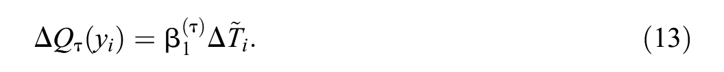
where

Likewise, if we know the whole distribution of the potential outcomes,

where
Whether unconditional QTEs differ from ATE depends on how the treatment influences the outcome (Hao and Naiman 2007). For example, suppose the treatment only shifts the outcome distribution’s location left or right, as shown in Figure 1A. If a treatment only induces a location shift, it has a similar effect on all units across the potential outcome distribution. In that case, the difference between the 10th, 50th, 90th, or any other percentile under the treatment (

Illustrating the difference between OLS and QTE when the treatment variable induces only a location shift (A) and when the treatment induces both a location and a scale shift (B).
Estimating QTE in Cases with and without Randomization
Because counterfactual observations cannot be directly observed, estimation of unconditional QTEs must be based on the comparison of outcome distributions for the treated and untreated. Several assumptions must be met for this comparison of realized outcome distributions to provide an unbiased estimate of the unconditional QTEs, as we will detail when introducing the RQR model below. One of the key assumptions is the rank preservation assumption. Another is that the treated and untreated must differ only randomly concerning the composition of other factors that influence the outcome (i.e., the unconfoundedness assumption). If this assumption holds, then we can use the outcome distribution of the treatment groups as the what-if potential outcome distributions under different treatment conditions.
It follows from this that estimating unconditional QTEs is effortless in the rare case where treatment assignment is truly randomized. In that case, the treatment status is independent of other factors influencing the outcome, and therefore independent of the potential outcomes. Thus, given a randomized treatment variable, we can ignore other influences and compare the distributions of the treated and untreated directly: one could calculate the quantile values among the treated and compare them with the corresponding quantile values among the untreated. The differences between these quantile values are the unconditional QTEs. Likewise, we can estimate these unconditional QTEs using a simple (conditional) quantile regression model without covariates (Koenker 2005).
However, treatment variables in the social sciences are typically not randomly assigned but involve selection processes. Therefore, in most cases, we want to add control variables or fixed effects to account for selection bias (Killewald and Bearak 2014). Even in randomized controlled trials, controls for baseline characteristics are often needed to ensure the estimates’ internal validity. Unfortunately, estimating QTEs in the presence of control variables is more complicated than estimating treatment effects in the OLS model.
To illustrate the complexity of estimating unconditional QTEs with control variables, let us consider an example. This example also underscores the differences between linear regression and quantile regressions, as well as between quantile regression models estimating conditional and unconditional QTEs. We take the motherhood wage penalty as a starting point and, for pedagogical purposes, consider a simple model that assumes selection on observables, as is common in motherhood wage penalty studies (Cukrowska-Torzewska and Matysiak 2020). Consider the structural model where individual i’s wages y depend on motherhood status MS, years of education E, and other (unmeasured) causal factors e:
In comparison, quantile regressions can be used to examine heterogeneity in terms of all factors influencing the outcome. Specifically, the CQR model estimates whether the effects of motherhood status differ according to unobserved factors that influence the outcome, that is, the rank of the residual
Studying conditional quantiles provides a unique way of estimating heterogeneity by unobserved factors influencing the outcome variable, making CQR a useful tool for examining heterogeneity by hard-to-observe characteristics. However, as highlighted in a number of studies (Borgen et al. 2023; Firpo 2007; Frölich and Melly 2010; Killewald and Bearak 2014; Wenz 2019), although comparing conditional quantile values efficiently accounts for selection on observables, it changes the interpretation of the coefficients. For example, instead of estimating treatment effects for units that, in the absence of the treatment, would have a high rank in the outcome distribution, the CQR model estimates effects on the basis of ranks conditional on the observed predictors. Women who have a high rank relative to others with the same education do not necessarily have an overall high rank. Furthermore, because the definition of high and low quantiles depends on the included independent variables, adding additional covariates will change the meaning of the estimated treatment effect.
Whereas CQR estimates effects on the basis of ranks conditional on the observed predictors, which means its coefficients have a conditional interpretation, scholars have developed approaches to translate CQR coefficients into their effect on overall marginal (or unconditional) quantiles. Notably, Machado and Santos Silva (2005) and Chernozhukov, Fernández-Val, and Melly (2013) provide methods that use CQR models to analyze counterfactual distributions. These methods, particularly Chernozhukov et al. (2013), aim to estimate and recover QTEs for settings involving binary treatments. This is achieved by linking CQR models to conditional distribution models, which are then integrated with covariate distributions to form counterfactual distributions.
Several approaches have also been developed to directly estimate unconditional QTEs in the presence of control variables (Firpo 2007; Frölich and Melly 2010; Powell 2020). Unlike the CQR model, QTE models attempt to estimate whether the effects of motherhood status differ according to all other factors that influence the outcome, both observed and unobserved. Let
This article adds a new model to this class of QTE models. We claim this new RQR model has several practical advantages over existing ones, especially in terms of flexibility to add high-dimensional fixed effects and computational speed. In the following section, we present the framework, followed by a discussion of the advantages relative to existing models.
The RQR Model
We introduce a two-step approach to identify QTEs where the treatment variable is purged of confounding in the first step, followed by a QTE estimation in the second step using a quantile regression model. The core building block of this two-step approach is the decomposition of the treatment variable into a systematic piece explained by the observed control variables and a piece orthogonal to the controls. The next subsection elaborates on this decomposition before providing more details about the RQR approach.
Decomposition of the Treatment Variable
Assuming selection on observables, the variation in treatment variable values is a function of confounding variables and other random factors. Let

We want to decompose the treatment variable
Consider the following data-generating process where

In this case, the confounder

using a simple linear model.
For our purpose, the main takeaway point is the decomposition of the treatment variable into a piece explained by

Given a correctly specified model, the (treatment) residuals are mean independent of the confounder
A Two-Step Approach to Estimating QTEs
We propose to estimate QTEs using the following two-step approach:
Step 1: Decompose the treatment variable into a piece explained by the observed control variables and a residual piece.
Step 2: Regress the outcome variable on the residualized treatment variable using the CQR algorithm.
Several assumptions must be met for this two-step estimator to identify QTEs. The most important assumption is the unconfoundedness assumption, which loosely states that all variables affecting the treatment and the outcome (i.e., confounders) are observed and that the treatment selection is correctly specified. More specifically, we assume the potential outcomes are independent of the treatment
Assumption 1 (unconfoundedness):
This unconfoundedness assumption is fundamentally nonparametric, meaning it does not impose any specific functional form on the relationship between the potential outcomes, treatment, and observed control variables. Although nonparametric by nature, identification of treatment effects based on this assumption typically requires selection of a specific parametric model. Given that this parametric model adheres to the unconfoundedness assumption, a crucial point is that it implies the conditional independence of potential outcomes from the treatment residuals:
In fact, the conditional independence of the residuals from the potential outcomes follows from the unconfoundedness assumption. That is, once the treatment is decomposed into
However, it is crucial to note that assuming the potential outcomes are independent of the treatment given the covariates (i.e., assuming selection on observables) is a strong assumption, particularly within a parametric setting. Similar to Powell’s (2020) GQR model and Firpo’s (2007) propensity score approach, selection on unobservables would bias the estimates of QTEs.
The unconfoundedness assumption and the fact that the treatment is residualized before estimating the quantile regression model are the main departures from the CQR model. Thus, other conditions required in the CQR model, covered in detail by Koenker (2005), also apply to the RQR model, such as the assumption of no quantile crossing (He 1997) and a continuously distributed outcome variable (Machado and Santos Silva 2005). Let Y be a continuous random variable with the cumulative distribution function (CDF) of Y defined as
Assumption 2 (CDF is strictly monotonically increasing):
Additionally, we invoke the rank invariance assumption for the treatment effects to be interpreted as individual-level QTEs. The rank invariance assumption is assumed in all quantile regression models that attempt to identify individual-level QTEs (Firpo 2007; Koenker 2005; Powell 2020), and prior work has developed approaches for testing rank invariance or rank similarity (see below) (Dong and Shen 2018; Frandsen and Lefgren 2018; Kim and Park 2022). Consider the binary treatment variable
Assumption 3 (rank invariance assumption):
The rank invariance assumption is strong, and a violation of this assumption prevents the estimates from being interpreted as individual-level QTEs. However, if the weaker rank similarity assumption holds, the RQR estimates may still have a meaningful interpretation. The rank similarity relaxes the rank invariance assumption by allowing for random deviations or “slippages” in ranks under the treatment and control conditions (Dong and Shen 2018). Specifically, rank invariance is the condition where an individual’s potential rank with or without treatment remains the same, whereas rank similarity requires only that the potential ranks have the same conditional distribution when conditioned on specific observed and unobserved determinants of the common rank level. Formally, rank similarity is defined as the condition that
Estimation of the RQR Model
The RQR model consists of a two-step approach, where the first step isolates as-if variation in the treatment (i.e., treatment residuals). Achieving this requires a correctly specified first-step model, including correctly specifying the control variables and choosing the appropriate link function. Choosing the correct causal model, including what constitutes potential confounders, should be specified on the basis of know-how of the field (Morgan and Winship 2015; Pearl 2009). For example, not all covariates correlated with the treatment should be included, as highlighted by discussions on bias amplification of near-instrumental variables (Myers et al. 2011; Pearl 2011) and pretreatment collider variables (Elwert and Winship 2014). However, with a given set of covariates, and building on specification tests such as Ramsey’s (1969) reset test and Pregibon’s (1980) link test, we propose an F-test to jointly test whether there are unmodeled interactions or higher order terms among our covariates (see part C in the online supplement).
Concerning the choice of first-step estimator, the general framework developed here does not specify the approach used for decomposing the treatment variable in the first step. The first-step estimator should be chosen on the basis of whether it allows for satisfying the unconfoundedness assumption. For example, it is well known that with a binary treatment variable and common support problems, parametric models such as linear regression may perform poorly, and dropping observations out of support may be needed (Lechner and Strittmatter 2019). Thus, when the treatment is binary, there are benefits of using a logit or probit model to check common support and trim observations before performing the decomposition on the basis of the predicted probability of being treated from a logit model with common support. However, in most applications where we proceed under the assumption of selection on observables, a linear regression model offers a convenient first step to estimate
As detailed above, under selection on observables and a correctly specified model, the first step purges the treatment variable of confounding, allowing us to use the residuals as an as-if randomized treatment variable in the second step. Thus, residualization of the treatment allows the exclusion of control variables in the second step under an additive conditional quantile condition,
In the second step, linear programming methods are used to estimate coefficients. 2 The algorithm is only briefly described here; details can be found in Koenker (2005) and Hao and Naiman (2007). Known as the method of minimum absolute deviations, the QR estimator finds the coefficients that minimize the sum of weighted absolute residuals:

where

Note that in this second-step regression, the constant term rarely has a sensible interpretation; it is the predicted quantile value of the outcome when the treatment residuals are zero. Furthermore, by construction, there is a mechanical association between the residuals
To elucidate why

where quantile-specific predicted outcomes are defined as

and the outcome residuals

Units are sorted based on whether their observed outcomes
Under assumption 1 and the additive conditional quantile condition, differences observed in the quantile-specific predicted outcome can be attributed to differences in treatment residuals:
That is, the mapping from
The adjustment-based two-step RQR approach provides asymptotically unbiased estimates of unconditional QTEs given that the unconfoundedness assumption holds. However, it is important to emphasize that the assumption of unconfoundedness is strong. Unobserved confounders or a misspecified model will bias RQR coefficients, similar to the case in other adjustment-based quantile regression models, including other QTE models, the UQR model, and the CQR model, as well as in linear regression models and propensity score matching approaches. An advantage of the RQR model is that we can include fixed effects to adjust for time-invariant unobserved confounders, in which case only failure to measure and correctly specify time-variant confounders is of concern (Allison 2009).
Inclusion of Fixed Effects
The inclusion of fixed effects constitutes a major challenge in nonlinear regression models, such as quantile regressions, because of the issue of the incidental parameter problem (Lancaster 2000). Several solutions to this problem have been developed within the CQR literature (Canay 2011; Koenker 2004; Machado and Santos Silva 2019; Powell 2022; Rios-Avila, Siles, and Canavire-Bacarreza 2024), including how to handle fixed effects without altering interpretation of the estimates (Powell 2022), but there have been fewer developments concerning the inclusion of fixed effects within the class of estimators that identify unconditional QTEs. A notable exception is Rios-Avila (2020) and Rios-Avila and Maroto (2024), which suggest unconditional QTEs of binary treatment variables can be estimated by combining the UQR model with a reweighting strategy based on inverse probability weights. However, although fixed effects are easy to include in the standard UQR framework, the estimation of QTE via a reweighting of the UQR model with fixed effects remains an open question, as argued by Rios-Avila and Maroto (2024). We supplement this literature by suggesting an alternative approach to include fixed effects.
In the RQR model, fixed effects can be included in the first-step regression, along with the other control variables, to ensure the potential outcomes are independent of the treatment. 4 Within the CQR literature, two-step estimators have been suggested to address the issue of the incidental parameter problem (e.g., Canay 2011; Machado and Santos Silva 2019; Rios-Avila et al. 2024). However, as these strategies aim to identify conditional QTEs, they differ from the approach suggested in the RQR model. For example, Canay (2011) assumes the fixed effects are location shifters and demean the outcome variable, before using CQR on the demeaned outcome variable. In contrast, the RQR model partials out the fixed effects from the treatment variable, and then uses a QR estimator with the demeaned treatment variable and the original (not demeaned) outcome variable. Two-step approaches, such as the one suggested in the RQR model, alleviate the incidental parameter problem but do not necessarily fully solve for it in all scenarios, particularly when the number of observations within each cluster is small and fixed (Canay 2011; Lancaster 2000; Machado and Santos Silva 2019; Rios-Avila et al. 2024). Note also that regarding the fixed effects in the RQR model, it is not the indicators themselves, but the unobserved confounders they represent, that contribute to satisfying the unconfoundedness assumption.
Inference
In various quantile regression models, estimation of standard errors using the bootstrap procedure (Hao and Naiman 2007; Mooney and Duval 1993) is preferred over the asymptotic procedure, including in the CQR model (Hao and Naiman 2007; Koenker and Hallock 2001), the propensity score QTE (PS-QTE) model (Firpo 2007), and the UQR model (Firpo et al. 2009). Estimating the asymptotic variance of quantile regression coefficients is notoriously challenging, as it depends on the unknown density of the dependent variable, and conclusions may be sensitive to the choice of kernel and bandwidths (Chernozhukov et al. 2013; Chernozhukov, Fernández-Val, and Melly 2022; Hagemann 2017; Koenker 2005; Powell 2020). Furthermore, simulation studies show that quantile regression inferences based on analytic standard errors perform worse than bootstrapping procedures (Chernozhukov et al. 2022; Hagemann 2017). Finally, providing analytic standard errors for testing differences of coefficients across quantiles is practically impossible (Hao and Naiman 2007), and bootstrapping or other simulation methods are therefore needed to test those types of hypotheses.
Bootstrapping within quantile regression models is computationally demanding (Fortin, Lemieux, and Firpo 2011), but this limitation can largely be circumvented by using the fast quantile regression algorithms provided by Chernozhukov, Fernández-Val, and Melly (2020). Thus, to provide valid inference, we propose to estimate standard errors in the RQR model using a bootstrap procedure, in which steps 1 and 2 described above are bootstrapped. Bootstrapping means randomly drawing M resamples of size N with replacements from the original data sample. In each resample, a decomposition of the treatment variable is followed by an estimation of the quantile regression coefficients using the as-if randomized treatment variable. The standard deviations of the estimated coefficients are the standard errors of the RQR coefficients.
As noted above, the bootstrapping procedure also provides a solution to testing differences of coefficients across quantiles. With nonparametric quantile regression, we often want to know whether the effect of some independent variable differs across quantiles. Eyeballing overlapping confidence intervals (CIs) is often informally used for this purpose, but it provides a too-conservative test and increases the risk for type 2 error (Greenland et al. 2016). The bootstrapping procedure is a solution to this eyeballing fallacy in quantile regressions (Hao and Naiman 2007). Consider the case of comparing quantile regression coefficients at the 10th (
Comparisons with Other Methods
The RQR model has several benefits compared with other quantile regression approaches. First, including high-dimensional fixed effects in the RQR model is straightforward. Like other control variables, fixed effects are included exclusively in the first step to account for confounding. After obtaining the treatment variable’s residuals (first step), we can estimate the unconditional QTE using the quantile regression model with the residualized treatment and the outcome variable (second step). In contrast, including high-dimensional fixed effects in the propensity score framework derived in Firpo (2007) is not only computationally burdensome but also potentially problematic because of the logistic regression model in the first step. In Powell’s (2020) GQR model, fixed effects can be included as information to construct the counterfactual distribution without treatment status (i.e., “proneness variables”); however, that computationally intensive solution is unfeasible with high-dimensional fixed effects.
Second, the RQR model is computationally efficient. The advent of big data and complex model specifications has made computational efficiency crucial in all regression models, but even more so in quantile regression models, where regressions are repeated at multiple quantiles and bootstrapping is needed for inference. The computational burden of quantile regressions may discourage researchers from using this approach (Chernozhukov et al. 2022; Fortin et al. 2011). When unconditional QTEs are estimated across multiple quantiles using the RQR model, one only needs to residualize the treatment variable once, making the estimation procedure more efficient and less computationally demanding. Furthermore, the computational time can be reduced considerably by applying newly developed quantile regression algorithms (Chernozhukov et al. 2020, 2022). As an illustration, consider the QTEs in Figure 3, discussed in detail below. Even with this undemanding model specification, the GQR model takes 20 times longer to run than the RQR model (for replication files, see part K in the online supplement).
Third, unlike the propensity score framework (Firpo 2007), the RQR approach extends to continuous treatment variables. Both binary and continuous treatment variables can be included in RQR without altering the coefficients’ interpretation or changing the estimation procedure. Although we can estimate QTEs of nonbinary treatment variables using the GQR model, that model cannot include fixed effects, as mentioned above.
Additionally, there are several minor benefits of the RQR approach. A fourth advantage is that the RQR framework can draw on the already extensive literature on CQR, including models to estimate parametric quantile regression (Frumento and Bottai 2016), methods to deal with count data (Machado and Santos Silva 2005), and fast algorithms (mentioned above). Finally, it is straightforward to implement the RQR estimator in all software that provides a package for CQR or linear programming, which makes it accessible to most researchers. 5
However, like GQR, the RQR estimates lack meaningful interpretation when the rank similarity assumption is violated. Although a weaker condition than rank invariance, rank similarity is still a strong assumption, and the propensity score matching approach developed by Firpo (2007) has the advantage of being interpreted as differences between quantiles of the marginal distributions of potential outcomes, regardless of whether the rank invariance or rank similarity assumptions hold or not. Therefore, the propensity score matching approach is preferred over RQR (and GQR) if rank similarity is violated and researchers are interested in comparing marginal distributions rather than individual-level QTEs.
Data Simulations
Data-Generating Process
In this section we use Monte Carlo simulations to compare the RQR model’s performance to other quantile regression approaches. We begin with fairly undemanding simulation scenarios before turning to more complex ones (results are presented Parts B–J in the online supplement). The data simulations in the main text consist of running 10,000 draws of N = 2,000 for two simulation scenarios. In both simulation scenarios, we have a continuous outcome variable
More specifically, in scenario 1, we begin by randomly assigning 25 percent of the sample the value 1 on the binary control variable

Finally, we allow the strength of the treatment variable (

The setup in scenario 2 is similar, except the conditional probability of being treated depends on
We estimate quantile regression coefficients using six different quantile regression models for each of the 10,000 draws and in each of the two simulation scenarios. Four of these estimation strategies identify unconditional QTEs, and their coefficients should, therefore, be nearly identical: the RQR method introduced in this article, Firpo’s (2007) PS-QTE approach, Powell’s (2020) GQR approach, and Rios-Avila’s (2020) reweighted UQR model, which we call UQR-QTE. The last two strategies are the CQR model (Koenker 2005) and the UQR model (Firpo et al. 2009), which we include because they are popular quantile regression methods. The RQR coefficients may differ from the CQR and UQR coefficients, which identify conditional QTEs and unconditional partial effects. All models are run with the treatment variable
Main Simulation Results
The main simulation results are shown in Table 1 and Figure 2. The reported
Average Differences between Estimated Regression Coefficients and the True QTE (

Note: Data simulation is performed in Stata 16.0; files to replicate the results are available in part K in the online supplement. CQR is the conditional quantile regression model (Koenker 2005) estimated using the qreg command; RQR is the residualized quantile regression model introduced in this article; PS-QTE is the propensity score framework of Firpo (2007) estimated using the ivqte command (Frölich and Melly 2010); GQR is the generalized quantile regression (Powell 2020) estimated using the genqreg command; UQR-QTE is the reweighting approach of the UQR model suggested by Rios-Avila (2020); and UQR is the unconditional quantile regression model (Firpo et al. 2009) estimated using the rifreg command. QTE = quantile treatment effect.

Average differences between estimated regression coefficients and the true QTE (
As expected, all four QTE models yield coefficients that approximate the true QTE across the outcome distribution, with the bias ranging from 0.001 to 0.005 in most cases. The differences between simulation scenario 1 (where there is no confounding) and simulation scenario 2 (where conditioning on
This article’s data simulation is not a comprehensive comparison of different QTE models. However, we note a few differences between the three QTE models in this setup. First, the bias is marginally lowest in the PS-QTE approach, followed by the RQR model, the UQR-QTE model, and finally, the GQR model (see Table 2). The average of the absolute value of the bias across the 19 quantiles is nearly identical at the third decimal in scenario 1. In scenario 2, the PS-QTE, RQR, and GQR models’ biases are 0.002, 0.003, and 0.005. Second, the standard deviations across the draws are 7 to 8 percent lower in the RQR and GQR models than in the PS-QTE and UQR-QTE models in scenario 2 (and indistinguishable in scenario 1). All in all, the differences between the QTE models are trivial in this simulation setup.
Average of the Absolute Values of the

Note: In each of the 10,000 draws, the average coefficient (
The QTE models’ coefficients differ from the CQR and UQR coefficients in both simulation scenarios. Let us start with the CQR results. As noted above, the difference between the CQR coefficients and the true QTE should not be interpreted as a bias, as the CQR model estimates conditional quantile value differences. As Figure 2 shows, the CQR coefficients differ in scenarios 1 and 2, despite the underlying unconditional QTE being the same in both scenarios. In fact, including the observed control variable
The unconditional partial effects, estimated using Firpo et al.’s (2009) UQR model, also differ considerably from the unconditional QTEs. Moreover, the UQR coefficients differ in scenarios 1 and 2, even though the underlying QTEs are the same. The differences between the QTE models (RQR, GQR, PS-QTE, and UQR-QTE) and the UQR model illustrate that the standard UQR model does not identify QTEs, although it is widely used in the literature for that purpose (Borgen et al. 2023). Thus, if the UQR model is used to examine unconditional QTEs of binary variables, one should use the reweighting approach (i.e., UQR-QTE).
Supplementary Simulation Scenarios
We supplement the simulation scenarios in the main text with a broader set of simulations in Parts B to J in the online supplement, including three simulation scenarios where the RQR model fails to identify the target estimand. We discuss these results briefly here, with more information included in the online supplement. First, part B in the supplement varies the distribution of the treatment, the structure of the QTE, and the skewness of the outcome distribution. Specifically, we simulate data with a binary treatment variable (as in the main text), a treatment variable with a uniformly distributed random component, and a treatment variable with a normally distributed random component. We also distinguish between three structures on the QTEs: constant, quadratic, and cubic. Finally, we allow the outcome’s residual distribution to be either normal or right skewed. The results in all 18 simulation scenarios align with the results discussed above: RQR provides approximately unbiased estimates of the unconditional QTEs given a correctly specified first step.
Second, part C in the online supplement simulates data where confounders interact and have a quadratic effect on the treatment. We show that incorrectly specifying the treatment selection results in biased estimates of the QTE. However, such misspecification can, in some cases, be detected using a specification test, as illustrated by the example in the supplement. Moreover, when interactions and quadratic effects are correctly specified, the RQR model provides approximately unbiased estimates of the QTEs.
Third, part D in the online supplement provides an example where the confounder’s effect on the treatment is allowed to vary randomly. For some individuals, the confounder strongly influences the treatment values, whereas it has no effect on others. (As a result, the variance of the treatment residuals increases as a function of the confounder.) We find that the RQR model provides approximately unbiased QTE estimates in this scenario.
Fourth, part E in the online supplement simulates data where the variance of the treatment is a function of the confounder. We find that the RQR model provides approximately unbiased estimates in a scenario where the variance of the treatment residuals is a function of the confounder.
Fifth, part F in the online supplement simulates data where the confounder has a curvilinear effect on the outcome and a scenario where the confounder has a QTE. Again, the RQR model provides approximately unbiased estimates in these simulation scenarios.
Sixth, part G in the supplement simulates panel data where there is a time-invariant unobserved confounder. Whereas other QTE approaches fail in such a scenario, we show that we can use the RQR model to identify approximately unbiased QTEs using a fixed effects estimator.
Finally, the last three supplements show simulations where the RQR model (and other QTE models) fails to identify QTEs. Part H simulates data where the rank invariance assumption is not met. Rank invariance means that individuals’ ranks in the potential outcome distributions remain the same irrespective of their treatment. Without invoking this assumption, QTEs cannot be interpreted as treatment effects for individuals located in different parts of the distribution. The supplement shows that RQR provides biased individual-level QTE estimates when rank invariance is not met, as do the GQR, PS-QTE, and UQR-QTE models. Next, part I illustrates how the RQR model fails to identify QTEs in the presence of quantile crossing, along with the GQR model. Finally, the CQR algorithm requires the uniqueness of quantiles (Firpo 2007), which is not satisfied with a discrete outcome variable (Machado and Santos Silva 2005). Part J shows that the RQR model struggles with discrete outcome variables, and it struggles more than the GQR model in the specific example included. However, the supplement also shows that the jittering approach of Machado and Santos Silva (2005) can be used to solve the problem.
Empirical Applications
After demonstrating the approximate unbiasedness of the RQR in various simulation scenarios where the identifying assumptions are met, we turn to real data applications. Our goal here is to benchmark RQR against established QTE estimators under comparable specifications, not to claim causal identification. In these applications, the true causal effects are unknown and identification is not guaranteed, because assumptions such as unconfoundedness and rank invariance may not hold and because of issues related to overcontrol. We compare estimated coefficients across methods to assess whether RQR recovers the same unconditional quantile contrasts in practice as established QTE estimators. Generally, similar coefficients support RQR’s performance relative to established estimators, although coefficients may differ somewhat because of sampling variability and differences in specifications or assumptions.
Current Population Survey
This section illustrates the RQR model using the Outgoing Rotation Group supplement of the Current Population Survey to study the effects of union status on men’s wages. We again highlight the quantile regression models’ differences. Union wage effects served as a motivating example in Firpo et al.’s (2009) UQR article, which has become popular in studies of QTEs (Borgen et al. 2023). Firpo et al. (2009) demonstrate that UQR coefficients differ from CQR coefficients. Here, we use the union wage effects example to showcase that RQR coefficients differ from UQR (and CQR) coefficients but not GQR, PS-QTE, or UQR-QTE coefficients. 7
Convincingly, differences between estimated union wage effects using QTE models are negligible; RQR, GQR, PS-QTE, and UQR-QTE coefficients decrease similarly, from about 0.40 at the 5th quantile to −0.10 at the 95th quantile (Figure 3). Concerning computational speed, less than a minute is needed to estimate the RQR coefficients on a standard laptop when using the fast quantile regression algorithms provided by Chernozhukov et al. (2020). The PS-QTE model takes more than five times longer to run, and the GQR model 20 times longer. The union wage effects are estimated with controls for age, education, marital status, and race. These control variables may not be sufficient to account for confounding; however, as potential bias is similar across models, the model specification allows us to compare RQR with the other quantile regression approaches.

Cross-sectional effects of union status on log wages for full-time working men in the 1983 to 1986 Outgoing Rotation group supplement of the Current Population Survey (N = 251,153).
Figure 4 compares RQR coefficients with UQR and CQR coefficients. For completeness, we also include the UQR-QTE coefficients. Two main results stand out in the cross-sectional analysis in Figure 4A. First, although the RQR and CQR models’ estimated union wage effects are monotonically declining across the outcome distribution, the gradient is steeper in the RQR model. The RQR coefficients are larger at the bottom of the wage distribution, before falling and eventually reaching a substantial adverse effect at the top. This finding highlights the difference between conditional and unconditional QTEs, as others have previously discussed (see Firpo 2007; Killewald and Bearak 2014; Porter 2015; Wenz 2019). Second, the UQR coefficients differ from the RQR coefficients, especially in the bottom fifth of the wage distribution. The reason is that Firpo et al.’s (2009) UQR model identifies UQPE rather than unconditional QTE.

Effects of union status on log wages for full-time working men in the 1983 to 1986 Outgoing Rotation group supplement of the Current Population Survey (N = 251,153).
In Figure 4B, we estimate union wage effects with household fixed effects. Including high-dimensional fixed effects in the RQR model is straightforward; fixed effects are treated as any other control variable and included only in the first step. After obtaining the treatment variable’s residuals, unconditional QTEs can be estimated by regressing the outcome on the residualized treatment in a quantile regression model. Fixed effects can also, with ease, be included in the UQR model (Borgen 2016; Rios-Avila 2020). However, as it is challenging in the CQR model (for one approach, see Machado and Santos Silva 2019), and estimation of QTE via UQR with fixed effects remains an open question (Rios-Avila and Maroto 2024), Figure 4B compares the RQR and UQR-QTE coefficients solely with those of UQR. In the union example, the estimated within-household treatment effects are generally lower than the cross-sectional estimates, especially at the bottom of the wage distribution. However, the overall trend is similar in the cross-sectional estimate (Figure 4A) and the fixed effects estimate (Figure 4B).
Norwegian Register Data
We use Norwegian register data in the following example, which largely alleviates issues caused by imprecise coefficients in small samples. Figure 5 looks at associations between 8th-grade standardized test scores and birth order, birth month (i.e., relative school-starting age), immigrant background, gender, school socioeconomic status, and parental earnings, where all independent variables are estimated controlling for the other independent variables in the graph. We show coefficients of all variables to illustrate the method across variables with different types of distributions. The four different QTE models provide nearly identical estimates for five of six variables. Importantly, this is the case despite the treatment effects having completely different effects across the outcome distribution. This result mirrors the findings in part B in the online supplement, where we use data simulations to show the RQR model can handle different treatment structures.
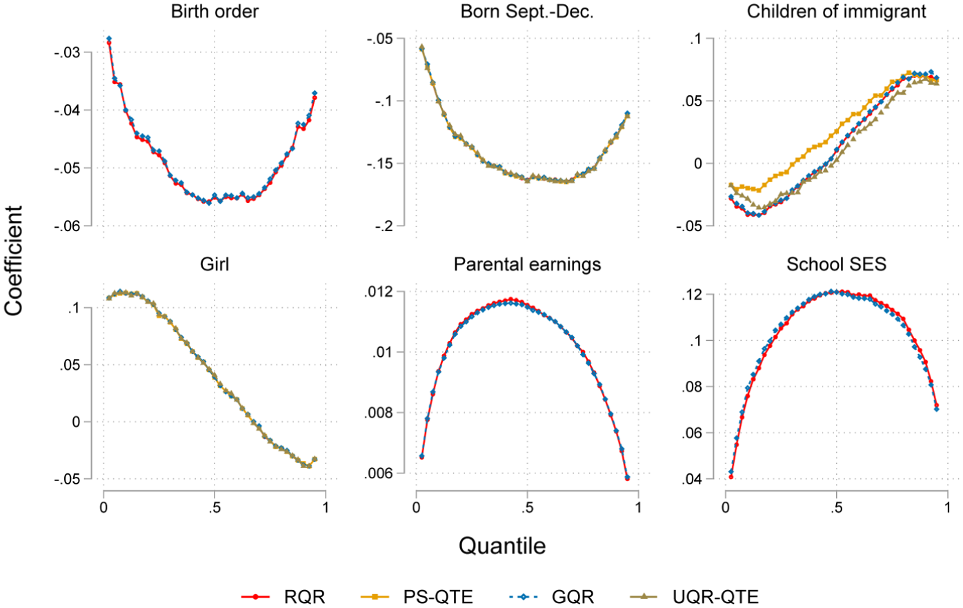
Comparing RQR, GQR, PS-QTE, and UQR-QTE coefficients on eighth grade standardized test scores in Norwegian register data (N = 480,264).
The exception is the variable children of immigrants, where the PS-QTE approach differs somewhat from the RQR, GQR, and UQR-QTE models. However, this difference does not warrant concern; rather, it showcases the well-known fact that regression and matching approaches may differ in some scenarios, despite identifying the same estimand. In this case, the inverse probability weighting matching approach also provides a different estimate of the ATE than does the classical OLS model (not shown).
National Longitudinal Survey of Young Working Women
As a final example, we use a subsample of the National Longitudinal Survey, containing panel data on 4,711 working women 14 to 26 years of age in 1968 from 1968 to 1988. The outcome is log wages, and as in Figure 5, we show coefficients for all independent variables. Although the smaller sample size results in noisier coefficients, we clearly see that the GQR, RQR, PS-QTE, and UQR-QTE coefficients resemble each other, irrespective of the type of independent variable (binary or metric) and the structure of treatment effects across the distribution (see Figure 6). 8

Comparing RQR, GQR, PS-QTE, and UQR-QTE coefficients on log wages in a subsample of the National Longitudinal Survey (N = 3,956).
Finally, Figure 7 illustrates the bootstrapping procedure to test differences of coefficients across quantiles. The figure uses a heat plot to show pairwise statistical significance across quantiles for the age variable.

Heat plot of p values to compare differences of age coefficients across quantiles on the basis of residualized quantile regression coefficients from Figure 6.
Discussion and Conclusions
Identification of unconditional QTEs has become increasingly popular within social sciences; however, contrary to popular belief, current methods to identify unconditional QTEs are incomplete. Firpo (2007) proposed a solution to estimate unconditional QTEs with a single binary treatment variable using a propensity-matching framework. Powell (2020) developed the GQR model that extends to nonbinary treatment variables. However, none of these approaches easily allows for high-dimensional (additive) fixed effects. Although a solution to estimate QTEs via UQR has been developed (Firpo and Pinto 2016; Rios-Avila 2020) and fixed effects are easy to include in the standard UQR framework (Borgen 2016; Rios-Avila 2020), estimation of QTE via UQR with fixed effects remains an open question (Rios-Avila and Maroto 2024).
This article fills a gap in the literature by introducing a straightforward framework to estimate unconditional QTEs of both continuous and binary treatment variables in the presence of covariates and high-dimensional fixed effects, called RQR. The main advantage of the RQR model compared with other QTE models is that fixed effects can be included, which is a common workhorse in causal modeling, as exemplified in the literature on motherhood and fatherhood wage penalties (Cooke 2014; England et al. 2016; Killewald and Bearak 2014). Although studies have highlighted that the fixed effects modeling strategy is not a panacea for causal inference (Imai and Kim 2021)—because of issues such as time-varying effects of time-invariant confounders (Ren and Allison 2025), potentially limited external validity (Hill et al. 2020; Lancaster 2000), and challenges related to variation in treatment timing in difference-in-difference models (Goodman-Bacon 2021)—it remains a powerful tool for identifying causal effects.
Furthermore, the RQR model can draw on the already extensive literature on CQR, is easy to implement in all software that provides packages for CQR or linear programming, and is computationally efficient compared with other quantile regression models. With better access to large-scale data and more complex model specifications, the computational burden may discourage researchers from using quantile regressions. The RQR model’s computational time can be reduced considerably by applying newly developed quantile regression algorithms (Chernozhukov et al. 2020, 2022), making it substantially faster than current QTE approaches. Borgen et al. (2021) provide a Stata command that exploits these fast algorithms.
This article introduced a new framework for estimating unconditional QTEs and provided strong evidence that it produces coefficients similar to other QTE models. We suggested using OLS in the first-step regression to deconfound the treatment variable; however, future research should explore other first-step regressions, especially with binary treatment variables. Furthermore, statistical inference and estimation of RQR standard errors need more work. Bootstrapping the two-step procedure seemingly provides sound standard errors, as the 95 percent bootstrapped CIs in our data simulations have coverage rates of 94.34 percent (normal-approximation bootstrap CIs), 95.26 percent (percentile bootstrap CIs), and 94.52 percent (bias-corrected bootstrap CIs) (see Figure A4 in the online supplement). Future work should systematically test the performance of various bootstrap procedures in different simulation scenarios. Additionally, the interpretation of RQR coefficients as individual-level QTEs depends on the rank similarity assumption. Approaches for testing rank similarity have been developed (Dong and Shen 2018; Frandsen and Lefgren 2018; Kim and Park 2022), but more research is needed to test rank similarity within the RQR framework. With binary treatment variables, the propensity score matching approach developed by Firpo (2007) may be preferable, as the estimated treatment effects have a meaningful interpretation even when the rank similarity assumption does not hold. Finally, the current article only dealt with the case of selection on observables. The RQR framework should be developed to allow the identification of an endogenous treatment variable’s QTEs via instrumental variable estimation.
Supplemental Material
sj-docx-1-smx-10.1177_00811750261450139 – Supplemental material for A New Framework for Estimation of Unconditional Quantile Treatment Effects: The Residualized Quantile Regression (RQR) Model
Supplemental material, sj-docx-1-smx-10.1177_00811750261450139 for A New Framework for Estimation of Unconditional Quantile Treatment Effects: The Residualized Quantile Regression (RQR) Model by Nicolai Borgen, Andreas Haupt and Øyvind Wiborg in Sociological Methodology
Footnotes
Acknowledgements
Earlier versions of this article were presented at the 2021 International Sociological Association RC28 Spring Meeting in Turku, Finland, the 2022 DAGStat Conference in Hamburg, Germany, the Social Inequalities and Population Dynamics group’s seminar at the University of Oslo in 2021, and the EQOP seminar at the University of Oslo in 2021. We thank participants for their comments and suggestions.
Authors’ Note
The authors used Refine and GPT UiO (powered by OpenAI’s GPT models) to assist with presubmission consistency checks. Grammarly and GPT UiO were used for language editing.
Funding
The authors disclosed receipt of the following financial support for the research, authorship, and/or publication of this article: The preparation of this article was supported by funding from the European Research Council (grants 818425 and 101115949) and was partially supported by the Research Council of Norway through its Centres of Excellence scheme (grant 331640). The register data were made available by Statistics Norway. Views and opinions expressed are those of the author(s) only and do not necessarily reflect those of the European Union or the European Research Council Executive Agency (ERCEA). Neither the European Union nor the granting authority can be held responsible for them.
Declaration of Conflicting Interests
The authors declared no potential conflicts of interest with respect to the research, authorship, and/or publication of this article.
Data Note
Data sets and Stata do-files to replicate the results are available at the Open Science Framework repository: https://osf.io/28ysu/overview?view_only=9b90041eccb7432cbfe38793cda58e5d. The replication folder includes code and data to reproduce all results, except ![]() . Figure 5 used Norwegian administrative data provided by Statistics Norway. For confidentiality reasons, these data are not publicly available but can be accessed upon receiving relevant approvals.
. Figure 5 used Norwegian administrative data provided by Statistics Norway. For confidentiality reasons, these data are not publicly available but can be accessed upon receiving relevant approvals.
Supplemental Material
Supplemental material for this article is available online.
Notes
Author Biographies
References
Supplementary Material
Please find the following supplemental material available below.
For Open Access articles published under a Creative Commons License, all supplemental material carries the same license as the article it is associated with.
For non-Open Access articles published, all supplemental material carries a non-exclusive license, and permission requests for re-use of supplemental material or any part of supplemental material shall be sent directly to the copyright owner as specified in the copyright notice associated with the article.