Differential Vulnerability

Abstract

It is well established that victimization is associated with increased risk of future victimization. According to state dependence arguments, this occurs because the victimization event changes either the individual or the social environment in ways that elevate risk. In contrast, the population heterogeneity perspective argues that the association between victimization events is spurious. Empirical research finds that state dependence and population heterogeneity jointly contribute to risk of repeat victimization, but research has not been able to specify the nature of the relationship between state dependence, population heterogeneity, and repeat victimization risk. Here, we propose that state dependence processes vary across levels of underlying propensity for victimization. Using propensity score matching with longitudinal data from the National Crime Victimization Survey, we find that state dependence effects operate differently depending upon one’s underlying risk of victimization and that the pattern of these effects differ for property and violent victimization.

Keywords

victimization repeat victimization population heterogeneity state dependence propensity score matching

The incidence of criminal victimization in the United States remains high despite declining crime rates (Lynch & Pridemore, 2011). The distribution of victimization in the population, however, is neither random nor evenly distributed. Instead, certain individuals experience victimization at higher rates than would be predicted by chance alone, whereas others are either rarely or never victimized (Farrell & Pease, 1993; Reid & Sullivan, 2009). There is also continuity in victimization over time. As a result, one of the most consistent predictors of future victimization is past victimization (e.g., Lauritsen & Davis Quinet, 1995; Sullivan, Wilcox, & Ousey, 2011; Tseloni & Pease, 2004). This phenomenon is documented in studies using a variety of data sources, suggesting that this finding is not a methodological artifact.

Though there is considerable evidence that experiencing a victimization event is associated with increased risk for subsequent victimization, there is uncertainty regarding whether this association is causal or spurious (see Ousey, Wilcox, & Brummel, 2008, for review). Arguments in favor of a causal relationship are cast in terms of state dependence. Here, scholars argue that a victimization event sets into motion processes that facilitate future victimization. In contrast, the population heterogeneity perspective proposes that the relationship between victimization events is spurious because the factors that predispose one to a first victimization are the same factors that lead to subsequent victimizations. Research finds that both state dependence and heterogeneity contribute to repeat victimization risk, with recent research attempting to determine the relative proportion of victimization risk attributable to each process.

Neither theory nor empirical research has considered how state dependence and population heterogeneity processes work in concert to influence the likelihood of repeat victimization. We propose that state dependence effects are contingent on one’s underlying level of victimization propensity. This is logical, as those who are more prone to experiencing victimization are also likely to be affected differently by a victimization event than those who are less prone to the initial experience. If this is the case, then state dependence and population heterogeneity do not simply have independent effects on repeat victimization. Instead, these processes combine to shape repeat victimization risk.

Here we develop new theoretical arguments regarding variability in state dependence effects across levels of underlying victimization propensity and provide an initial test of these arguments. We consider the possibility that experiencing victimization may increase the likelihood of future victimization for some persons, while providing a protective effect for others. In this way, we move beyond asking whether or not state dependence processes operate and, instead, investigate how state dependence operates differently for different segments of the population. We use three waves of data from the nationally representative National Crime Victimization Survey (NCVS) and employ propensity score matching (PSM), which controls for population heterogeneity and also allows for the stratification of the sample by underlying risk of victimization. We construct separate models for violent and property victimization as research suggests that state dependence effects vary for violent and property crime (Averdijk, 2011). We begin by discussing previous theory and research.

Theoretical And Empirical Background

State Dependence

The state dependence argument stipulates that victimization changes individuals and/or their social environments in ways that alter risk of future victimization. There are two competing versions of this argument: victimization may either increase the risk of subsequent victimization (positive state dependence) or reduce risk of victimization (negative state dependence).

Explanations for positive state dependence focus on the ways in which changes in either victim or offender behavior following a victimization event increase risk of future victimization (see Pease, 1998). Some research finds, for example, that victims increase participation in high-risk activities, such as substance use and time spent with deviant peers, which increases exposure to motivated offenders (e.g., Agnew, 1992, 2006; Schreck, Stewart, & Fisher, 2006). They may also retaliate, which increases victimization risk via counter-retaliation (Jacobs & Wright, 2006). Suggesting a different victim-focused mechanism, Lauritsen and Davis Quinet (1995) argued that the experience of victimization may bring about psychological changes that cause victims to appear withdrawn and unassertive, thereby signaling vulnerability to would-be offenders (Farrington, 1993; Schwartz & Pitts, 1995). Finally, positive state dependence effects may also result from changes in offender behavior as offenders often target the same victim multiple times, using the information gained from the initial victimization event to increase success of subsequent victimizations (Farrell, Phillips, & Pease, 1995; Johnson, Summers, & Pease, 2009).

Alternatively, a victimization event may decrease one’s risk of subsequent victimization, resulting in a negative state dependence effect. The “once bitten, twice shy” approach argues that experiencing victimization makes people aware of risk, thus motivating them to take self-protective action to prevent future victimization (Cook, 1986; Hindelang, Gottfredson, & Garofalo, 1978). Prospect theory would make a similar prediction, even without the rational actor assumption (Kahneman & Tversky, 1979). Prospect theory assumes that people are not always rational but, instead, weight even unlikely negative events more heavily than positive events. If so, people would forgo potential pleasure associated with risky behaviors if doing so reduced even a small degree of the risk of costly victimization (Averdijk, 2011).

There is considerably more empirical support for positive state dependence than for negative state dependence. Several longitudinal studies find that victimization increases the likelihood of future victimization net of underlying risk factors (e.g., Lauritsen & Davis Quinet, 1995; Wilcox, May, & Roberts, 2006). Most recently, Averdijk (2011) reported positive state dependence effects for household crime, though she found no effects for violent crime. In documenting positive state dependence effects, these studies directly refute the once bitten, twice shy argument. In fact, there is little direct empirical support for this perspective, as the research suggesting negative state dependence effects are largely retrospective studies in which people report that they changed their behavior following victimization (e.g., Lurigio, 1987; Rountree & Land, 1996; Skogan & Maxfield, 1981; Vecchio, 2013).

Population Heterogeneity

In contrast to the state dependence perspective, the population heterogeneity argument contends that victims of crime are fundamentally different from non-victims and that these time-stable differences account for both initial and repeat victimization events. Thus, the association between victimization events is spurious, because predisposing factors increase the likelihood of both initial and subsequent victimizations (Sparks, 1981). According to this argument, once victimization propensity is controlled, there is no association between victimization at one time period and the likelihood of victimization at a later time period.

Researchers have proposed that factors both internal and external to the individual account for heterogeneity in victimization risk. These factors generally map onto routine activity theory explanations for victimization, which suggests that activities that bring one into contact with motivated offenders in the absence of capable guardians increase victimization risk (Cohen & Felson, 1979). This argument has been extended to explain continuity in victimization risk over time, as routine activities are dictated by relatively stable social roles (Hindelang et al., 1978; Wittebrood & Nieuwbeerta, 2000). Research also suggests that certain personality traits, such as low self-control and impulsivity, lead to engagement in risky routine activities, resulting in ongoing risk of victimization (Schreck et al., 2006; Turanovic & Pratt, 2014). Finally, social circumstances increase risk apart from overt victim behavior (Sparks, 1981). For example, individuals who are born into poverty experience systematic disadvantages that predispose them to live in high crime neighborhoods, thereby increasing exposure to motivated offenders.

Joint Effects Of State Dependence And Population Heterogeneity

The preponderance of research finds that neither state dependence nor population heterogeneity alone can explain repeat victimization. Instead, both state dependence and population heterogeneity contribute to risk of repeat victimization. In one of the earliest empirical studies to document this finding, Lauritsen and Davis Quinet (1995) reported that while previous victimization increased the likelihood of future victimization, previous victimization explained relatively little of the model variance, indicating that underlying differences between victims and non-victims were also an important factor.

Furthermore, research finds that while both state dependence and population heterogeneity shape repeat victimization, population heterogeneity accounts for a greater proportion of the variance in victimization risk (e.g., Tseloni & Pease, 2004; Wittebrood & Nieuwbeerta, 2000). In the most definitive comparison to date of the effects of state dependence and population heterogeneity processes on repeat victimization risk, Ousey et al. (2008) employed a generalized-method-of-moments model to correct for biasing of coefficients that occur in the fixed- and random-effects models used in previous research. They found that although prior victimization did increase subsequent victimization risk, the magnitude of the state dependence effect was smaller than reported in studies using other data methods. Their findings also suggest that previous research has likely underestimated the effect of population heterogeneity on repeat victimization, though their use of a non-representative sample of adolescents from a single state limits generalization of their findings. They concluded that both population heterogeneity and positive state dependence processes account for unique variation in continuity of victimization over time and suggested that research should tease out the relationship between these processes.

Current Study: Differential Vulnerability

While recent research provides compelling evidence that repeat victimization is due to both state dependence and population heterogeneity, we do not know how these two processes work together to influence repeat victimization. Here, we argue that state dependence effects are variable and that one’s vulnerability to experiencing repeat victimization is determined by the same set of stable characteristics that makes one either likely or unlikely to experience victimization (i.e., population heterogeneity). We develop and test three theoretical arguments regarding the form that this differential vulnerability might take. The “compounding vulnerability” perspective suggests that state dependence processes operate to increase repeat victimization risk among those with the highest levels of underlying propensity for victimization. Alternatively, a “victimization salience” argument suggests that positive state dependence effects would be most evident among those with low levels of underlying risk. Finally, it is possible that negative state dependence operates among the low risk, indicating a “selective protection” effect.

Compounding Vulnerability: State Dependence Effects Among The High Risk

There are many reasons to believe that victimization primarily increases the likelihood of future victimization for those with high levels of underlying propensity for victimization. First, several characteristics associated with propensity for victimization—youth, low socio-economic status, and minority status—are also associated with increased risk of post-traumatic stress disorder (PTSD; Brewin, Andrews, & Valentine, 2000), which has been shown to increase risk of repeat victimization (e.g., Cougle, Resnick, & Kilpatrick, 2009; Kunst & Winkel, 2013). Kunst and Winkel (2013) suggested that this is because PTSD can lead to exaggerated “freeze, flight, or fight” responses, which interferes with the ability to react effectively to criminal threat. Low self-control is another predictor of victimization propensity that affects responses to victimization. Research finds that low self-control is associated with substance use and involvement with criminal peer groups following victimization, both of which leads to greater exposure to motivated offenders (Schreck et al., 2006; Turanovic & Pratt, 2013). The circumstances of those prone to victimization may also force them into increasingly risky situations following victimization. For example, people with low incomes are unlikely to have the financial resources to quickly replace door and window locks damaged during a burglary, leading to increased risk of future burglary via reduction in guardianship.

Second, those with underlying propensity for victimization may be more likely to be targeted for repeat victimization because they are more likely to display signals of vulnerability. Lauritsen and Davis Quinet (1995) suggested that the experience of victimization alters psychological processes, causing victims to signal their vulnerability to potential perpetrators. Such signaling would seem a particularly likely consequence of victimization among those who are already at high risk, as they lack the resources to cope with the victimization event. Research finds, for example, that those with low incomes and low levels of education display more symptoms of depression and trauma following criminal victimization (e.g., Atkeson, Calhoun, Resick, & Ellis, 1982; Maguire & Corbett, 1987). Low income is also related to high levels of generalized distress several months after the victimization experience (Friedman, Biscoff, Davis, & Person, 1982; see also Davis, Taylor, & Lurigio, 1996). Several symptoms associated with depression (loss of energy, feelings of worthlessness, displays of sadness; American Psychiatric Association, 2013) and anxiety (feeling nervous, excessive worrying, restlessness; Spitzer, Kroenke, Williams, & Löwe, 2006) could signal vulnerability to potential offenders, thus increasing target attractiveness.

Victimization Salience: Positive State Dependence Effects Among The Low Risk

Alternatively, a victimization event may have minimal effect on those with high levels of underlying propensity because they have hit a statistical “ceiling” on risk, meaning that their victimization risk is already so high that it is difficult to increase it in appreciable ways. Wright, Caspi, Moffitt, and Paternoster (2004) used a similar argument to suggest that sanction threat has minimal deterrent effect on those with a strong commitment to conformity because such individuals are already highly motivated to avoid sanctions. Applied here, this logic suggests that just as those with strong commitment to conformity have “topped-out” in motivation to avoid sanctions, those with victimization-prone characteristics have “topped-out” in the risky behaviors and circumstances that affect future victimization risk. For example, if an individual is engaged in frequent, high-risk activities prior to victimization, then increasing participation in these activities above a certain level may have only a marginal effect on overall risk exposure. Likewise, the knowledge that an offender gains about a victim’s residence or pattern of activities during the course of a victimization event may have only negligible effects on the likelihood of future victimization because so many other factors have already boosted victimization risk.

In contrast, those with low levels of underlying victimization propensity have considerable statistical latitude for increasing victimization propensity. As a result, any increase in exposure to criminal opportunity following victimization would have a proportionally greater impact on their likelihood of future victimization. Burglary provides a prime example of this phenomenon. As previously stated, the knowledge that a burglar gains about a home’s entry and exit points, as well as its resident’s routine activities, is often used by that offender in a future burglary of the same residence (Bernasco, 2008; Sparks, 1981). For persons with high victimization propensity, however, the additional boost in victimization risk that they experience as a result of the burglary may be of relatively little consequence, as they were already at high risk of burglary because of the lack of security devices and human guardianship, as well as residence in a low socio-economic status neighborhood already targeted by property offenders. Such individuals are also unlikely to have insurance protection that would allow them to replace stolen merchandise, which is a primary incentive for repeat burglary. In contrast, burglary creates an immediate and substantial increase in victimization risk for those with initially low propensity for victimization. Not only are these individuals likely to replace their stolen items, but their low levels of underlying risk makes any increase in risk propensity statistically consequential.

Selective Protection: “Once Bitten, Twice Shy” For The Low Risk

Finally, there may be negative state dependence effects for those with low victimization propensity. Though there is limited empirical support for the “once-bitten, twice-shy” argument among the general population (see Ousey et al., 2008, and Averdijk, 2011, for overview), there is support for the argument among those with characteristics linked to low victimization risk, such as self-control. Averdijk and Loeber (2012) found negative state dependence effects among those high in self-control, though only for property victimization. Similarly, Turanovic and Pratt (2014) found that self-control affects the likelihood that a victim will change risky behaviors and that the change in risky behaviors is directly related to risk of future victimization. While these studies examine only one factor associated with risk propensity, the logic of the argument applies more broadly and is consistent with the larger victimization literature. According to lifestyle theory (Hindelang et al., 1978), those low in victimization propensity are often in structural positions that afford them more control over their environment than those high in victimization propensity. As a result, those low in victimization propensity are able to respond in adaptive ways to a victimization event by avoiding unsafe areas and situations. Role demands may similarly guide behavioral change. For example, being female makes one less prone to victimization than does being male, and engaging in avoidance behaviors following victimization is more in keeping with role expectations for women than for men. Therefore, a variety of underlying characteristics associated with low victimization risk could facilitate risk avoidance following victimization.

In developing and testing these theoretical arguments, we offer a nuanced analysis of repeat victimization that considers the joint effects of state dependence and population heterogeneity. Consistent with the underlying logic of both negative and positive state dependence arguments, we estimate separate models for violent and property victimization. Positive state dependence effects are most likely within crime type because the knowledge that an offender gains during the commission of a crime is primarily of use in the commission of the same crime in the near future (Johnson et al., 2009; Sparks, 1981). Similarly, changes in victim risk behavior following a victimization event would be likely to have the greatest protective effect within crime type (e.g., leaving valuables at home to reduce larceny risk vs. avoiding an assaultive acquaintance). Finally, research finds that state dependence effects are not uniform across crime types (Averdijk, 2011), indicating the need for separate models.

Method

Sample

Our study employs data from three waves of the 1998-1999 NCVS. In 2000, routine activity questions were dropped from the survey. Because routine activities are known predictors of victimization risk, the 1998-1999 survey years provide the most recent data that contain the variables necessary for our analysis. The NCVS is an ongoing nationally representative survey of households conducted by the U.S. Bureau of Justice Statistics in conjunction with the Census Bureau. Households are selected through a stratified, multi-cluster sample design and remain in the survey for a 3-year period. Individuals in selected households are interviewed every 6 months (Bureau of Justice Statistics, 1999).

To examine repeat victimization, we created a longitudinal data set from the 1998 and 1999 person-level files. These files contain detailed information about individual respondents, including information about their victimization experiences. To avoid conflation of adult and childhood victimization, we include only respondents who were at least 18 years old at the time of data collection. As three time periods are necessary for PSM, we include only those individuals who participated in three waves of data collection during the years of our data.¹ This resulted in an initial sample of 36,267 individuals, which was reduced to 27,195 following listwise deletion for missing data.

Analytic Approach

According to the population heterogeneity perspective, people are selected into victimization as a result of underlying risk factors that also predispose them to experience subsequent victimization. Thus, to disentangle the effects of state dependence and population heterogeneity, it is necessary to control for selection effects. Controlled experiments are generally considered the best method for dealing with selection effects because random assignment to condition prevents selection bias that occurs when certain characteristics make individuals either more or less likely to experience a particular event (Webster & Sell, 2007). Applied here, this would require randomly assigning individuals to either the “victimization” or the “non-victimization” condition and following the individuals over time to document whether those who were randomly assigned to be victimized were more likely to experience a subsequent victimization than were those in the “non-victim” condition. Such a study, however, is neither practical nor ethical. As a result, research on repeat victimization relies on observational studies, where selection effects are always a concern.

The alternative to an experimental study of victimization would be a statistical procedure that controls for the spurious association between victimization events. A typical method for addressing spuriousness is multiple regression. This approach, however, has limitations. Multiple regression techniques are designed to control for spurious association when there are small differences in the value of covariates between those with different values on the independent variable of interest (R. A. Fisher, 1935). However, when there is minimal overlap between values for groups of interest on a particular covariate, then the effects of that variable on the dependent variable would not be properly controlled in the regression model (Foster, 2003). This means that if there are large differences in the value of a given covariate between those who experienced a victimization and those who did not, then the effect of that covariate would not be adequately controlled in the estimation of the effects of the victimization event on subsequent victimization. This is a significant concern as the basic tenet of the population heterogeneity perspective is that there are predisposing factors that differentiate victims from non-victims. This problem also affects advanced analysis techniques that are extensions of the basic regression model, such as random-effects, fixed-effects, and generalized-method-of-moments.

Given the limitations of regression-based approaches, we utilize an alternative strategy: PSM. Although PSM does not address all of the statistical concerns inherent in other methods, it does provide a unique analysis tool that complements other approaches. PSM accounts for selection bias (population heterogeneity) by calculating the probability that each individual in the data set will receive the “treatment” (in this case, experience a criminal victimization) and then matching each treated case with a control case with similar probability of treatment (Rosenbaum & Rubin, 1983). The probabilities, known as propensity scores, are calculated using probit procedures from covariates measured at Time 1 that are known to affect the risk of “treatment” (victimization at Time 2), using the following equation (see Rosenbaum & Rubin, 1983; see also Becker & Ichino, 2002):

p (victimization) = \Pr (T_{i} = 1 | X_{i}),

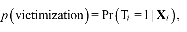
where p(victimization) = propensity of experiencing victimization at Time 2; T_i = 1 (receives treatment) if individual i experienced a victimization at Time 2; and X_i represents the vector of measured Time 1 covariates that predict experiencing a victimization at Time 2.

We calculate propensity scores separately for property victimization and violent victimization. Once propensity scores are calculated, we attempt to match each victim to a non-victim with a similar propensity score using accepted matching procedures. The result is a data set of treatment cases (victim at Time 2) and control cases (non-victim at Time 2) for both property victimization and violent victimization. These cases have been matched on their propensity for treatment (underlying risk of victimization) as measured at Time 1. In the matched data, underlying risk of victimization (i.e., population heterogeneity) has been controlled. If Time 2 victimization significantly increases the likelihood of Time 3 victimization in the matched data set, then state dependence exists net of the effects of population heterogeneity. If there is a significant effect of Time 2 victimization on Time 3 victimization in the unmatched data set, but this effect does not exist in the matched data set, then the effect of victimization on future victimization is spurious, upholding population heterogeneity arguments. There would be evidence of both state dependence and population heterogeneity if victimization at Time 2 predicted victimization at Time 3 in both the matched and unmatched data, but the t statistic associated with Time 2 victimization in the matched data is substantially smaller than the corresponding t statistic in the unmatched data.

We then move to our focal analyses. Here, we examine whether the effects of past victimization on the likelihood of future victimization vary depending upon underlying level of risk. To accomplish this, we stratify the cases in each matched data set by their propensity scores. We then construct a logistic regression model for each stratum, predicting the effects of past victimization on the likelihood of future victimization. We employ the firthlogit procedure in Stata. Firthlogit uses penalized likelihood techniques to correct for errors in the estimation of rare events (Firth, 1993).

Propensity Score Covariates

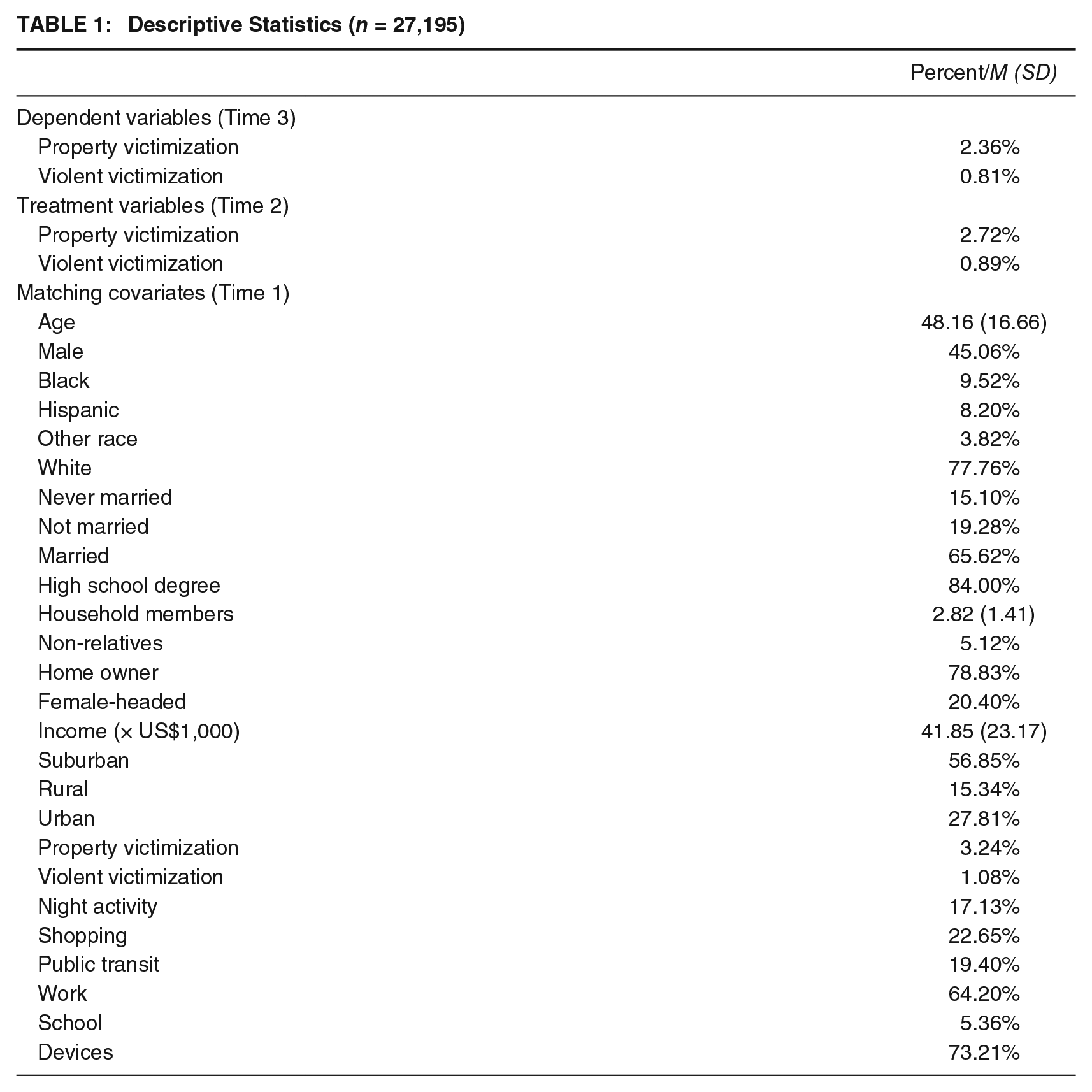
The goal of PSM is to account for individual propensity for selection into the “treatment” group. Here, this means accounting for individual propensity to experience criminal victimization at Time 2. We select as propensity covariates factors that are known to be associated with victimization. As described below, these covariates include demographic characteristics, previous victimization, and routine activities. All covariates are measured at Time 1. See Table 1 for descriptive statistics.

Table 1:

Descriptive Statistics (n = 27,195)

	Percent/M (SD)
Dependent variables (Time 3)
Property victimization	2.36%
Violent victimization	0.81%
Treatment variables (Time 2)
Property victimization	2.72%
Violent victimization	0.89%
Matching covariates (Time 1)
Age	48.16 (16.66)
Male	45.06%
Black	9.52%
Hispanic	8.20%
Other race	3.82%
White	77.76%
Never married	15.10%
Not married	19.28%
Married	65.62%
High school degree	84.00%
Household members	2.82 (1.41)
Non-relatives	5.12%
Home owner	78.83%
Female-headed	20.40%
Income (× US$1,000)	41.85 (23.17)
Suburban	56.85%
Rural	15.34%
Urban	27.81%
Property victimization	3.24%
Violent victimization	1.08%
Night activity	17.13%
Shopping	22.65%
Public transit	19.40%
Work	64.20%
School	5.36%
Devices	73.21%

Demographics

The individual-level demographic measures are age, gender, race, education, and marital status (e.g., Catalano, 2006; Rennison, 2000; Truman, 2011). Age is a known predictor of victimization, with younger persons at increased risk. Age is measured continuously. Because most research finds that men are more likely to experience personal victimization than are women, we include a covariate for Male. Due to the higher victimization risk associated with minority status, we include a set of dummy-coded variables for race (Black, Hispanic, and Other). White is the reference category. On average, non-married persons experience higher rates of victimization than do married persons. Marital status is a set of categorical dummy-coded variables comparing respondents who have never been married (Never Married) and respondents who are separated, widowed, or divorced (Not Married) with respondents who are married. Education is also associated with victimization risk (Tseloni, 2000). Respondents who completed high school are coded “1” for high school degree.

A number of household-level demographic variables affect the likelihood of victimization (e.g., Catalano, 2006; Rennison, 2000; Truman, 2011). Victimization risk increases with household size and with the presence of non-relatives in the home. Household Members is a continuous variable measuring the number of individuals living in the respondent’s household. Non-Relatives is a dichotomous variable measuring whether the respondent lives with any non-relatives. Because income tends to predict neighborhood crime risk, we include reported Household Income as a covariate. We constructed this variable from the 14-category NCVS household income measure, coded each respondent at the midpoint of his or her income interval, and divided this dollar amount by 1,000. The location of one’s home also affects victimization risk. We code urbanicity as a set of categorical dummy-coded variables comparing individuals living in suburban areas (Suburban) and rural areas (Rural) with those living in urban areas.

Time 1 Victimization

It is standard practice to include prior exposure to “treatment” as a matching variable in propensity score models (Apel & Sweeten, 2010). The NCVS utilizes a 6-month window for victimization, which is appropriate here due to the decaying effects of victimization over time (Wittebrood & Nieuwbeerta, 2000). This time frame is also consistent with our measurement of Time 2 and Time 3 victimization. Time 1 Property Victimization is a dichotomous variable measuring whether the respondent reported being a victim of attempted/completed purse snatching, pocket picking, theft of money/goods valued at least US$50, burglary, or motor vehicle theft. Time 1 Violent Victimization measures whether the respondent experienced attempted/completed/threatened aggravated assault, rape, or sexual assault; completed simple assault with injury; or attempted/completed robbery.

Routine Activities

An important predictor of victimization propensity is routine activities. Activities that bring people away from the safety of their homes increase exposure to motivated offenders in situations of reduced guardianship (B. Fisher, Sloan, Cullen, & Lu, 1998; Kennedy & Forde, 1990; Miethe, Stafford, & Long, 1987; Mustaine & Tewksbury, 1998). Risk is heightened further if the activities take place at night or if the activity, itself, makes one an attractive target. We include several lifestyle measures as matching covariates. Our selection of these variables from the NCVS follows previous research (e.g., Averdijk, 2011; Bunch, Clay-Warner, & Lei, 2015; Miethe et al., 1987). Each of these variables is dichotomous and measured at Time 1. Night Activity measures whether the respondent spent the evening away from home almost every night over the past 6 months (Night Activity = 1). Shopping measures whether an individual reported going shopping almost every day over the past 6 months (Shopping = 1). Our coding of these variables follows Tseloni (2000; Tseloni & Pease, 2003), whose analysis of NCVS data found that shopping and night activity affected victimization risk only at these very high levels. In contrast, Tseloni (2000; Tseloni & Pease, 2003) found that any riding of public transit increased victimization risk. Public Transit measures whether the respondent rode public transportation at least once in the last 6 months (Public Transit = 1). Respondents who had a paying job outside of the home within the last week are coded “1” for Work. School measures whether an individual attended school (i.e., high school, college, university, trade school, or vocational school; School = 1). Finally, target-hardening can reduce the risk of victimization (e.g., Averdijk, 2011). Devices is a dichotomous variable measuring whether the individual’s home has devices designed to prevent the entry of an intruder, such as an alarm or a dead bolt.

Treatment Variables

Property Victimization at Time 2 is a dichotomous variable coded “1” if the respondent experienced attempted/completed purse snatching, pocket picking, theft of money/goods valued at least US$50, burglary, or motor vehicle theft in the 6 months prior to Time 2 data collection. Violent Victimization at Time 2 is coded “1” if the respondent experienced attempted/completed/threatened aggravated assault, rape, or sexual assault; completed simple assault with injury; or attempted/completed robbery during the previous 6 months.

Outcome Variables

The outcome variables are Property Victimization at Time 3 and Violent Victimization at Time 3. The coding for these variables is identical to the coding of the treatment variables. The outcome variables are measured at Time 3.

Statistical Analysis

The first step in our analysis is to determine individual propensity for Time 2 victimization for each person in the data set, regardless of whether or not they were actually victimized. Because we analyze property victimization and violent victimization in separate models, we calculated the propensity scores for property and violent victimization separately. An individual’s propensity score was calculated from his or her values on the Time 1 covariates, using the psmatch2 procedure in Stata (v. 11). This procedure uses a probit model to estimate the effects of the covariates on the likelihood of experiencing victimization at Time 2. Each individual’s propensity score is then calculated from his or her values on these covariates. Because the propensity scores represent the probability of experiencing victimization, the possible range for the propensity scores is 0 to 1.

The second step is to create a data set of Time 2 property victims and non-victims matched on their propensity for property victimization at Time 2 and a data set of Time 2 violent crime victims and non-victims matched on their propensity for violent victimization at Time 2. To determine comparability, we use nearest neighbor, one-to-one matching with a caliper of .01. In this approach, a treated case is matched with the closest untreated case whose propensity score is no more than ±.01 from the propensity score of the treated case. The result is two data sets (one for property victimization and one for violent victimization) composed of an equal number of Time 2 victims and non-victims who are equivalent in their propensity for Time 2 victimization. These data sets have removed the effects of population heterogeneity to the extent that the covariates measure the probability of experiencing Time 2 victimization. We then use the firthlogit procedure to estimate the effect of Time 2 victimization on Time 3 victimization.

Next, we examine whether the effects of a victimization event on subsequent victimization risk varies depending upon one’s underlying propensity for victimization. To test for these differential vulnerability effects, we stratify the matched sample into quartiles based upon propensity scores and examine the effects of Time 2 victimization on Time 3 victimization within each group (see A. S. Jones, D’Agostino, Gondolf, & Heckert, 2004; King, Massoglia, & MacMillan, 2007). Variation in the effects of Time 2 victimization on Time 3 victimization across quartiles would indicate differential vulnerability to the experience of victimization.

Results

Property Victimization

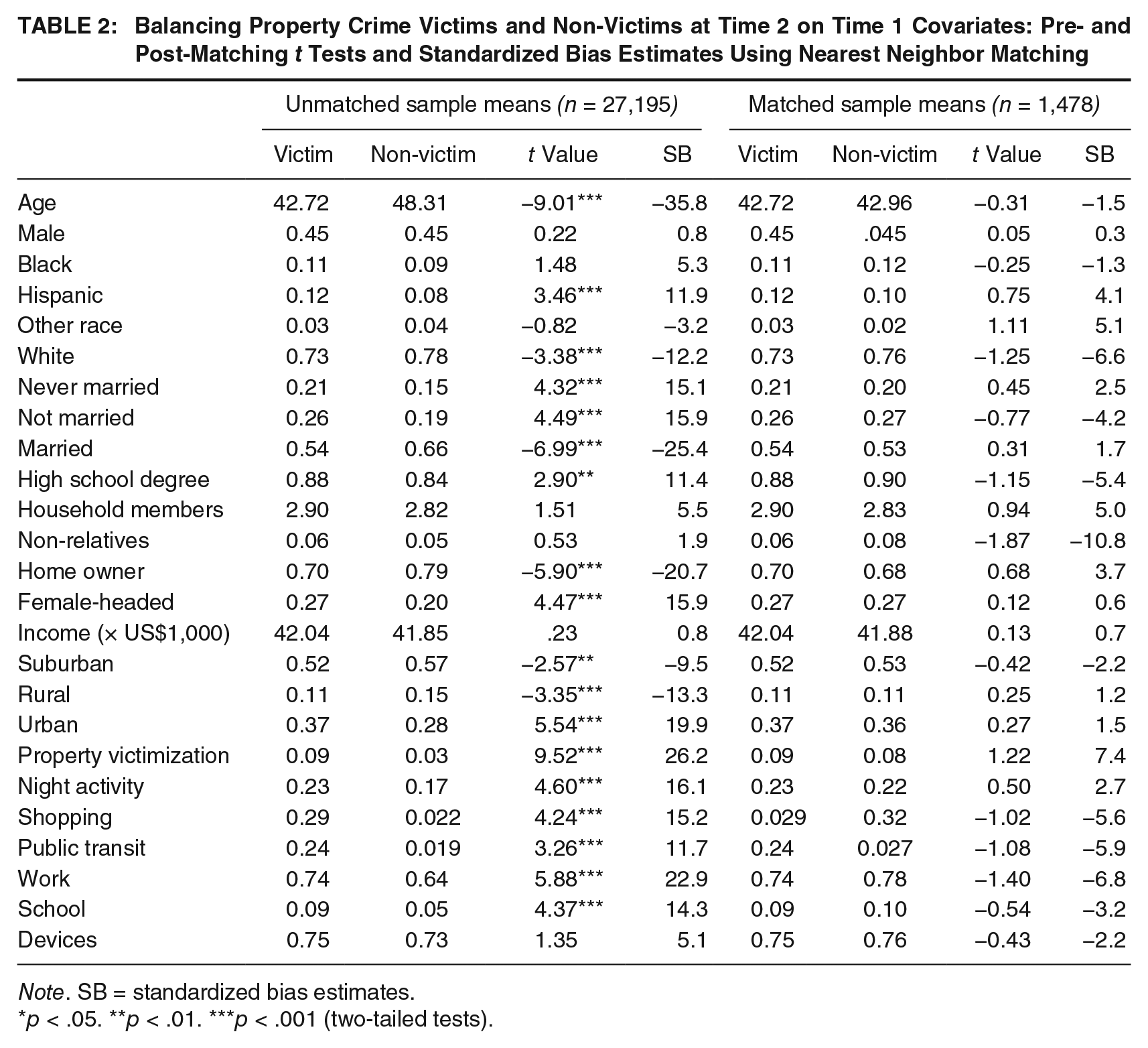
In the full sample, there are significant differences between Time 2 property crime victims and non-victims on a number of factors known to be associated with victimization risk (see Table 2). Victims were younger than non-victims and more likely to be high school graduates. Married individuals were less likely to experience property victimization than were non-married or never-married individuals, as were those who lived in rural or suburban areas. Whites were less likely to experience property victimization than were non-Whites, and Hispanics experienced an elevated risk. Victims were more likely to live in female-headed households and in dwellings that were not owner-occupied. There were also significant differences on all of the routine activity variables. In each case, Time 2 victims indicated a higher level of participation in these activities at Time 1 than did those who were not victimized at Time 2. Finally, those who experienced property victimization in the focal time period (Time 2) were significantly more likely to have experienced victimization in the previous time period than were non-victims.

Table 2:

Balancing Property Crime Victims and Non-Victims at Time 2 on Time 1 Covariates: Pre- and Post-Matching t Tests and Standardized Bias Estimates Using Nearest Neighbor Matching

	Unmatched sample means (n = 27,195)				Matched sample means (n = 1,478)
	Victim	Non-victim	t Value	SB	Victim	Non-victim	t Value	SB
Age	42.72	48.31	−9.01***	−35.8	42.72	42.96	−0.31	−1.5
Male	0.45	0.45	0.22	0.8	0.45	.045	0.05	0.3
Black	0.11	0.09	1.48	5.3	0.11	0.12	−0.25	−1.3
Hispanic	0.12	0.08	3.46***	11.9	0.12	0.10	0.75	4.1
Other race	0.03	0.04	−0.82	−3.2	0.03	0.02	1.11	5.1
White	0.73	0.78	−3.38***	−12.2	0.73	0.76	−1.25	−6.6
Never married	0.21	0.15	4.32***	15.1	0.21	0.20	0.45	2.5
Not married	0.26	0.19	4.49***	15.9	0.26	0.27	−0.77	−4.2
Married	0.54	0.66	−6.99***	−25.4	0.54	0.53	0.31	1.7
High school degree	0.88	0.84	2.90**	11.4	0.88	0.90	−1.15	−5.4
Household members	2.90	2.82	1.51	5.5	2.90	2.83	0.94	5.0
Non-relatives	0.06	0.05	0.53	1.9	0.06	0.08	−1.87	−10.8
Home owner	0.70	0.79	−5.90***	−20.7	0.70	0.68	0.68	3.7
Female-headed	0.27	0.20	4.47***	15.9	0.27	0.27	0.12	0.6
Income (× US$1,000)	42.04	41.85	.23	0.8	42.04	41.88	0.13	0.7
Suburban	0.52	0.57	−2.57**	−9.5	0.52	0.53	−0.42	−2.2
Rural	0.11	0.15	−3.35***	−13.3	0.11	0.11	0.25	1.2
Urban	0.37	0.28	5.54***	19.9	0.37	0.36	0.27	1.5
Property victimization	0.09	0.03	9.52***	26.2	0.09	0.08	1.22	7.4
Night activity	0.23	0.17	4.60***	16.1	0.23	0.22	0.50	2.7
Shopping	0.29	0.022	4.24***	15.2	0.029	0.32	−1.02	−5.6
Public transit	0.24	0.019	3.26***	11.7	0.24	0.027	−1.08	−5.9
Work	0.74	0.64	5.88***	22.9	0.74	0.78	−1.40	−6.8
School	0.09	0.05	4.37***	14.3	0.09	0.10	−0.54	−3.2
Devices	0.75	0.73	1.35	5.1	0.75	0.76	−0.43	−2.2

Note. SB = standardized bias estimates.

p < .05. **p < .01. ***p < .001 (two-tailed tests).

Matching

We identified matches for all 739 individuals in the sample who experienced property victimization at Time 2 (treatment cases). This resulted in a data set of 739 victims and 739 non-victims, matched on their propensity for victimization at Time 2. To verify that our matching procedure successfully balanced on all potentially confounding Time 1 covariates, we compared the means for victims and non-victims in the matched sample on each of the propensity variables. As seen in Table 2, there are no significant differences between victims and non-victims in the matched sample.

We also examined the standardized bias estimates (SB), which provide an additional method for assessing balance. The SB of a covariate is the mean difference between treated and untreated cases as a percentage of the average standard deviation (Rosenbaum & Rubin, 1985). If a given covariate has an SB value of 20 or above, then that covariate is not adequately balanced across groups in the matched data (Rosenbaum & Rubin, 1985). Table 2 shows that the covariates in the matched sample all have SB well below this threshold. Thus, the SB values provide additional evidence of a successful match.

Findings

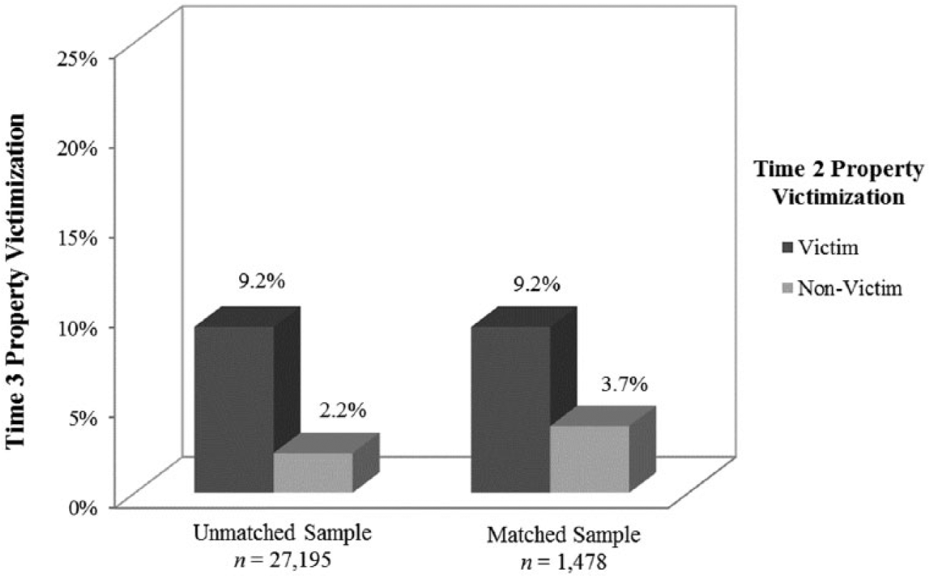
Consistent with previous research, we find that both state dependence and heterogeneity processes contribute to risk of repeat property victimization (see Figure 1). Property victimization at Time 2 is significantly associated with odds of Time 3 property victimization in the unmatched sample (t = 12.44, p < .001). Time 2 victimization also predicts Time 3 victimization in the matched data (t = 4.37, p < .001) though the effect is smaller. As reflected in Figure 1, 9.2% of Time 2 property crime victims were victimized in Time 3. In the unmatched data, which contains all survey respondents, only 2.2% of those who were not victimized at Time 2 experienced later property victimization. However in the matched data, 3.7% of Time 2 non-victims experienced Time 3 victimization. The increase in the proportion of Time 3 victims in the matched data indicates that population heterogeneity does account for some of the association between Time 2 and Time 3 victimization. Nonetheless, the significant t statistic and substantial difference in the proportion of Time 2 victims and non-victims experiencing victimization at Time 3 in the matched data set (9% vs. 3.7%) provide clear evidence of positive state dependence.

Figure 1:

Property Crime: Effects of Time 2 Victimization on Time 3 Victimization

Analysis of the matched data stratified by underlying propensity for victimization, however, reveals that positive state dependence effects exist only for individuals in the three lowest quartiles (see Figure 2). For those in the lowest risk group, Time 2 property victimization is significantly related to Time 3 property victimization (p < .05, propensity score range = .006-.022, odds ratio [OR] = 3.4). Results are similar in the two middle quartiles. Time 2 property victimization significantly predicts Time 3 property victimization for those with medium-low propensity for victimization (p < .05, propensity score range = .023-.033, OR = 2.67) and for those with medium-high victimization propensity (p < .01, propensity score range = .034-.052, OR = 3.45). The ORs indicate that experiencing property victimization at Time 2 boosts the risk of Time 3 property victimization by approximately 200% for those in the lower three quartiles. In contrast, not only is there no significant state dependence effect in the highest risk group, but also the direction of effects is opposite to that found in the other quartiles (p > .1, propensity score range = .052-.187).

Figure 2:

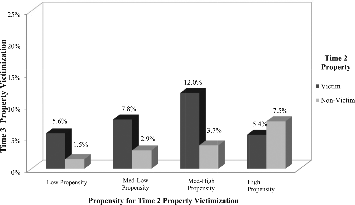
Property Crime: Effects of Time 2 Victimization on Time 3 Victimization by Propensity for Victimization (n = 1,478)

Violent Victimization

Violent crime victims and non-victims differed on a number of dimensions in the unmatched data (see Table 3). Victims of violent crime at Time 2 were disproportionately young, unmarried, and male. They were also more likely to live in non-owner occupied housing, with non-relatives, and in urban areas. All of the routine activity variables except for shopping differentiated between Time 2 violent crime victims and non-victims. Unlike in property victimization, however, Hispanic persons experienced less violent victimization than did non-Hispanics, whereas Whites had higher rates than non-Whites.

Table 3:

Balancing Violent Crime Victims and Non-Victims at Time 2 on Time 1 Covariates: Pre- and Post-Matching t Tests and Standardized Bias Estimates Using Nearest Neighbor Matching

	Unmatched sample means (n = 27,195)				Matched sample means (n = 482)
	Victim	Non-victim	t Value	SB	Victim	Non-victim	t Value	SB
Age	39.52	48.24	−8.11***	−59.6	39.60	38.54	0.88	7.2
Male	0.54	0.45	2.85**	18.4	0.54	0.59	−1.19	−10.8
Black	0.08	0.10	−0.67	−4.4	0.08	0.10	−0.78	−7.3
Hispanic	0.03	0.08	−2.79**	−21.3	0.03	0.04	−0.48	−3.6
Other race	0.03	0.04	−0.42	−2.8	0.03	0.02	0.54	4.5
White	0.84	0.78	2.30*	15.7	0.84	0.82	0.48	4.2
Never married	0.28	0.15	5.68***	32.3	0.28	0.29	−0.30	−3.1
Not married	0.22	0.19	1.04	6.5	0.22	0.18	1.14	10.3
Married	0.50	0.66	−5.14***	−32.3	0.50	0.53	−0.64	−6.0
High school degree	0.86	0.84	0.84	5.6	0.86	0.84	0.63	5.8
Household members	2.78	2.82	−0.49	−3.1	2.78	2.87	−0.70	−6.3
Non-relatives	0.10	0.05	3.11**	17.0	0.10	0.09	0.16	1.6
Home owner	0.66	0.79	−4.87***	−29.0	0.66	0.70	−0.98	−9.4
Female-headed	0.25	0.20	1.87	11.6	0.25	0.22	0.64	5.9
Income (× US$1,000)	38.94	41.88	−1.97*	−12.8	39.00	40.39	−0.66	−6.1
Suburban	0.45	0.57	−3.59***	−23.1	0.46	0.47	−0.36	−3.3
Rural	0.10	0.15	−2.17*	−15.1	0.10	0.10	0.00	0.0
Urban	0.44	0.28	5.72***	35.0	0.44	0.42	0.37	3.5
Violent victimization	0.10	0.01	12.77***	38.7	0.09	0.10	−0.16	−1.9
Night activity	0.26	0.17	3.69***	22.0	0.26	0.26	0.00	0.0
Shopping	0.23	0.23	0.03	0.2	0.23	0.26	−0.74	−6.9
Public transit	0.26	0.19	2.62**	16.0	0.26	0.24	0.31	3.0
Work	0.74	0.64	3.05**	20.5	0.73	0.79	−1.50	−12.6
School	0.09	0.05	2.59**	14.6	0.09	0.08	0.49	4.8
Devices	0.75	0.73	0.56	3.6	0.75	0.81	−1.54	−13.2

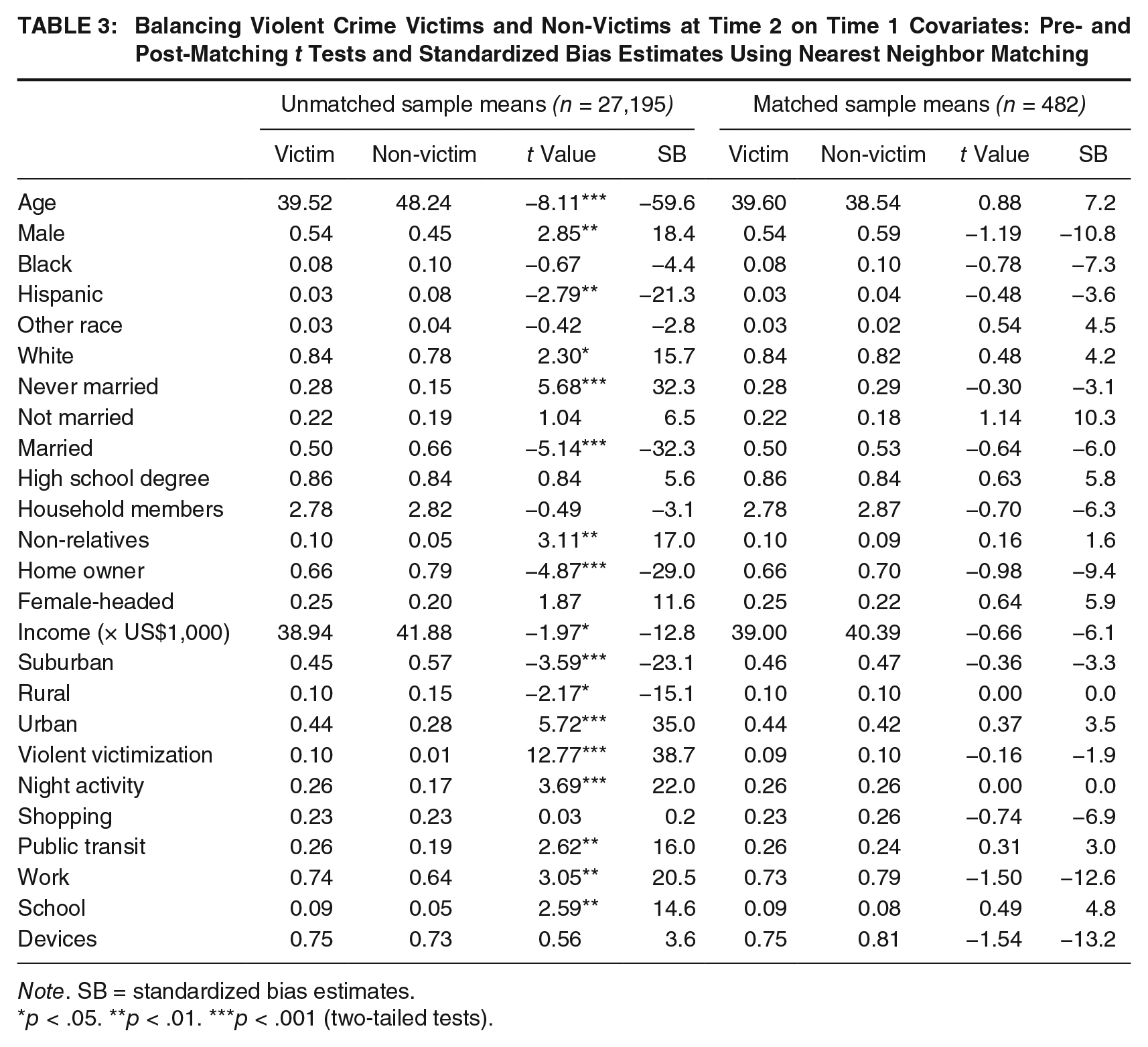
Note. SB = standardized bias estimates.

p < .05. **p < .01. ***p < .001 (two-tailed tests).

Matching

We identified matches for 241 of the 242 individuals in the sample who experienced violent victimization at Time 2 (treatment cases). This resulted in a data set of 241victims and 241 non-victims, matched on their propensity for violent victimization at Time 2. A comparison of the means reveals that there are no significant differences between victims and non-victims in the matched sample (see Table 2). Likewise, the SB are all well below 20, indicating a successful match.²

Findings

We find that Time 2 violent victimization is significantly associated with Time 3 violent victimization in the full unmatched sample (t = 19.58, p < .001). In the matched data, which controls for heterogeneity in underlying propensity for violent victimization, Time 2 violent victimization continues to predict Time 3 victimization (t = 4.10, p < .001). As shown in Figure 3, however, there is a reduction in the treatment effect once population heterogeneity is controlled. Twelve percent of Time 2 violent crime victims were victimized at Time 3. In the unmatched sample, only 0.7% of those who were not victimized at Time 2 experienced later violent victimization, while in the matched data, 2.5% of Time 2 non-victims were victimized at Time 3. Nonetheless, the gap between the proportion of Time 2 victims and non-victims who were victimized at Time 3 in the matched data is substantial (12% vs. 2.5%), and the t statistic is significant (t = 4.10), indicating that strong state dependence effects remain.

Figure 3:

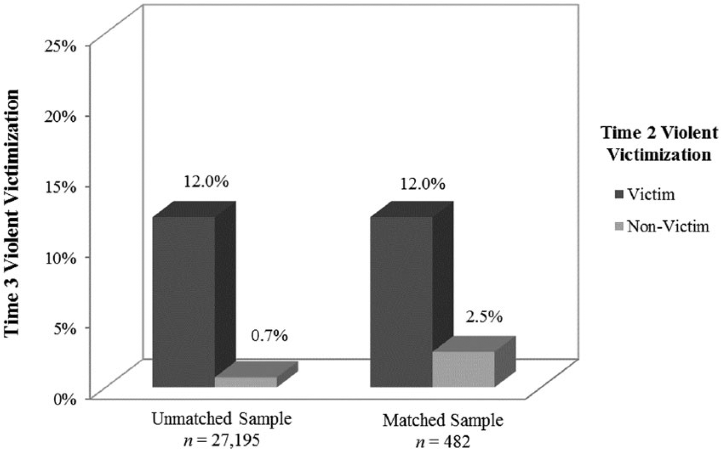
Violent Crime: Effects of Time 2 Victimization on Time 3 Victimization

State dependence effects for violent victimization, however, are not uniform across levels of victimization propensity (see Figure 4). Individuals in the first quartile, representing the highest level of underlying risk for violent victimization at Time 2, had propensity scores ranging from .024 to .171. Time 2 victimization had a significant effect on Time 3 victimization for persons in this high-risk group (p < .05, OR = 3.91). For these individuals, experiencing a violent victimization at Time 2 increased odds of violent victimization at Time 3 by almost 300%. However, there was no significant effect of Time 2 victimization on Time 3 victimization in the medium-high propensity group (p = .06, propensity score range = .013-.023), the medium-low propensity group (p = .18, propensity score range = .008-.013), or the low propensity group (p = .29, propensity score range = .00-.007). This pattern of effects indicates that experiencing a violent victimization only increased risk of subsequent victimization for those with the highest level of underlying victimization propensity. There is no evidence of state dependence among those with medium and low levels of risk.

Figure 4:

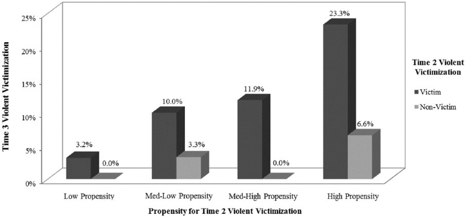
Violent Crime: Effects of Time 2 Victimization on Time 3 Victimization by Propensity for Victimization (n = 482)

It is possible that our inability to detect significant effects in certain quartiles for violent victimization is due to small sample size. To consider this possibility, we divided the violent victimization data set into thirds by propensity scores, thereby increasing the sample size of each strata to approximately 160 cases. We again run firthlogit models. Results were consistent with the quartile analysis. There was a statistically significant state dependence effect only for those in the highest victimization propensity group (p < .01, OR = 5.4). There was no significant effect of Time 2 violent victimization on Time 3 violent victimization for those with either medium-levels of victimization propensity (p = .1) or those with low levels of victimization propensity (p = .24).

Summary

Results indicate that state dependence effects are not consistent across levels of underlying risk and that patterns of state dependence differ for property and violent victimization. There is no evidence of state dependence effects for property crime among those with high propensity for victimization. Positive state dependence effects exist, however, for those with medium and low propensity for property victimization. There is an opposite pattern of effects for violent victimization. There is a statistically significant state dependence effect for those with high levels of underlying victimization propensity and no evidence of state dependence for those at medium and low levels of propensity for violent victimization.

Discussion

In documenting variability in state dependence effects, we offer support for a more nuanced interpretation of the mixed model of repeat victimization. Consistent with previous research, we find that while population heterogeneity accounts for some portion of repeat victimization risk, state dependence effects remain after controlling for population heterogeneity (e.g., Lauritsen & Davis Quinet, 1995; Ousey et al., 2008; Wittebrood & Nieuwbeerta, 2000). Moving beyond previous research, however, we find that state dependence effects are not consistent across varying levels of underlying risk. The pattern of effects also differ for violent and property victimization.

The pattern of effects for repeat property victimization supports the victimization salience argument. This means that property victimization has the greatest impact on those least likely to experience it. Persons in the high propensity group may have simply hit a statistical ceiling on risk, as their high levels of underlying propensity are so great that there is little that a single event can do to increase the odds of future victimization. It is also possible that victim labeling, which occurs when an offender selects a target as a result of information gained about that individual or his or her property during the course of a previous victimization, contributes to this effect. For example, researchers posit that learning how to enter and exit a home undetected during the course of an initial burglary facilitates completion of a subsequent burglary of the same location (e.g., Sparks, 1981; Johnson et al., 2009). Persons with low individual propensity for burglary victimization tend to live in communities with similar low risk neighbors (i.e., those with effective guardianship), giving offenders a particularly strong incentive to burglarize the home again as nearby houses would be considerably more difficult to access. This would be less important when most houses are unguarded, however, as the reduced guardianship makes many other homes in the community attractive targets. Similar arguments would apply to other property crimes where guardianship is an issue, such as theft of items in a motor vehicle. The logic of this argument is less applicable to violent crime, which may explain why victimization salience was evident only for property victimization.

In contrast, the pattern of effects for violent victimization suggests support for the compounding vulnerabilities argument as only those with high levels of underlying propensity for violent victimization experienced a boost in risk from a victimization event. These results indicate that the same factors that predispose individuals to violent victimization also amplify the effects of a victimization event on odds of future victimization. One possible mediating factor is the display of PTSD symptoms. Persons with characteristics that make them more susceptible to victimization (e.g., youth, minority status, and low socio-economic status) are also more likely to experience symptoms of PTSD following a traumatic event (Brewin et al., 2000). Symptoms of PTSD reduce one’s ability to respond effectively to threat, thereby increasing risk of subsequent victimization (Cougle et al., 2009; Kunst & Winkel, 2013). The lower incidence of PTSD following property crime and the fact that mounting an effective response to threat is primarily relevant to violent victimization may partly explain why the compounding vulnerabilities argument does not apply to repeat property victimization. In addition, those who are at risk of experiencing violent crime are also more likely to retaliate, which can lead to revictimization (Jacobs & Wright, 2006).

Our findings have a number of implications for understanding repeat victimization. First, because individuals are differentially susceptible to state dependence effects, theories of repeat victimization must account not only for underlying vulnerabilities in victimization risk, but also for susceptibility to the “boosting” effect of victimization on future victimization risk. This suggests a shift in the way that researchers approach the study of repeat victimization: Instead of asking “whether” there is a state dependence effect, researchers should ask “for whom” is there a state dependence effect. Here we have focused on overall propensity for victimization, but future theoretical and empirical work could consider whether certain predisposing factors increase susceptibility to state dependence effects more than do others.

Second, differential patterns of state dependence in violent and property victimization indicate that the dynamics of repeat victimization vary across crime type. Because research on repeat victimization typically focuses on a single crime category, there is little theoretical literature discussing how the experience of violent and property victimization may differentially affect repeat victimization risk (Tillyer, 2014). In examining overlap in victimization experiences, Schreck, Ousey, Fisher, and Wilcox (2012), however, acknowledged potential differences in the experience of violent and non-violent victimization. They found that though there was considerable overlap in violent and non-violent victimization over time, a substantial proportion of victims were more likely to experience violent than non-violent victimization, and that this pattern of victimization experiences could be predicted. Complementing their findings, our research indicates that victimization propensity shapes the experience of violent and property victimization in different ways, leading to variation in repeat victimization risk.

Limitations And Directions For Future Research

Our research, of course, is not without limitations. For example, our inability to include as covariates some individual-level factors known to affect victimization risk could introduce bias into the model. In particular, the NCVS does not contain measures of offending. It is well established that offending and victimization are associated, though the direction of these effects is not well established (see Ousey, Wilcox, & Fisher, 2011). We were, however, able to include as covariates many of the factors that predict offending, such as age, sex, household income, marital status, and education. In doing so, we likely account for some of the influence that offending may have on underlying risk of victimization. Similarly, the NCVS does not include measures of self-control, which is associated with criminal victimization (Pratt, Turanovic, Fox, & Wright, 2014; Schreck, 1999). Recent research, however, finds that self-control varies across time (Burt, Simons, & Simons, 2008) and that it is affected by victimization (Agnew et al., 2011; Ousey et al., 2008). This suggests that self-control may not be a stable source of difference between victims and non-victims. Nonetheless, if self-control and offending are causally related to repeat victimization and the variance associated with these factors is not accounted for by other variables, then our propensity score models will not fully control for risk heterogeneity. As a result, the findings that we attribute to state dependence could be confounded with underlying differences in self-control and/or offending between Time 2 victims and non-victims. For this reason, we recognize that future research should consider the roles that both offending and self-control play in victimization propensity and repeat victimization.

Another limitation is the age of the data. We used data from the 1998-1999 NCVS because these are the most recent years of the survey that included measures of routine activities. Because findings may not be generalizable across time, it is important to verify findings with newer data. It would be particularly important to test predictions with data that include information about both online and traditional forms of victimization, given the increasingly important role that Internet use plays in victimization risk (L. M. Jones, Mitchell, & Finkelhor, 2012; Reisig, Pratt, & Holtfreter, 2009). As we are examining underlying social processes, however, we would expect that our basic findings would hold despite the fact that the specific factors that indicate risk exposure and the specific crimes committed may change across time.

Despite these data limitations, the overall strengths of the NCVS outweigh its weaknesses. The NCVS is currently the best nationally representative, longitudinal data set on victimization in the United States. Also, while most victimization surveys focus exclusively on adolescents, the NCVS includes adults. As a result, we are able to generalize our findings across a much larger population than is possible with studies using non-representative or more limited samples (e.g., Lauritsen & Davis Quinet, 1995; Ousey et al., 2011; Schreck et al., 2006; Wilcox et al., 2006). Finally, the 6-month lag between interviews in the NCVS provides an appropriate time frame for our longitudinal analysis. Studies with longer periods between interviews risk respondent recall errors, while shorter time periods are less likely to capture a full-range of victimization experiences.

While our study provides a more nuanced analysis of the joint effects of state dependence and heterogeneity processes than has previous research, we did not attempt to identify the specific mechanisms through which state dependence processes operate. Existing research suggests several potential mechanisms, though there is little consensus. In their study of adolescents, Schreck et al. (2006) reported that the effects of violent victimization on future violent victimization were mediated by risky behavior, as measured by association with delinquent peers. In contrast, Averdijk (2011) found that violent victimization did not increase participation in risky routine activities (see also Bunch, Clay-Warner, & McMahon-Howard, 2014). Offender behavior may also link victimization events. Offenders gain information about a person or a location in the course of committing a crime and then are able to use this information to increase success of subsequent victimization of this individual or place. Recent spatial analyses of property victimization patterns indicate support for this argument (e.g., Johnson et al., 2009). As suggested by this research and by our finding that state dependence patterns differed for violent and property crime, future research should consider how mechanisms for repeat victimization may differ by type of crime.

Conclusion

While research has suggested that both state dependence and population heterogeneity play some role in repeat victimization, much of the debate has focused on the relative importance of each process; yet, the exact nature of the relationship has remained unclear. Here, we find that individuals experience differential vulnerability to state dependence effects based upon their underlying risk for victimization, and this relationship differs for property crime and violent crime. For property crime, we find evidence of victimization salience: Property victimization caused the greatest “boost” in victimization risk among those who were unlikely to be victims. In contrast, the results for violent victimization suggested a pattern of compounding vulnerabilities in which state dependence effects existed only for those with the highest underlying risk of violent victimization. Recognition of these patterns increases our understanding of repeat victimization and suggests new directions for research.

Footnotes

Data used in this article were obtained from the International Consortium for Political and Social Research (ICPSR).

Notes

Jody Clay-Warner is Meigs distinguished professor of sociology and department head at the University of Georgia. Her research examines sexual violence, causes and consequences of criminal victimization, and fear of crime.

Jackson M. Bunch is an assistant professor of sociology at the University of Montana. His research examines the causes and consequences of criminal victimization, including routine activities, fear of crime, and the relationship between offending and victimization.

Jennifer McMahon-Howard is an associate professor in the Department of Sociology and Criminal Justice at Kennesaw State University. Her current research focuses on criminal victimization, sexual violence, human trafficking, and legal change.

References

Agnew

(1992). Foundation for a general strain theory of crime and delinquency. Criminology, 30, 47-88.

Agnew

(2006). Pressured into crime: An overview of general strain theory. Los Angeles, CA: Roxbury.

Agnew

Scheuerman

Grosholz

Isom

Watson

Thaxton

(2011). Does victimization reduce self-control? A longitudinal analysis. Journal of Criminal Justice, 39, 169-174.

American Psychiatric Association. (2013). Diagnostic and statistical manual of mental disorders (5th ed.). Arlington, VA: American Psychiatric Publishing.

Apel

R. J.

Sweeten

(2010). Propensity score matching in criminology and criminal justice. In Piquero

A. R.

Weisburd

(Eds.), Handbook of quantitative criminology (pp. 543-562). New York, NY: Springer.

Atkeson

B. M.

Calhoun

K. S.

Resick

P. A.

Ellis

E. M.

(1982). Victims of rape: Repeated assessment of depressive symptoms. Journal of Consulting and Clinical Psychology, 50, 96-102.

Averdijk

(2011). Reciprocal effects of victimization and routine activities. Journal of Quantitative Criminology, 27, 125-149.

Averdijk

Loeber

(2012). The role of self-control in the link between prior and future victimization: An indirect test. International Review of Victimology, 18, 189-206.

Becker

S. O.

Ichino

(2002). Estimation of average treatment effects based on propensity scores. The Stata Journal, 2, 358-377.

10.

Bernasco

(2008). Them again? Same-offender involvement in repeat and near repeat burglaries. European Journal of Criminology, 5, 411-431.

11.

Brewin

C. R.

Andrews

Valentine

J. D.

(2000). Meta-analysis of risk factors for posttraumatic stress disorder in trauma-exposed adults. Journal of Consulting and Clinical Psychology, 68, 748-766.

12.

Bunch

Clay-Warner

Lei

M.-K.

(2015). Demographic characteristics and victimization risk: Testing the mediating effects of routine activities. Crime & Delinquency, 61, 1181-1205.

13.

Bunch

Clay-Warner

McMahon-Howard

(2014). The effects of victimization on routine activities. Criminal Justice & Behavior, 41, 575-593.

14.

Bureau of Justice Statistics. (1999). National Crime Victimization Survey, 1992-1999: Codebook for the 1992-1994 full files. Ann Arbor: Inter-University Consortium for Political and Social Research, University of Michigan.

15.

Bureau of Justice Statistics. (2014). National Crime Victimization Survey technical document (NCJ Publication No. 247252). Washington, DC: U.S. Government Printing Office.

16.

Burt

C. H.

Simons

R. L.

Simons

L. G.

(2008). A longitudinal test of the effects of parenting and the stability of self-control: Negative evidence for the general theory of crime. Criminology, 44, 353-396.

17.

Catalano

S. M.

(2006). Criminal victimization, 2005. Washington, DC: Bureau of Justice Statistics, U.S. Department of Justice.

18.

Cohen

Felson

(1979). Social change and crime rate trends: A routine activity approach. American Sociological Review, 44, 588-608.

19.

Cook

P. J.

(1986). The demand and supply of criminal opportunities. Crime and Justice, Annual Review of Research, 7, 1-27.

20.

Cougle

J. R.

Resnick

Kilpatrick

D. G.

(2009). A prospective examination of PTSD symptoms as risk factors for subsequent exposure to potentially traumatic events among women. Journal of Abnormal Psychology, 118, 405-411.

21.

Davis

R. C.

Taylor

Lurigio

A. J.

(1996). Adjusting to criminal victimization: The correlates of postcrime distress. Violence and Victims, 11, 21-38.

22.

Dugan

(1999). The effect of criminal victimization on a household’s moving decision. Criminology, 37, 903-930.

23.

Farrell

Pease

(1993). Once bitten, twice bitten: Repeat victimization and its implications for crime prevention (Police Research Group, Crime Prevention Unit, Paper No. 46). London, England: Home Office Police Department.

24.

Farrell

Phillips

Pease

(1995). Like taking candy: Why does repeat victimization occur? British Journal of Criminology, 35, 384-399.

25.

Farrington

D. P.

(1993). Understanding and preventing bullying. Crime and Justice, 17, 381-458.

26.

Firth

(1993). Bias reduction of maximum likelihood estimates. Biometrika, 80, 27-38.

27.

Fisher

Sloan

Cullen

(1998). Crime in the ivory tower: The level and sources of student victimization. Criminology, 36, 671-710.

28.

Fisher

R. A.

(1935). The design of experiments. New York, NY: Hafner Publishing.

29.

Foster

E. M.

(2003). Propensity score matching: An illustrative analysis of dose response. Medical Care, 41, 1183-1192.

30.

Friedman

Biscoff

Davis

Person

(1982). Victims and helpers: Reactions to crime (Grant Report No. 79-NIAX0059). Washington, DC: National Institute of Justice.

31.

Hindelang

Gottfredson

Garofalo

(1978). Victims of personal crime: An empirical foundation for a theory of personal victimization. Cambridge, MA: Ballinger.

32.

Jacobs

B. A.

Wright

(2006). Street justice: Retaliation in the criminal underworld. Cambridge, UK: Cambridge University Press.

33.

Johnson

S. D.

Summers

Pease

(2009). Offender as forager? A direct test of the boost account of victimization. Journal of Quantitative Criminology, 25, 181-200.

34.

Jones

A. S.

D’Agostino

R. B.

Jr. Gondolf

E. W.

Heckert

(2004). Assessing the effect of batterer program completion on reassault using propensity scores. Journal of Interpersonal Violence, 19, 1002-1020.

35.

Jones

L. M.

Mitchell

K. J.

Finkelhor

(2012). Trends in youth internet victimization: Findings from three youth internet safety surveys 2000–2010. Journal of Adolescent Health, 50, 179-186.

36.

Kahneman

Tversky

(1979). Prospect theory: An analysis of decision under risk. Econometrica: Journal of the Econometric Society, 47, 263-291.

37.

Kennedy

Forde

(1990). Routine activities and crime: An analysis of victimization in Canada. Criminology, 28, 137-152.

38.

King

R. D.

Massoglia

MacMillan

(2007). The context of marriage and crime: Gender, the propensity to marry, and offending in early adulthood. Criminology, 45, 33-65.

39.

Kunst

M. J.

Winkel

F. W.

(2013). Exploring the impact of dysfunctional posttraumatic survival responses on crime revictimization. Violence and Victims, 28, 670-680.

40.

Lauritsen

J. L.

Davis Quinet

(1995). Repeat victimization among adolescents and young adults. Journal of Quantitative Criminology, 11, 143-166.

41.

Lurigio

A. J.

(1987). Are all victims alike? The adverse, generalized, and differential impact of crime. Crime & Delinquency, 33, 452-467.

42.

Lynch

J. P.

Pridemore

(2011). Crime in international perspective. In Wilson

J. Q.

Petersilia

(Eds.), Crime and public policy (pp. 5-52). New York, NY: Oxford University Press.

43.

Maguire

Corbett

(1987). The effects of crime and the work of victims support schemes. Aldershot, Ontario, Canada: Gower.

44.

Miethe

Stafford

Long

J. S.

(1987). Social differentiation in criminal victimization: A test of routine activities/lifestyle theories. American Sociological Review, 52, 184-194.

45.

Mustaine

Tewksbury

(1998). Predicting risks of larceny theft victimization: A routine activities analysis using refined lifestyle measures. Criminology, 36, 829-858.

46.

Ousey

G. C.

Wilcox

Brummel

(2008). Déjà vu all over again: Investigating temporal continuity of adolescent victimization. Journal of Quantitative Criminology, 24, 307-335.

47.

Ousey

G. C.

Wilcox

Fisher

B. S.

(2011). Something old, something new: Revisiting competing hypotheses of the victimization-offending relationship among adolescents. Journal of Quantitative Criminology, 27, 53-84.

48.

Pease

(1998). Repeat victimization: Taking stock (Crime Detection and Prevention Series Paper 90). London, England: Home Office.

49.

Pratt

T. C.

Turanovic

J. J.

Fox

K. A.

Wright

K. A.

(2014). Self-control and victimization: A meta-analysis. Criminology, 52, 87-116.

50.

Reid

J. A.

Sullivan

C. J.

(2009). A latent class typology of juvenile victims and exploration of risk factors and outcomes of victimization. Criminal Justice and Behavior, 36, 1001-1024.

51.

Reisig

M. D.

Pratt

T. C.

Holtfreter

(2009). Perceived risk of internet theft victimization: Examining the effects of social vulnerability and financial impulsivity. Criminal Justice and Behavior, 36, 369-384.

52.

Rennison

C. M.

(2000). Criminal victimization, 1999. Washington, DC: Bureau of Justice Statistics, U.S. Department of Justice.

53.

Rosenbaum

P. R.

Rubin

(1983). The central role of the propensity score in observational studies for causal effects. Biometrika, 70, 41-55.

54.

Rosenbaum

P. R.

Rubin

(1985). Constructing a control group using multivariate matched sampling methods that incorporate the propensity score. The American Statistician, 39, 33-38.

55.

Rountree

Land

(1996). Burglary victimization, perceptions of crime risk, and routine activities: A multilevel analysis across Seattle neighborhoods and census tracts. Journal of Research in Crime & Delinquency, 33, 147-180.

56.

Schreck

C. J.

(1999). Criminal victimization and low self-control: An extension and test of a general theory of crime. Justice Quarterly, 16, 633-654.

57.

Schreck

C. J.

Ousey

G. C.

Fisher

B. S.

Wilcox

(2012). Examining what makes violent crime victims unique: Extending statistical methods for studying specialization to the analysis of crime victims. Journal of Quantitative Criminology, 28, 651-671.

58.

Schreck

C. J.

Stewart

Fisher

B. S.

(2006). Self-control, victimization, and their influence on risky lifestyles: A longitudinal analysis using panel data. Journal of Quantitative Criminology, 22, 319-340.

59.

Schwartz

Pitts

(1995). Exploring a feminist routine activities approach to explaining sexual assault. Justice Quarterly, 12, 9-31.

60.

Skogan

W. G.

Maxfield

(1981). Coping with crime. Beverly Hills, CA: SAGE.

61.

Sparks

R. F.

(1981). Multiple victimization: Evidence, theory, and future research. The Journal of Criminal Law and Criminology, 72, 762-778.

62.

Spitzer

R. L.

Kroenke

Williams

J. B.

Löwe

(2006). A brief measure for assessing generalized anxiety disorder: The GAD-7. Archives of Internal Medicine, 166, 1092-1097.

63.

Sullivan

C. J.

Wilcox

Ousey

G. C.

(2011). Trajectories of victimization from early to mid-adolescence. Criminal Justice and Behavior, 38, 85-104.

64.

Tillyer

M. S.

(2014). Violent victimization across the life course: Moving a “victim careers” agenda forward. Criminal Justice and Behavior, 41, 593-612.

65.

Truman

J. L.

(2011). Criminal victimization, 2010. Washington, DC: Bureau of Justice Statistics, U.S. Department of Justice.

66.

Tseloni

(2000). Personal criminal victimization in the United States: Fixed and random effects of individual and household characteristics. Journal of Quantitative Criminology, 16, 415-442.

67.

Tseloni

Pease

(2003). Repeat personal victimization: “Boosts” or “flags”? British Journal of Criminology, 43, 196-212.

68.

Tseloni

Pease

(2004). Repeat personal victimization: Random effects, event dependence and unexplained heterogeneity. British Journal of Criminology, 44, 931-945.

69.

Turanovic

J. J.

Pratt

T. C.

(2013). The consequences of maladaptive coping: Integrating general strain and self-control theories to specify a causal pathway between victimization and offending. Journal of Quantitative Criminology, 29, 321-345.

70.

Turanovic

J. J.

Pratt

T. C.

(2014). “Can’t stop, won’t stop”: Self-control, risky lifestyles, and repeat victimization. Journal of Quantitative Criminology, 30, 29-56.

71.

Vecchio

J. M.

(2013). Once bitten, thrice wise: The varying effects of victimization on routine activities and risk management. Deviant Behavior, 34, 169-190.

72.

Webster

Sell

(2007). Laboratory experiments in the social sciences. Boston, MA: Academic Press.

73.

Wilcox

May

D. C.

Roberts

S. D.

(2006). Student weapon possession and the “fear and victimization hypothesis”: Unraveling the temporal order. Justice Quarterly, 23, 502-529.

74.

Wittebrood

Nieuwbeerta

(2000). Criminal victimization during one’s life course: The effects of previous victimization and patterns of routine activities. Journal of Research in Crime & Delinquency, 37, 91-122.

75.

Wright

Caspi

Moffitt

T. E.

Paternoster

(2004). Does the perceived risk of punishment deter criminally prone individuals? Rational choice, self-control, and crime. Journal of Research in Crime & Delinquency, 41, 180-213.