Using AB Designs With Nonoverlap Effect Size Measures to Support Clinical Decision-Making: A Monte Carlo Validation

Abstract

Single-case experimental designs often require extended baselines or the withdrawal of treatment, which may not be feasible or ethical in some practical settings. The quasi-experimental AB design is a potential alternative, but more research is needed on its validity. The purpose of our study was to examine the validity of using nonoverlap measures of effect size to detect changes in AB designs using simulated data. In our analyses, we determined thresholds for three effect size measures beyond which the type I error rate would remain below 0.05 and then examined whether using these thresholds would provide sufficient power. Overall, our analyses show that some effect size measures may provide adequate control over type I error rate and sufficient power when analyzing data from AB designs. In sum, our results suggest that practitioners may use quasi-experimental AB designs in combination with effect size to rigorously assess progress in practice.

Keywords

AB design effect size power single-case design type I error rate validity

Researchers from diverse fields of psychology have recommended that practitioners adopt single-case experimental designs to assess and monitor individual progress (Foster, Watson, Meeks, & Young, 2002; Lundervold & Belwood, 2011; Machalicek & Horner, 2018; Odom et al., 2005). Although single-case experimental designs are suitable for use in research, such arrangements are not always feasible or ethical in practical settings (Engel & Schutt, 2017; Janosky, Leininger, Hoerger, & Libkuman, 2009). For example, the demonstration of experimental control in reversal and alternating-treatment designs is done through the repeated application and removal of treatment. In the case of aggressive behaviors or self-injury, this reversal may neither be desired or ethical (Hayes, 1981). The multiple baseline design, however, typically involves collecting a high number of baseline (i.e., no treatment) sessions prior to implementing treatment, which may be inadvisable for high-risk behavior. Moreover, agencies may not have the time or the funding to continue data collection for an extended period of time (Lanovaz, Turgeon, Cardinal, & Wheatley, 2019).

From a research standpoint, AB designs are limited by their inability to demonstrate a functional relationship and experimental control. From a practice standpoint, however, identifying the precise mechanisms responsible for a behavior change is secondary to demonstrating whether a significant change in behavior has occurred from Phase A to Phase B. Therefore, when conducting clinical evaluations, one option is for practitioners to use the quasi-experimental AB design to guide their clinical decision-making (Lanovaz et al., 2019). Contrary to its experimental counterparts, the AB design never requires the withdrawal of treatment, nor the completion of additional baseline sessions beyond achieving data stability. That said, not conducting a replication may increase the probability of reaching incorrect conclusions regarding the data. Some methods of analysis have been developed to control for error rates when analyzing reversal or multiple baseline designs, which can also be readily applied to AB designs (e.g., Bloom, Fischer, & Orme, 1999; Fisher, Kelley, & Lomas, 2003; Manolov, Sierra, Solanas, & Botella, 2014; Nugent, 2001). Although a step in the right direction, these methods do not allow researchers to determine whether within-subject replications would be warranted in practice.

In a recent study addressing these issues, Lanovaz et al. (2019) extracted data from 501 reversal ABAB graphs from theses and dissertations and examined to what extent the results observed following the first phase change matched the results observed following the subsequent phase changes. In approximately five of six cases, the results of the first phase change was consistent with those of the subsequent phase changes, suggesting that AB designs would lead to erroneous clinical decisions approximately 15% of the time if a replication had not been conducted. To further reduce this error rate, Lanovaz et al. (2019) conducted an analysis, which showed that nonoverlap effect size measures may function as predictors of replication and be used as thresholds to bring type I error rates down to around 5%.

An effect size provides information on the size, magnitude, or meaningfulness of a change associated with an intervention. Although there are several accepted and tested statistics commonly used in group designs (e.g., standardized mean difference [SMD] indices; Cohen, 1992), these effect size measures are not appropriate for use with single-case designs. Single-case design data typically contain a small number of data points, data are often autocorrelated, and normal distribution of the data cannot be assumed (Parker, Vannest, & Brown, 2009). For these reasons, researchers and practitioners typically rely on a group of indices called nonoverlap measures. These indices do not require data to have a specific distribution or scale type (Vannest & Ninci, 2015). Instead, nonoverlap indices yield an effect size based on the presence or absence of overlap in the data points from contrasted phases.

Despite the findings of Lanovaz et al. (2019), additional research is needed to provide guidance for using effect size as a predictor of the need for replication. First, Lanovaz et al. (2019) based their analyses on nonsimulated data so that the patterns would mimic those of behavior typically observed in practice. Using nonsimulated data limited the number of data sets (i.e., 501) on which the analysis could be based, which precluded an in-depth analysis of the effects of trend, autocorrelation, and number of points. Second, the dual-criteria method of analysis (see Fisher et al., 2003) applied to each graph had limited power that may have biased some of the results. Third, the use of nonsimulated data prevented the analysis of power as such an approach would lead to a logical fallacy. As such, the extent to which using AB designs with different effect sizes would lead to false negatives remains unknown.

Although several studies have evaluated the performance of nonoverlap measures for calculating effect size in published data sets (e.g., Ma, 2006; Parker et al., 2009; Tarlow, 2017), additional research is needed to examine how effect size may be used to analyze AB designs. The purpose of our study was to extend the study conducted by Lanovaz et al. (2019) by completing a more in-depth analysis of using effect size to detect changes in AB designs using simulated data. Specifically, we (a) established thresholds of effect size beyond which a replication would be deemed unnecessary for different values of autocorrelation and trend, and for varying phase lengths, and (b) assessed whether using these thresholds produced sufficient power to detect a true effect.

Method

Data Generation

We used the arima.sim function of R code to generate raw data sets representative of AB designs for our Monte Carlo simulation of a first-order autoregressive model.¹ Autoregressive integrated moving average (ARIMA) models are statistical models typically used to analyze time series data. ARIMA models can generate data sets that contain a variety of characteristics including trend and autocorrelation, both of which are often present in single-case design data. The malleability of this model makes it ideal for producing simulated data sets. More specifically, we generated the times series using the equation

x_{t} = a x_{t - 1} + ε_{t}

(1)

where x is equal to a univariate time series, t is an integer index of time, a is the autoregressive coefficient (i.e., autocorrelation), and ε is the error term. The error term had a mean of zero and a standard deviation of 1. We systematically manipulated four parameters: (a) number of data points in each phase, (b) autocorrelation, (c) trend, and (d) SMD between Phase A and Phase B.

Equation 1 only allows the manipulation of number of data points and autocorrelations. Thus, we transformed our initial values using the following formula to add trend, a constant, and a simulated effect

y_{t}^{A} = x_{t}^{A} - β (t - 1) + c

(2)

y_{t}^{B} = x_{t}^{B} + β (t - m - 1) - β (m - 1) + c + SMD

(3)

where $SMD = (μ_{A} - μ_{B}) / σ$ .

In Equations 2 and 3, the y_t represents each data point at time t, x_t represents the values obtained using Equation 1, m is the number of points in Phase A, and the superscripts A and B represent the phases to which each point belongs. β adds a reversing trend to the data set, which decreases during baseline (Phase A) and increases during treatment (Phase B). We used this reversing pattern because (a) the implementation of treatment may produce changes in trend that should be considered in single-case designs (Kratochwill et al., 2010), (b) researchers and practitioners are unlikely to start a treatment when the trend is already increasing (if the purpose is to increase the target), and (c) it mimics cyclical baseline patterns of behavior that may be observed in clinical practice. The c represents a constant of 10 that we added to each value in our time series to avoid negative values. To simulate an effect of treatment in Phase B only (i.e., treatment), we added the SMD, which is computed by subtracting the mean of all points in Phase A (μ_A) from the mean of all points in Phase B (μ_B) and by dividing the result by the standard deviation (σ) of the error term (i.e., 1).

Effect Size Measures

Although at least nine nonoverlap measures exist, we focused on three nonoverlap measures: Tau-U for nonoverlap with baseline trend control (Tau-U; Parker, Vannest, & Davis, 2011), the percentage of data points exceeding the median (PEM; Ma, 2006), and the robust improvement rate difference (R-IRD; Parker et al., 2009). We selected these measures as each is an improvement on other commonly used nonoverlap measures (i.e., percentage of nonoverlapping data, nonoverlap of all pairs, and improvement rate difference; see Ma, 2006; Parker et al., 2009; Parker et al., 2011 for details), and each measure has been widely adopted by researchers. In addition, the calculation of each of these measures differs considerably from each other so as to make them representative of the available methods. We refer readers seeking more information on other measures to reviews by Parker et al. (2011) and Vannest and Ninci (2015).

Tau-U

In this article, Tau-U refers to the revised version described by Parker et al. (2011) that corrects for baseline trend. Tau-U compares baseline and treatment and adjusts for trend present in baseline (i.e., Tau-U_{A vs. B- Trend A}). To correct for baseline trend, a Kendall’s rank correlation is calculated between the Phase A data and the session numbers, and used to adjust Tau. The formula for calculating Tau-U is

Tau - U = \frac{S_{p} - S_{A}}{m n}

(4)

where $S_{p} = Σ_{i = 1}^{m} Σ_{j = 1}^{n} [I (y_{j}^{B} > y_{i}^{A}) - I (y_{j}^{B} < y_{i}^{A})] and S_{A} = Σ_{i = 1}^{m - 1} Σ_{j = i + 1}^{m} [I (y_{j}^{A} >$ .

In previous and subsequent equations, the variables m and n represent the number of points in the baseline and treatment phases, respectively. I represents the indicator function, which equates to 1 when the function is true and 0 when the function is false. The range of Tau-U index varies as a function of the values of m and n and can be expressed as to . Although often grouped with nonoverlap measures, Tau-U technically belongs to a class of nonparametric rank correlation coefficients. That is, it measures the strength of the association between contrasted phases, rather than the amount of overlapping data points (Tarlow, 2017).

Percentage exceeding the median

If the anticipated direction of treatment is an increase, the PEM (Ma, 2006) is the percentage of data points in Phase B that exceed the median of Phase A. In the event Phase B data points are equal to the median of the Phase A, they are counted as half a data point. To compute PEM, we used the original calculation method described by Ma (2006)

P E M = \frac{1}{n} \sum_{i = 1}^{n} [I (y_{i}^{B} > y_{A})]

(5)

where $y_{A}$ is equal to the median of the Phase A. Percentage exceeding the median can range from 0 to 100. To make the measure comparable to the scales of the other measures, we converted the percentages to values ranging from 0 to 1 by dividing them by 100. A value of 0.5 or less indicates that no treatment effect is present.

R-IRD

The R-IRD (Parker et al., 2009) is the improvement rate of the treatment phase minus the improvement rate of the baseline phase. The improvement rate for each phase is calculated by determining the minimal number of overlapping data points that must be removed from either baseline or treatment to eliminate all overlap between the phases. For data sets where the anticipated outcome is an increase in treatment, the baseline improvement rate is the number of data points removed from the Phase A divided by the length of the Phase A. The treatment improvement rate is the number of data points left in the Phase B after all overlap is removed divided by the length of the Phase B. Pustejovsky (2017, 2018) provided a method for computing R-IRD from the percentage of all nonoverlapping data (PAND; Parker, Hagan-Burke, & Vannest, 2007). The exact algebraic relation of R-IRD to PAND is

R - IRD = \frac{1}{2 m n} [{(m + n)}^{2} \frac{P A N D}{100 %} - m^{2} - n^{2}]

(6)

where $P A N D = 100 % (x / (m + n)) and x = \max {(i + j) I (y_{(m + 1 - i)}^{A} > {y_{(j)}}^{B})}$ .

The R-IRD can range from 0 to 1 with a score of 1 indicating that there is no overlap between phases. Parker et al. (2009) suggest that values less than 0.5 indicate a “small” effect, values of 0.5 to 0.7 indicate a “medium” effect, and 0.7 to 1 indicate a “large” effect.

Analysis 1: Establishing Threshold Values for Effect Size

Our first analysis was conducted to determine whether we could identify thresholds above which it would be unlikely for a practitioner to erroneously identify a behavior change. We manipulated the number of data points in the baseline and treatment phases to produce six variations of phase length combinations (i.e., 5:5, 5:10, 5:15, 10:5 10:10, and 10:15). For example, 5:10 represented a data set with 5 baseline points and 10 treatment points and 15:10 represented a data set with 15 baseline points and 10 treatment points. For each of six phase length variations, we generated a frequency distribution of each effect size measure (i.e., Tau-U, PEM, and R-IRD) in the absence of a true effect (i.e., SMD = 0), with or without autocorrelation (i.e., a = 0 or 0.2), and in the presence or absence of trend (i.e., β = 0 or 0.1). We set the autocorrelation parameter at 0.2 because Shadish and Sullivan (2011) reported this value as the meta-analytic mean in their review of single-case research, whereas we set the trend at 0.1, which was the median trend that we found when we reanalyzed 295 nonsimulated baseline data sets from a previous study (see Lanovaz et al., 2019). For each combination of parameters (72 in total), we generated a distribution of 100,000 data sets. We programmed our R script to select the effect size value below which at least 95% of all scores fell, which would generate threshold effect size values that produce a type I error rate of 0.05 or less.

Analysis 2: Determining Power

We repeated our first analysis with Tau-U and R-IRD, but we added the effect size parameter, SMD, to the points from Phase B to simulate the effect of a treatment. We did not include PEM in our second analysis because we were unable to identify thresholds that adequately controlled for type I error rate for multiple sets of parameters (see results for the first analysis). The SMD value varied from 0.5 to 3.0 in 0.5 increments, which produced 288 combinations of parameters. Then, we examined the proportion of data sets in the distribution that produced effect size values equal to or higher than the threshold values for the same set of parameters as identified in the first analysis. Autocorrelation and trend vary widely in single-case designs, and the true value may remain unknown because data sets contain few data points. To remain conservative, practitioners may choose to use the highest threshold values (typically those established for data sets containing autocorrelation and trend) for all their data sets. We therefore repeated our analyses using the most conservative threshold value (i.e., the highest value) for each of the six phase-length variations.

Results

Table 1 shows the threshold values obtained for Tau-U, PEM, and R-IRD in our first analysis. The results of our analysis indicate that it is possible to set thresholds for effect size above which it is unlikely that the observed change is due to chance. Across nearly all phase length variations, the established threshold values were the lowest when no autocorrelation or trend was present in the data. The highest threshold values were nearly always associated with data sets containing both autocorrelation and trend. For example, when data sets contained 5 data points in baseline and 10 in treatment with no autocorrelation or trend (i.e., a =0 and β = 0), the obtained threshold values for Tau-U and R-IRD were 0.60 and 0.70, respectively. With the addition of autocorrelation and trend (i.e., a = 0.2, β = 0.1), those threshold values increased to 0.80 for Tau-U and 0.85 for R-IRD. For PEM, threshold values that produced a type I error rate of 0.05 or less did not exist for multiple sets of parameters.

Table 1.

Summary of Threshold Values for Tau-U, PEM, and R-IRD for Each Phase Length Variation.

Data characteristics	5:5			5:10			5:15			10:5			10:10			10:15
Data characteristics	Tau-U	PEM	R-IRD	Tau-U	PEM	R-IRD	Tau-U	PEM	R-IRD	Tau-U	PEM	R-IRD	Tau-U	PEM	R-IRD	Tau-U	PEM	R-IRD
a = 0, β = 0	0.76	NA	0.80	0.60	1.00	0.70	0.55	0.93	0.73	0.78	NA	0.85	0.49	0.90	0.60	0.43	0.87	0.58
a = 0, β = 0.1	0.76	NA	0.80	0.72	1.00	0.85	0.76	NA	0.87	0.70	1.00	0.70	0.57	0.90	0.60	0.58	0.93	0.58
a = 0.2, β = 0	0.84	NA	1.00	0.68	1.00	0.85	0.63	0.93	0.73	0.78	NA	0.85	0.57	1.00	0.60	0.50	0.93	0.58
a = 0.2, β = 0.1	0.84	NA	1.00	0.80	NA	0.85	0.81	NA	0.87	0.78	1.00	0.70	0.63	1.00	0.60	0.65	0.93	0.67

Note. NA indicates it was not possible to identify a threshold value that produced a type I error rate of 0.05 or less. PEM = percentage of data points exceeding the median; R-IRD = robust improvement rate difference; a = autocorrelation; β = trend parameter.

Table 2 presents the power of Tau-U and R-IRD to detect an SMD of 2.5 for the exact and most conservative threshold values, which we obtained as part of our second analysis. We chose to present the data for an SMD of 2.5 as researchers have shown that SMDs for single-case data are typically 3.0 or higher (e.g., Gierut, Morrisette, & Dickinson, 2015; Lanovaz et al., 2019; Rogers & Graham, 2008). However, the power at an SMD of 3.0 often reached the ceiling of 1, which masked the contribution of the individual parameters; we thus present the values at 2.5 to facilitate comparisons. For effect sizes of 2.5, power was typically near or above 0.8 except when both phases contained only five points. Whether Tau-U or R-IRD was more powerful mainly depended on the number of points in each phase, and expectedly, the conservative values were less powerful than the exact values. The two effect size measures performed best when the number of points increased in both phases simultaneously. For example, applying the most conservative threshold values to data sets containing 5 baseline and 10 treatment data points the power of Tau-U to detect an SMD of 2.5 was 0.87 (autocorrelation and trend absent). However, when the number of data points in each phase was increased by 5, there was a corresponding increase in the power (i.e., 0.99) to detect an effect.

Table 2.

Summary of Power for Tau-U and R-IRD for Each Phase Length Variation for a Standardized Mean Difference of 2.5.

Data characteristics	Power of exact threshold values
	5:5		5:10		5:15		10:5		10:10		10:15
	Tau-U	R-IRD	Tau-U	R-IRD	Tau-U	R-IRD	Tau-U	R-IRD	Tau-U	R-IRD	Tau-U	R-IRD
a = 0, β = 0	0.85	0.93	0.98	0.97	0.99	0.94	0.84	0.97	1.00	1.00	1.00	1.00
a = 0, β = 0.1	0.89	0.92	0.98	0.88	0.99	0.87	0.93	0.93	1.00	0.99	1.00	1.00
a = 0.2, β = 0	0.73	0.61	0.94	0.81	0.97	0.92	0.72	0.81	0.98	0.99	1.00	0.99
a = 0.2, β = 0.1	0.79	0.60	0.92	0.86	0.95	0.85	0.90	0.90	0.99	0.99	1.00	0.98
Data characteristics	Power of most conservative threshold values
	5:5		5:10		5:15		10:5		10:10		10:15
	Tau-U	R-IRD	Tau-U	R-IRD	Tau-U	R-IRD	Tau-U	R-IRD	Tau-U	R-IRD	Tau-U	R-IRD
a = 0, β = 0	0.74	0.59	0.87	0.82	0.88	0.33	0.75	0.83	0.85	0.98	0.99	0.94
a = 0, β = 0.1	0.81	0.57	0.94	0.88	0.97	0.49	0.89	0.70	0.94	0.97	1.00	0.95
a = 0.2, β = 0	0.72	0.61	0.85	0.81	0.85	0.36	0.72	0.81	0.82	0.96	0.97	0.91
a = 0.2, β = 0.1	0.79	0.60	0.92	0.86	0.95	0.50	0.86	0.68	0.92	0.95	1.00	0.93

Note. R-IRD = robust improvement rate difference; a = autocorrelation; β = trend parameter.

Figure 1 summarizes the power of Tau-U and R-IRD across SMDs for five points in Phase A and 10 points in Phase B. We selected these phase lengths for presentation because practitioners typically want to minimize the number of baseline sessions while conducting sufficient treatment sessions to ensure repeated exposure to the intervention. At these phase lengths, Tau-U was more powerful than R-IRD and typically had sufficient power to detect SMDs of 2.0 or more. To allow the reader to consider the effects of different sets of parameters, we provided the tables for the other values of SMD and the figures for the other phase length variations as Supplementary Material.²

Figure 1.

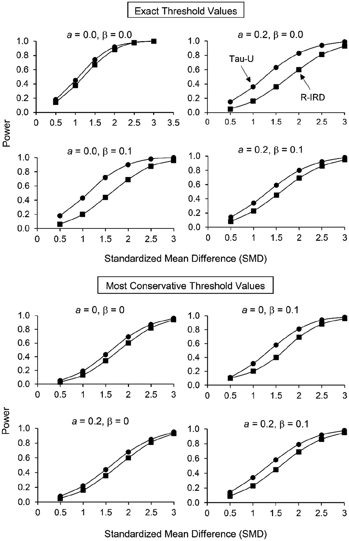
Power for the exact and most conservative threshold values for Tau-U and robust improvement rate difference for 5 points in Phase A and 10 points in Phase B. a represents the autocorrelation and β represents the trend parameter.

Discussion

Overall, our analyses show that Tau-U and R-IRD may provide adequate control over type I error rate and sufficient power when detecting changes in quasi-experimental AB designs. In addition to independently validating the properties of these measures with simulated data, our results show that the Tau-U and R-IRD can support clinical decision-making. In contrast, PEM seems inadequate as the measure is prone to ceiling effects, which inflates the type I error rate when the threshold is at 1.0. Taken together with the results obtained by Lanovaz et al. (2019), our study suggests that practitioners may adopt AB quasi-experimental design with Tau-U or R-IRD to assess individual progress while minimizing interpretation errors.

For example, a practitioner who decides to collect at least 5 data points during baseline and at least 10 data points during treatment may use 0.80 and 0.85 as thresholds for Tau-U and R-IRD, respectively (see Table 1). Observing an effect size equal to or higher than these values should produce a false positive interpretation in less than 1 in 20 cases, which is on par with the type I error rate threshold used in experimental designs. If the effect size is below the threshold, the practitioner may rely on visual analysis to provide further support. If the visual analysis shows differentiation between Phase A and Phase B, the practitioner may conduct a within-subject replication using an experimental design to confirm the results (if possible to withdraw the treatment). Otherwise (i.e., visual analysis does not show differentiation), the practitioner may conclude that there was no behavior change and assess the effects of an alternative treatment. Thus, only a small subset of individuals would require an experimental design, considerably reducing the costs and resources necessary to assess and monitor progress.

Practitioners should take into consideration the limitations of our effect size measures. First, nonoverlap measures may produce ceiling effects. When no overlap is present, the measure will indicate a large effect size (i.e., 1.0). However, this effect size only indicates the absence of overlap and does not provide information on the magnitude of the change between baseline and treatment (Ma, 2006; Parker et al., 2009). Second, the version of Tau-U used in this study is affected by the ratio of baseline to treatment data points. As such, the effect size may be artificially inflated by collecting additional treatment data points until Tau-U is statistically significant (Brossart, Laird, & Armstrong, 2018; Tarlow, 2017). If a practitioner finds a baseline trend is reducing their effect size, a within-subject replication may be warranted to confirm the effect.

Although our results are consistent with those obtained with nonsimulated data sets (Lanovaz et al., 2019) and we relied on prior research to set the values of our parameters, our simulations may not have perfectly mimicked patterns observed in practice, which is a limitation. Future research should apply the current thresholds to nonsimulated data to examine to what extent the results match those of other types of analyses (e.g., visual analyses and randomization tests). An additional limitation is that we only used nonoverlap effect size measures as part of our analyses. We could not evaluate mean-based magnitude measures such as the log response ratio (Pustejovsky, 2018) because SMD directly manipulated the mean. Therefore, inclusion of mean-based effect size measures would have produced circular outcomes.

Finally, the primary concern against the use of quasi-experimental AB designs is their inability to demonstrate functional relations (or experimental control). An experimenter has demonstrated a functional relation when an observed change was shown to be the product of an independent variable (e.g., treatment) while ruling out extraneous variables. The AB design does not rule out the effects of maturation or history (Christ, 2007), which prevents the identification of the variable responsible for an observed change. However, the AB design can determine whether the behavior (or target) has changed significantly from Phase A to Phase B, which is arguably more important for practitioners than identifying the exact mechanism responsible for this change. In sum, our results suggest that practitioners may use quasi-experimental AB designs in combination with Tau-U or R-IRD to assess and monitor progress in practice.

Supplemental Material

R_code – Supplemental material for Using AB Designs With Nonoverlap Effect Size Measures to Support Clinical Decision-Making: A Monte Carlo Validation

Supplemental material, R_code for Using AB Designs With Nonoverlap Effect Size Measures to Support Clinical Decision-Making: A Monte Carlo Validation by Antonia R. Giannakakos and Marc J. Lanovaz in Behavior Modification

Supplemental Material

Supplementary_Tables_and_Figures – Supplemental material for Using AB Designs With Nonoverlap Effect Size Measures to Support Clinical Decision-Making: A Monte Carlo Validation

Supplemental material, Supplementary_Tables_and_Figures for Using AB Designs With Nonoverlap Effect Size Measures to Support Clinical Decision-Making: A Monte Carlo Validation by Antonia R. Giannakakos and Marc J. Lanovaz in Behavior Modification

Footnotes

Declaration of Conflicting Interests

The author(s) declared no potential conflicts of interest with respect to the research, authorship, and/or publication of this article.

Funding

The author(s) disclosed receipt of the following financial support for the research, authorship, and/or publication of this article: This research project was supported, in part, by a grant from the Canadian Institutes of Health Research (#136895) and a salary award from the Fonds de Recherche du Québec—Santé (#30827) to the second author (M.J.L.).

ORCID iDs

Antonia R. Giannakakos

Marc J. Lanovaz

Supplemental Material

Supplemental material for this article is available online.

Notes

Author Biographies

Antonia R. Giannakakos, PhD, BCBA-D, LBA (CT), was a postdoctoral research fellow in the École de Psychoéducation at the Université de Montréal during this study. She is currently an assistant professor in the Special Education Department at Manhattanville College. Her research interests include staff training, childhood accident prevention, and the validity of single-case designs.

Marc J. Lanovaz, PhD, BCBA-D, is an associate professor in the École de Psychoéducation at the Université de Montréal and researcher at the Center de recherche du CHU Ste-Justine. His research interests include the assessment and treatment of challenging behavior, the use of technology to facilitate the implementation of behavioral interventions, and the validity of single-case designs.

References

Bloom

Fischer

Orme

(1999). Evaluating practice: Guidelines for the accountable professional (3rd ed.). Needham Heights, MA: Allyn & Bacon.

Brossart

D. F.

Laird

V. C.

Armstrong

T. W.

(2018). Interpreting Kendall’s Tau and Tau single-case experimental designs. Cogent Psychology, 5, 1-26. doi:10.1080/23311908.2018.1518687

Christ

T. J.

(2007). Experimental control and threats to internal validity of concurrent and nonconcurrent multiple baseline designs. Psychology in the Schools, 44, 451-459. doi:10.1002/pits.2023

Cohen

(1992). A power primer. Psychological Bulletin, 112, 155-159. doi:10.1037/0033-2909.112.1.155

Engel

R. J.

Schutt

R. K.

(2017). Single-subject design. In Engel

R. J.

Schutt

R. K.

(Eds.), The practice of research in social work (pp. 206-246). New York, NY: SAGE.

Fisher

W. W.

Kelley

M. E.

Lomas

J. E.

(2003). Visual aids and structured criteria for improving visual inspection and interpretation of single-case designs. Journal of Applied Behavior Analysis, 36, 387-406. doi:10.1901/jaba.2003.36-387

Foster

L. H.

Watson

Meeks

Young

J. S.

(2002). Single-subject research design for school counselors: Becoming an applied researcher. Professional School Counseling, 6, 146-154.

Gierut

J. A.

Morrisette

M. L.

Dickinson

S. L.

(2015). Effect size for single-subject design in phonological treatment. Journal of Speech, Language, and Hearing Research, 58, 1464-1481. doi:10.1044/2015_JSLHR-S-14-0299

Hayes

S. C.

(1981). Single case design and empirical clinical practice. Journal of Consulting and Clinical Psychology, 49, 193-211. doi:10.1037/0022-006X.49.2.193

10.

Janosky

J. E.

Leininger

S. L.

Hoerger

M. P.

Libkuman

T. M.

(2009). Ethics and single-subject research. In Janosky

J. E.

Hoerger

M. P.

Libkuman

T. M.

Leininger

S. L.

(Eds.), Single subject designs in biomedicine (pp. 69-80). Dordrecht, The Netherlands: Springer.

11.

Kratochwill

T. R.

Hitchcock

Horner

R. H.

Levin

J. R.

Odom

S. L.

Rindskopf

D. M.

Shadish

W. R.

(2010). Single-case designs technical documentation. Retrieved from http://files.eric.ed.gov/fulltext/ED510743.pdf

12.

Lanovaz

M. J.

Turgeon

Cardinal

Wheatley

T. L.

(2019). Using single-case designs in practical settings: Is within-subject replication always necessary? Perspectives on Behavior Science, 42, 153-162. doi:10.1007/s40614-018-0138-9

13.

Lundervold

D. A.

Belwood

M. F.

(2011). The best kept secret in counseling: Single-case (N=1) experimental designs. Journal of Counseling & Development, 78, 92-102. doi:10.1002/j.1556-6676.2000.tb02565.x

14.

H.-H.

(2006). An alternative method for quantitative synthesis of single-subject researchers: Percentage of data points exceeding the median. Behavior Modification, 30, 598-617. doi:10.1177/0145445504272974

15.

Machalicek

Horner

H. H.

(2018). Special issue on advances in single-case research design and analysis. Developmental Neurorehabilitation, 21, 209-211. doi:10.1080/17518423.2018.1468600

16.

Manolov

Sierra

Solanas

Botella

(2014). Assessing functional relations in single-case designs: Quantitative proposals in the context of the evidence-based movement. Behavior Modification, 38, 878-913. doi:10.1177/0145445514545679

17.

Nugent

W. R.

(2001). Single case design visual analysis procedures for use in practice evaluation. Journal of Social Service Research, 27, 39-75. doi:10.1300/J079v27n02_03

18.

Odom

S. L.

Brantlinger

Gersten

Horner

R. H.

Thompson

Harris

K. R.

(2005). Research in special education: Scientific methods and evidence-based practice. Exceptional Children, 71, 137-148. doi:10.1177/001440290507100201

19.

Parker

R. I.

Hagan-Burke

Vannest

(2007). Percentage of all non-overlapping data (PAND): An alternative to PND. The Journal of Special Education, 40, 194-204. doi:10.1177/00224669070400040101

20.

Parker

R. I.

Vannest

K. J.

Brown

(2009). The improvement rate difference for single-case research. Exceptional Children, 75, 135-150. doi:10.1177/001440290907500201

21.

Parker

R. I.

Vannest

K. J.

Davis

J. L.

(2011). Effect size in single-case research: A review of nine nonoverlap techniques. Behavior Modification, 35, 303-322. doi:10.1177/0145445511399147

22.

Pustejovsky

J. E.

(2017). Single-case effect size calculator [Version 0.2; Web application]. Retrieved from https://jepusto.shinyapps.io/SCD-effect-sizes/

23.

Pustejovsky

J. E.

(2018). Procedural sensitivities of effect sizes for single-case designs with directly observed behavioral outcomes. Psychological Methods, 24, 217-235. doi:10.1037/met0000179

24.

Rogers

L. A.

Graham

(2008). A meta-analysis of single subject design writing intervention research. Journal of Educational Psychology, 100, 879-906. doi:10.1037/0022-0663.100.4.87

25.

Shadish

W. R.

Sullivan

K. J.

(2011). Characteristics of single-case designs used to assess intervention effects in 2008. Behavior Research Methods, 43, 971-980. doi:10.3758/s13428-011-0111-y

26.

Tarlow

(2017). An improved rank correlation effect size statistic for single-case designs: Baseline corrected tau. Behavior Modification, 41, 427-467. doi:10.1177/0145445516676750

27.

Vannest

K. J.

Ninci

(2015). Evaluating intervention effects in single-case research designs. Journal of Counseling & Development, 93, 403-411. doi:10.1002/jcad.12038

Supplementary Material

Please find the following supplemental material available below.

For Open Access articles published under a Creative Commons License, all supplemental material carries the same license as the article it is associated with.

For non-Open Access articles published, all supplemental material carries a non-exclusive license, and permission requests for re-use of supplemental material or any part of supplemental material shall be sent directly to the copyright owner as specified in the copyright notice associated with the article.

0.00 MB

0.01 MB

0.66 MB