Intelligence,Birth Order,and Family Size

Abstract

The analysis of the National Child Development Study in the United Kingdom (n = 17,419) replicates some earlier findings and shows that genuine within-family data are not necessary to make the apparent birth-order effect on intelligence disappear. Birth order is not associated with intelligence in between-family data once the number of siblings is statistically controlled. The analyses support the admixture hypothesis, which avers that the apparent birth-order effect on intelligence is an artifact of family size, and cast doubt on the confluence and resource dilution models, both of which claim that birth order has a causal influence on children’s cognitive development. The analyses suggest that birth order has no genuine causal effect on general intelligence.

Keywords

birth-order effect intelligence admixture hypothesis confluence model resource dilution model

The birth-order effect on intelligence—whether a child’s birth order among siblings causally influences its intelligence—has long been hotly debated ever since Galton (1874) noticed a preponderance of firstborns among eminent English scientists nearly a century and a half ago. A recent review notes that “research on birth order and intellectual performance is replete with contradictory findings and long-standing conceptual disagreements” (Sulloway, 2007, p. 1711).

On the one hand, the confluence model (Zajonc, 1976; Zajonc & Markus, 1975; Zajonc & Mullally, 1997) and the resource dilution model (Blake, 1981; Downey, 2001) suggest that the average intelligence of children should decline with increasing birth order, such that firstborns are on average more intelligent than secondborns, and secondborns are on average more intelligent than thirdborns. According to the confluence model, firstborns are born into a family that consists entirely of cognitively mature adults; secondborns are born into a family that consists of 67% cognitively mature adults; thirdborns are born into a family that consists only of 50% cognitively mature adults. Hence, the higher their birth order, the less cognitively stimulating the children’s family environment. Similarly, the resource dilution model points out that parents’ material resources, energy, and attention are all finite, and thus the more children there are in the family, the less of each resource necessarily accrues to each child. The higher-order offspring (laterborns) are therefore expected to suffer from such relative lack of resources in the family and thus to attain lower intelligence, among other things.

In sharp contrast, the admixture hypothesis (Page & Grandon, 1979; Rodgers, 2001; Rodgers, Cleveland, van den Oord, & Rowe, 2000) suggests that the apparent birth-order effect on intelligence is a methodological artifact of using between-family (cross-sectional) data to infer within-family dynamics. It explains the correlation between birth order and intelligence across individuals by the fact that (a) less intelligent parents are more likely to have a larger number of children and (b) higher birth-order children necessarily come from larger families, whereas children from smaller families have greater representation among lower birth-order children. For example, fourthborns necessarily come from families with four or more children, whereas firstborns can come either from families with one or two children or families with five or six children. Given the preponderance of families with a small number of children, such families are overrepresented in samples of first- and secondborns. Thus, if there is a negative correlation between parental intelligence and their number of children, then it can create a statistical association between birth order and intelligence among children across families.

The debate over the genuine causal effect of birth order on intelligence remains unresolved (Sulloway, 2007). At the heart of the disagreements between the confluence/resource dilution models and the admixture hypothesis is the question of whether the birth-order effect on intelligence—where laterborns are on average less intelligent than earlierborns—reflects a genuine within-family dynamic, or a spurious artifact and methodological confound of inferring a within-family process from between-family data, of comparing laterborns from larger families with earlierborns from smaller families. The confluence/resource dilution models contend that earlierborns are on average more intelligent than laterborns within the same families, whereas the admixture hypothesis contends that children of any birth order from smaller families are on average more intelligent than children of any birth order from larger families.

One empirical generalization that emerges in the debate on intelligence and birth order is that studies using between-family data (comparing individuals with given birth orders from different families) typically find a statistically significant association between birth order and intelligence (Boomsma et al., 2008; Zajonc & Bargh, 1980), whereas studies using within-family data (comparing siblings within the same families) typically do not (Retherford & Sewell, 1991; Rodgers et al., 2000), although a few within-family studies have found a birth-order effect (Belmont & Marolla, 1973; Bjerkedal, Kristensen, Skjeret, & Brevik, 2007; Record, McKeown, & Edwards, 1969).

Most recently, Bjerkedal et al. (2007) used population data on a quarter of a million Norwegian male conscripts born between 1967 and 1998 (84.7% of all males born in these years) to provide both between-family and within-family comparisons simultaneously. Their analyses show that birth order and sibship size have independent and simultaneous effects on intelligence. Boys of a given birth order become less intelligent as their sibship size increases, and sons from the same families become less intelligent as their birth order increases.

In an attempt to resolve the “birth order puzzle,” where some within-family studies show a negative effect of birth order (earlierborns are more intelligent than laterborns) while others show a positive effect (laterborns are more intelligent than earlierborns), Zajonc, Markus, and Markus (1979) revised the original confluence model (Zajonc, 1976; Zajonc & Markus, 1975) to incorporate the “tutoring effect.” They argue that firstborns initially suffer in their intellectual development at the birth of the secondborn, because the intellectually and verbally less mature secondborn degrades the level of intellectual stimulation of the family environment. However, firstborns later recover from the temporary deficit by being able to tutor the second- and laterborns, whereas lastborns never have the opportunity to tutor younger siblings. The revised confluence model predicts that firstborns are less intelligent than laterborns until about the age of 12, but firstborns become more intelligent than laterborns after 12.

The confluence/resource dilution models and the admixture hypothesis make clear and divergent predictions on the relationship between intelligence, birth order, and family size in between-family data. Both confluence/resource dilution models and the admixture hypothesis predict a significant negative bivariate association between birth order and intelligence in between-family data. However, the confluence/resource dilution models predict that birth order has a genuine causal effect on intelligence, and thus birth order is negatively associated with intelligence even net of family size. In sharp contrast, the admixture hypothesis predicts that the negative association between birth order and intelligence is spurious and disappears once family size is statistically controlled.

Empirical Analyses

Data

The National Child Development Study (NCDS) is a large-scale prospectively longitudinal study which has followed a population of British respondents since birth for more than half a century. The study includes all babies (n = 17,419) born in Great Britain (England, Wales, and Scotland) during 1 week (March 03-09, 1958). The respondents are subsequently reinterviewed in 1965 (Sweep 1 at Age 7; n = 15,496), in 1969 (Sweep 2 at Age 11; n = 18,285), in 1974 (Sweep 3 at Age 16; n = 14,469), in 1981 (Sweep 4 at Age 23; n = 12,537), in 1991 (Sweep 5 at Age 33; n = 11,469), in 1999-2000 (Sweep 6 at Age 41-42; n = 11,419), and in 2004-2005 (Sweep 7 at Age 46-47; n = 9,534). There are more respondents in Sweep 2 than in the original sample (Sweep 0) because Sweep 2 sample includes eligible children who were in the country in 1969 but not in 1958 when Sweep 0 interviews were conducted. In each sweep, personal interviews and questionnaires are administered to the respondents, to their mothers, teachers, and doctors during childhood, and to their partners and children in adulthood. Virtually all (97.8%) of the NCDS respondents are Caucasian.

Measure of General Intelligence

The NCDS respondents take multiple intelligence tests at Ages 7, 11, and 16. At 7, the respondents take four cognitive tests (Copying Designs Test, Draw-a-Man Test, Southgate Group Reading Test, and Problem Arithmetic Test). At 11, they take five cognitive tests (Verbal General Ability Test, Nonverbal General Ability Test, Reading Comprehension Test, Mathematical Test, and Copying Designs Test). At 16, they take two cognitive tests (Reading Comprehension Test and Mathematics Comprehension Test). Appendix Table 1 presents the means, standard deviations, and full correlation matrix for the 11 test scores.

I first perform a principal components analysis at each age to compute their general intelligence score for each age. Each principal components analysis uses a varimax rotation and an extraction criterion of minimum eigenvalue of 1.0. I perform all statistical analyses with SPSS 19.0 for Macintosh.

All cognitive test scores at each age load only on one component, with reasonably high loadings (Age 7: Copying Designs = .671, Draw-a-Man = .696, Southgate Group Reading = .780, and Problem Arithmetic = .762; Age 11: Verbal General Ability = .920, Nonverbal General Ability = .885, Reading Comprehension = .864, Mathematical = .903, and Copying Designs = .486; and Age 16: Reading Comprehension = .909, and Mathematics Comprehension = .909). For Age 7, the extracted component has the eigenvalue of 2.123 and explains 53.081% of the variance. For Age 11, the extracted component has the eigenvalue of 3.428 and explains 68.553% of the variance. For Age 16, the extracted component has the eigenvalue of 1.654 and explains 82.697% of the variance.

The extracted component at each age has a mean of 0 and a standard deviation of 1.0. It is then converted into the standard IQ metric, with a mean of 100 and a standard deviation of 15 (Conversion formula: IQ = 100 + 15 × component). Then I perform a second-order principal components analysis with the IQ scores at three different ages to compute the overall childhood general intelligence score. The three IQ scores load only on one component with very high factor loadings (Age 7 = .867; Age 11 = .947; Age 16 = .919). The extracted component has the eigenvalue of 2.491 and explains 83.031% of the variance. I use the childhood general intelligence score in the standard IQ metric as a measure of childhood general intelligence.

The measure of childhood general intelligence thus constructed via principal components analysis correlates extremely highly with some possible alternative measures. For example, if I standardize each of the 11 test scores at three ages and take a grand mean, it correlates r = .995 with the measure of childhood general intelligence constructed via principal components analysis. If I simply add all the 11 raw test scores, it correlates r = .991. As a result, all of my substantive conclusions below remain virtually identical regardless of which alternative measure of childhood general intelligence I use.

Control Variables

In addition to birth order and number of siblings, both measured at 16, I control for the following variables in my multiple regression analyses below: social class at birth measured by father’s occupational class: 0 = unemployed, dead, retired, or no father present; 1 = unskilled; 2 = semiskilled; 3 = skilled; 4 = white collar; 5 = professional); mother’s education; father’s education (both measured at 16 as the age at which the parent left full-time education on the ordinal scale: 1 = younger than 13; 2 = 13-14; 3 = 14-15; 4 = 15-16; 5 = 16-17; 6 = 17-18; 7 = 18-19; 8 = 19-21; 9 = 21-23; and 10 = older than 23). Measures of parental intelligence are not available in NCDS.

Lassek and Gaulin (2008) showed that mother’s gluteofemoral (lower-body) fat increases their children’s cognitive ability, and shorter birth interval may deplete the mother’s reserve of such developmentally beneficial body fat. So I further control for the birth interval, measured at birth, as the number of years since previous birth (1 = less than a year; 2 = 1-2 years; 3 = 2-3 years; 4 = 3-4 years; 5 = 4-5 years; 6 = 5-10 years; 8 = 15-20 years; 9 = more than 20 years). Firstborns are assigned the arbitrary value of 9 for this variable; however, all of my substantive conclusions from the regression model that includes birth interval remain identical if I exclude firstborns from the analysis.

Finally, Kohler, Rodgers, and Christensen (1999) showed that fertility may partly be heritable; the more children one has, the more children one’s children are genetically predisposed to have. I therefore control for the number of mother’s siblings, measured at birth.

Results

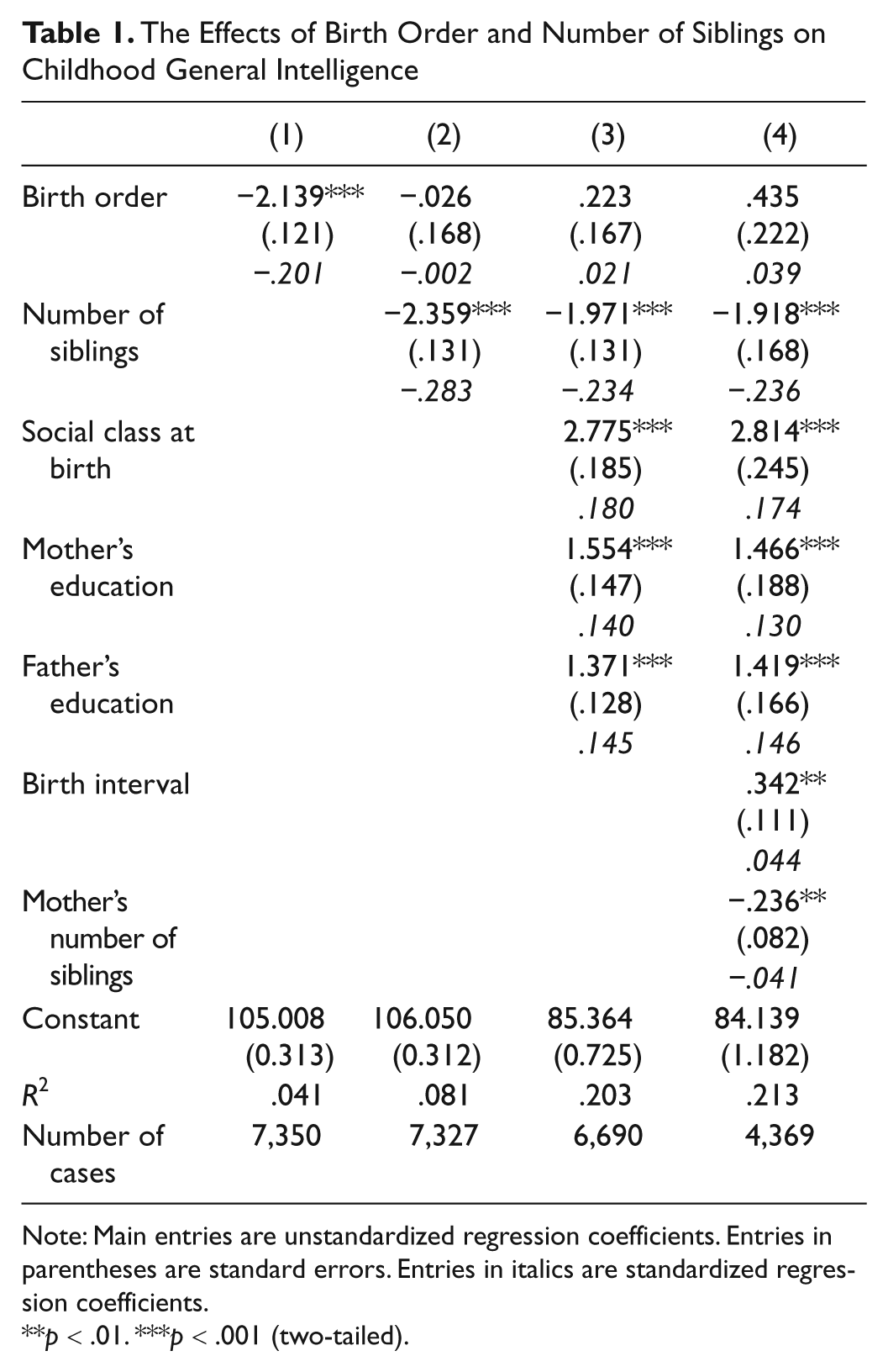
Table 1 presents the results of multiple regression analyses of the NCDS data. Appendix Table 2 presents the full correlation matrix, with means and standard deviations, for all the variables used in the multiple regression analyses. Online supplemental material (available at http://pspb.sagepub.com/supplemental) presents, both in tables and figures, mean IQ: (a) by birth order (Table S1 and Figure S1), (b) by number of siblings (Table S2 and Figure S2), and (c) by birth order, by number of siblings (Table S3 and Figure S3). It also presents mean IQ by lifetime number of children (Table S4 and Figure S4).

Table 1.

The Effects of Birth Order and Number of Siblings on Childhood General Intelligence

	(1)	(2)	(3)	(4)
Birth order	−2.139*** (.121)	−.026 (.168)	.223 (.167)	.435 (.222)
Birth order	−.201	−.002	.021	.039
Number of siblings		−2.359*** (.131)	−1.971*** (.131)	−1.918*** (.168)
Number of siblings		−.283	−.234	−.236
Social class at birth			2.775*** (.185)	2.814*** (.245)
Social class at birth			.180	.174
Mother’s education			1.554*** (.147)	1.466*** (.188)
Mother’s education			.140	.130
Father’s education			1.371*** (.128)	1.419*** (.166)
Father’s education			.145	.146
Birth interval				.342** (.111)
Birth interval				.044
Mother’s number of siblings				−.236** (.082)
Mother’s number of siblings				−.041
Constant	105.008 (0.313)	106.050 (0.312)	85.364 (0.725)	84.139 (1.182)
R ²	.041	.081	.203	.213
Number of cases	7,350	7,327	6,690	4,369

Note: Main entries are unstandardized regression coefficients. Entries in parentheses are standard errors. Entries in italics are standardized regression coefficients.

p < .01. ***p < .001 (two-tailed).

Column (1) shows that, consistent with the past studies on the birth-order effect on intelligence with between-family data, there is a significant negative association between birth order and childhood general intelligence (b = −2.139, p < .001, standardized coefficient = −.201). The unstandardized regression coefficient of −2.139 for birth order appears to suggest that NCDS respondents lose more than 2 IQ points for each position in the birth order. Although earlier studies suggest that the birth-order effect on parental investment may be quadratic, such that firstborns and lastborns receive more parental investment than middleborns (Hertwig, Davis, & Sulloway, 2002; Salmon & Daly, 1998), the association between intelligence and birth order does not deviate from linearity (b for birth order squared = −.023, ns, standardized coefficient = −.016).

Column (2) shows, however, that, once I control for the number of siblings in the family, birth order is no longer significantly associated with childhood general intelligence (b = −.026, ns, standardized coefficient = −.002). In sharp contrast, the number of siblings is significantly negatively associated with childhood general intelligence (b = −2.359, p < .001, standardized coefficient = −.283). The unstandardized regression coefficient of −2.359 suggests that NCDS respondents with the same birth order lose 2.4 IQ points for each sibling in the family. Naturally, birth order and the number of siblings are very strongly positively correlated (r = .700, p < .001, n = 11,450; see appendix Table 2). However, the correlation is not strong enough to cause collinearity (VIF for both variables = 1.971).

Column (3) shows that including controls for the respondent’s social class background (father’s occupational status, mother’s education, father’s education) in the equation does not alter the conclusion at all and only very slightly attenuates the association between number of siblings and childhood general intelligence (b = −1.971, p < .001, standardized coefficient = −.234). Even though all variables included in this equation, except for birth order, are significantly associated with childhood general intelligence, a comparison of standardized regression coefficients suggests that number of siblings has the strongest association.

Column (4) shows that further controlling for birth interval and mother’s number of siblings does not alter the main conclusion or attenuate the association between number of siblings and childhood general intelligence. Once again, even though all variables included in this equation, except for birth order, are significantly associated with childhood general intelligence, a comparison of standardized regression coefficients suggests that number of siblings has the strongest association (−.236).

Because NCDS measures respondents’ intelligence at Ages 7, 11, and 16, it allows for a direct test of the “tutoring effect” posited by the confluence model (Zajonc et al., 1979) and see if laterborns are on average more intelligent than earlierborns until about the age of 12 but earlierborns become more intelligent than laterborns after 12.

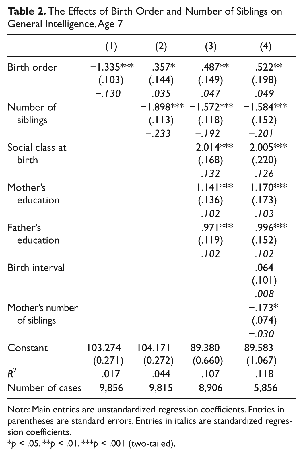
Results presented in Tables 2 to 4 provide very little support for the “tutoring effect” and for the confluence model. Table 2, Column (1), shows that, even as early as 7, earlierborns are significantly more intelligent than laterborns (b = −1.335, p < .001, standardized coefficient = −.130), contrary to the revised prediction of the confluence model. It is only when I control for the number of siblings that the association between birth order and general intelligence becomes significantly positive (b = .357, p < .05, standardized coefficient = .035). However, number of children has a much stronger association with general intelligence at 7 than birth order does. Net of each other, each additional sibling decreases general intelligence by 1.9 IQ points, whereas each position in birth order only increases it by 0.4 IQ points.

Table 2.

The Effects of Birth Order and Number of Siblings on General Intelligence, Age 7

	(1)	(2)	(3)	(4)
Birth order	−1.335*** (.103)	.357* (.144)	.487** (.149)	.522** (.198)
Birth order	−.130	.035	.047	.049
Number of siblings		−1.898*** (.113)	−1.572*** (.118)	−1.584*** (.152)
Number of siblings		−.233	−.192	−.201
Social class at birth			2.014*** (.168)	2.005*** (.220)
Social class at birth			.132	.126
Mother’s education			1.141*** (.136)	1.170*** (.173)
Mother’s education			.102	.103
Father’s education			.971*** (.119)	.996*** (.152)
Father’s education			.102	.102
Birth interval				.064 (.101)
Birth interval				.008
Mother’s number of siblings				−.173* (.074)
Mother’s number of siblings				−.030
Constant	103.274 (0.271)	104.171 (0.272)	89.380 (0.660)	89.583 (1.067)
R ²	.017	.044	.107	.118
Number of cases	9,856	9,815	8,906	5,856

Note: Main entries are unstandardized regression coefficients. Entries in parentheses are standard errors. Entries in italics are standardized regression coefficients.

p < .05. **p < .01. ***p < .001 (two-tailed).

Table 3.

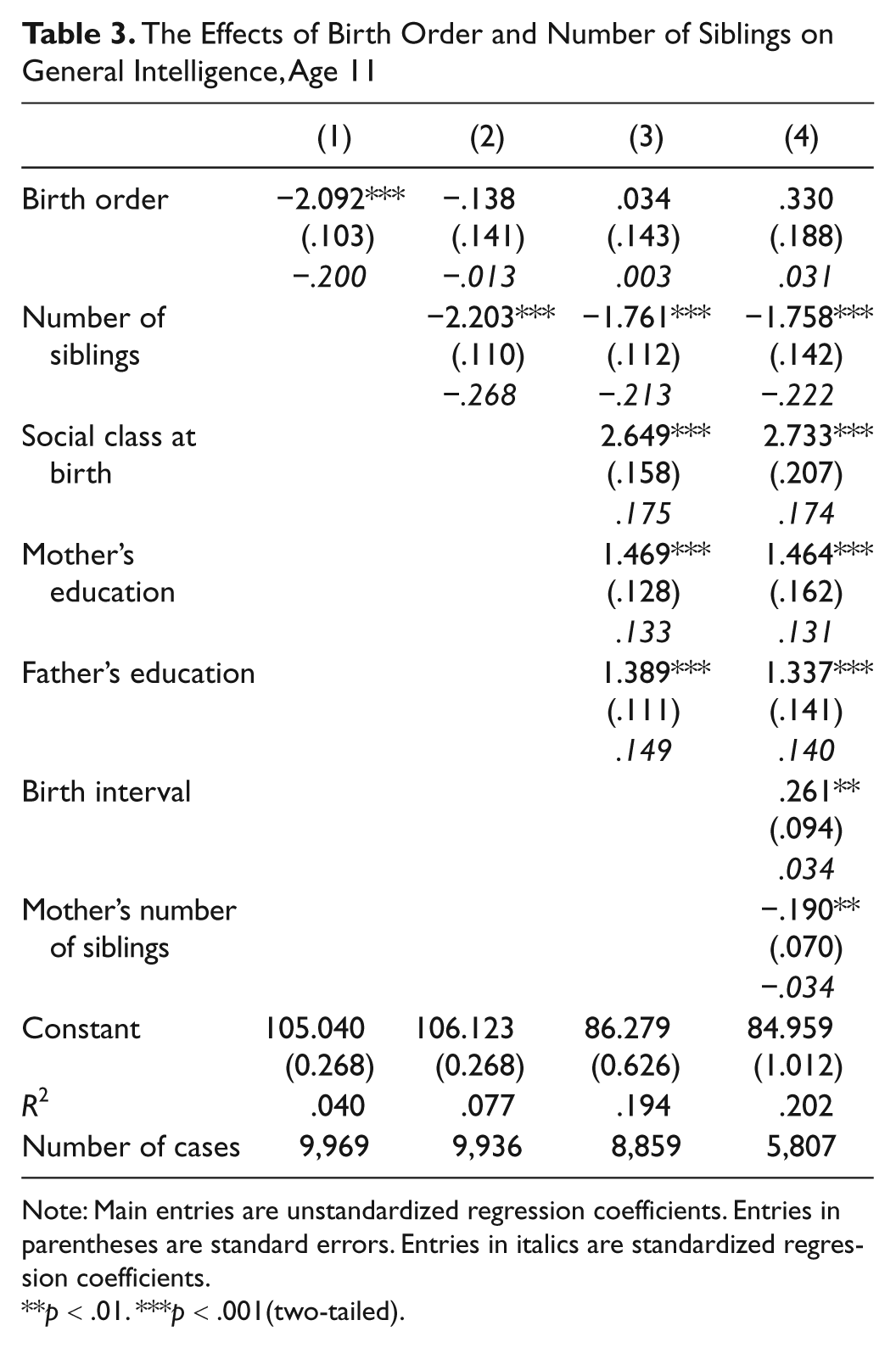
The Effects of Birth Order and Number of Siblings on General Intelligence, Age 11

	(1)	(2)	(3)	(4)
Birth order	−2.092*** (.103)	−.138 (.141)	.034 (.143)	.330 (.188)
Birth order	−.200	−.013	.003	.031
Number of siblings		−2.203*** (.110)	−1.761*** (.112)	−1.758*** (.142)
Number of siblings		−.268	−.213	−.222
Social class at birth			2.649*** (.158)	2.733*** (.207)
Social class at birth			.175	.174
Mother’s education			1.469*** (.128)	1.464*** (.162)
Mother’s education			.133	.131
Father’s education			1.389*** (.111)	1.337*** (.141)
Father’s education			.149	.140
Birth interval				.261** (.094)
Birth interval				.034
Mother’s number of siblings				−.190** (.070)
Mother’s number of siblings				−.034
Constant	105.040 (0.268)	106.123 (0.268)	86.279 (0.626)	84.959 (1.012)
R ²	.040	.077	.194	.202
Number of cases	9,969	9,936	8,859	5,807

Note: Main entries are unstandardized regression coefficients. Entries in parentheses are standard errors. Entries in italics are standardized regression coefficients.

p < .01. ***p < .001(two-tailed).

Table 4.

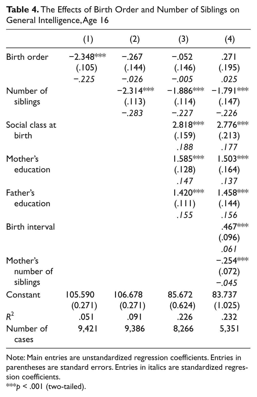
The Effects of Birth Order and Number of Siblings on General Intelligence, Age 16

	(1)	(2)	(3)	(4)
Birth order	−2.348*** (.105)	−.267 (.144)	−.052 (.146)	.271 (.195)
	−.225	−.026	−.005	.025
Number of siblings		−2.314*** (.113)	−1.886*** (.114)	−1.791*** (.147)
		−.283	−.227	−.226
Social class at birth			2.818*** (.159)	2.776*** (.213)
			.188	.177
Mother’s education			1.585*** (.128)	1.503*** (.164)
			.147	.137
Father’s education			1.420*** (.111)	1.458*** (.144)
			.155	.156
Birth interval				.467*** (.096)
				.061
Mother’s number of siblings				−.254*** (.072)
Mother’s number of siblings				−.045
Constant	105.590 (0.271)	106.678 (0.271)	85.672 (0.624)	83.737 (1.025)
R ²	.051	.091	.226	.232
Number of cases	9,421	9,386	8,266	5,351

Note: Main entries are unstandardized regression coefficients. Entries in parentheses are standard errors. Entries in italics are standardized regression coefficients.

***

p < .001 (two-tailed).

Table 3 shows that, contrary to the prediction of the confluence model, laterborns are not significantly more intelligent than earlierborns at 11. Nor are earlierborns more intelligent than laterborns at 16, as Table 4 shows. In general, the results presented in Tables 2 to 4 largely replicate the findings in Table 1 and support the admixture hypothesis. At each age, number of siblings is significantly negatively associated with childhood general intelligence, and its association is the strongest of all the variables included in the equation.

Discussion

I use prospectively longitudinal between-family data with a large population of respondents (the NCDS in the United Kingdom) to test competing predictions from the confluence/resource dilution models and the admixture hypothesis on the effect of birth order on intelligence. The NCDS has one of the strongest measures of general intelligence in any survey data, assessed by 11 cognitive tests at three different ages. Multiple regression analyses indicate that the apparent birth-order effect on intelligence is an artifact of the association between intelligence and family size, as the admixture hypothesis contends. The study is among the first (along with Wichman, Rodgers, & MacCallum, 2006) to show that the apparent and statistically significant birth-order effect on intelligence in between-family data completely disappears once one between-family variable is statistically controlled.

The admixture hypothesis is based on the premise that more intelligent parents on average have fewer children than less intelligent parents. In the NCDS data, childhood general intelligence is weakly but statistically significantly associated with the lifetime number of children before 47 (r = −.038, p < .01, n = 4,973; see Table S4 and Figure S4 in the supplemental material available at http://pspb.sagepub.com/supplemental). But why should this be so? Why do more intelligent parents have fewer children?

There has been some evidence that, because general intelligence likely evolved to solve evolutionarily novel problems, more intelligent individuals are more likely to acquire and espouse evolutionarily novel preferences and values than less intelligent individuals (Kanazawa, 2010a, 2010b, 2012). Humans, just like all other biological species, are evolutionarily designed to maximize their reproductive success, and thus voluntary control of fertility—having fewer children than one can safely raise to sexual maturity—is an evolutionarily novel value. Hence, more intelligent individuals may be more likely than less intelligent individuals to adopt the evolutionarily novel value of having fewer children. At the same time, there is some evidence that, because all forms of contraception (except for abstinence) are evolutionarily novel, more intelligent individuals may be better able to implement them more effectively than less intelligent individuals (Kanazawa, 2005). I should point out, however, that there is no consensus on the evolutionary functions of general intelligence. Some (Chiappe & MacDonald, 2005; Cosmides & Tooby, 2002) believe it is a truly domain-general evolved psychological mechanism, whereas others (Miller, 2000) equate it with mating intelligence.

Past studies on the possible effect of birth order on intelligence suggest that between-family data, comparing children from different families, show a significantly negative association between intelligence and birth order, whereas within-family data, comparing siblings from the same families, do not. How, then, can I reconcile my results above with Bjerkedal et al.’s (2007) findings with within-family data that secondborn sons on average are less intelligent than their firstborn brothers by 2.3 IQ points, and that third-born sons on average are less intelligent than their secondborn brothers by 1.1 IQ points?

For the most part, Bjerkedal et al. (2007) used standardized intelligence test scores in all of their analyses; raw scores on the general ability tests (in the range of 1 to 9) are standardized within each age and calendar year. Bjerkedal et al. (2007) noted that there was a secular increase in average intelligence in Norway from 1985 through the early 1990s. The oldest cohort of men in Bjerkedal et al.’s data were born in 1967 and thus turned 18 in 1985, when they became eligible for conscription and took the compulsory military board cognitive test. If two brothers receive exactly the same raw score on the general ability test, then the younger brother will have a lower standardized score in the face of the secular rise in average intelligence. To what extent Bjerkedal et al.’s finding of within-family birth-order effects reflects the methodological artifact of using standardized scores rather than raw scores remains unclear. Further studies taking advantage of high-quality, population-based within-family data are clearly necessary to adjudicate between conflicting findings and to discover whether a genuine birth-order effect on intelligence exists within families.

The analysis of the NCDS in the United Kingdom shows that genuine within-family data are not necessary to make the apparent birth-order effect on intelligence disappear. Although both birth order and number of siblings are negatively associated with childhood general intelligence on their own, birth order is no longer significantly associated with intelligence once sibship size is controlled. Number of siblings consistently has the strongest association with childhood general intelligence in all of the multiple regression equations. However, I hasten to add that the effect of number of siblings on intelligence, while the largest of all variables included in all models, is still relatively small, with the effect size in the range of .20 to .28. I encourage other researchers to construct and test alternative, theoretically motivated models with different sets of covariates to examine the relative effects of birth order and number of siblings on childhood general intelligence.

The analyses presented above provide strong empirical support for the admixture hypothesis and suggest that the apparent birth-order effect on intelligence may be a methodological artifact. They are also consistent with Wichman et al.’s (2006; but see Zajonc & Sulloway, 2007, and Wichman, Rodgers, & MacCallum, 2007) finding, using a multilevel model, that the birth-order effect on intelligence disappears once one between-family variable—mother’s age at the birth of first child—is controlled. The analyses of the NCDS data suggest that past between-family studies found a birth-order effect on intelligence because it did not control for family size (or parental intelligence). The results presented here confirm Rodgers et al.’s (2000) conclusion that “although low-IQ parents have been making large families, large families do not make low-IQ children in modern U.S. society” (p. 599) and extend it to modern British society.

Footnotes

Appendix

Acknowledgements

I thank Chi-chia Jessica Cheng, Jeremy Freese, Gordon G. Gallup, Jr., Joseph Lee Rodgers, Catherine A. Salmon, Todd K. Shackelford, Frank J. Sulloway, Associate Editor M. Brent Donnellan, and anonymous reviewers for their comments on earlier drafts.

Declaration of Conflicting Interests

The author declared the following potential conflicts of interest with respect to the research, authorship, and/or publication of this article: The author is a firstborn.

Funding

The author received no financial support for the research, authorship, and/or publication of this article.

References

Belmont

Marolla

F. A.

(1973). Birth order, family size, and intelligence. Science, 182, 1096-1101.

Bjerkedal

Kristensen

Skjeret

G. A.

Brevik

J. I.

(2007). Intelligence test scores and birth order among young Norwegian men (conscripts) analyzed within and between families. Intelligence, 35, 503-514.

Blake

(1981). Family size and the quality of children. Demography, 18, 421-442.

Boomsma

D. I.

van Beijsterveld

T. C. E. M.

Beem

A. L.

Hoekstra

R. A.

Polderman

T. J. C.

Bartels

(2008). Intelligence and birth order in boys and girls. Intelligence, 36, 630-634.

Chiappe

MacDonald

(2005). The evolution of domain-general mechanisms in intelligence and learning. Journal of General Psychology, 132, 5-40.

Cosmides

Tooby

(2002). Unraveling the enigma of human intelligence: Evolutionary psychology and the multimodular mind. In Sternberg

R. J.

Kaufman

J. C.

(Eds.), The evolution of intelligence (pp. 145-198). Mahwah, NJ: Lawrence Erlbaum.

Downey

D. B.

(2001). Number of siblings and intellectual development: The resource dilution explanation. American Psychologist, 56, 497-504.

Galton

(1874). English men of science: Their nature and nurture. London, England: Macmillan.

Hertwig

Davis

J. N.

Sulloway

F. J.

(2002). Parental investment: How an equity motive can produce inequality. Psychological Bulletin, 128, 728-745.

10.

Kanazawa

(2005). An empirical test of a possible solution to the central theoretical problem of human sociobiology. Journal of Cultural and Evolutionary Psychology, 3, 255-266.

11.

Kanazawa

(2010a). Evolutionary psychology and intelligence research. American Psychologist, 65, 279-289.

12.

Kanazawa

(2010b). Why liberals and atheists are more intelligent. Social Psychology Quarterly, 73, 33-57.

13.

Kanazawa

(2012). The intelligence paradox: Why the intelligent choice isn’t always the smart one. New York, NY: John Wiley.

14.

Kohler

H.-P.

Rodgers

J. L.

Christensen

(1999). Is fertility behavior in our genes? Findings from a Danish twin study. Population and Development Review, 25, 253-288.

15.

Lassek

W. D.

Gaulin

S. J. C.

(2008). Waist-hip ratio and cognitive ability: Is gluteofemoral fat a privileged store of neurodevelopmental resources? Evolution & Human Behavior, 29, 26-34.

16.

Miller

G. F.

(2000). Sexual selection for indicators of intelligence. In Bock

G. R.

Goode

J. A.

Webb

(Eds.), The nature of intelligence (pp. 260-275). New York, NY: John Wiley.

17.

Page

E. B.

Grandon

(1979). Family configuration and mental ability: Two theories contrasted with U.S. data. American Educational Research Journal, 16, 257-272.

18.

Record

R. G.

McKeown

Edwards

J. H.

(1969). The relation of measured intelligence to birth order and maternal age. Annals of Human Genetics, 33, 61-69.

19.

Retherford

R. D.

Sewell

W. H.

(1991). Birth order and intelligence: Further tests of the confluence model. American Sociological Review, 56, 141-158.

20.

Rodgers

J. L.

(2001). What causes birth order–intelligence pattern? The admixture hypothesis, revived. American Psychologist, 56, 505-510.

21.

Rodgers

J. L.

Cleveland

H. H.

van den Oord

Rowe

D. C.

(2000). Resolving the debate over birth order, family size, and intelligence. American Psychologist, 55, 599-612.

22.

Salmon

C. A.

Daly

(1998). Birth order and familial sentiment: Middleborns are different. Evolution & Human Behavior, 19, 299-312.

23.

Sulloway

F. J.

(2007). Birth order and intelligence. Science, 317, 1711-1712.

24.

Wichman

A. L.

Rodgers

J. L.

MacCallum

R. C.

(2006). A multilevel approach to the relationship between birth order and intelligence. Personality and Social Psychology Bulletin, 32, 117-127.

25.

Wichman

A. L.

Rodgers

J. L.

MacCallum

R. C.

(2007). Birth order has no effect on intelligence: A reply and extension of previous findings. Personality and Social Psychology Bulletin, 33, 1195-1200.

26.

Zajonc

R. B.

(1976). Family configuration and intelligence. Science, 192, 227-236.

27.

Zajonc

R. B.

Bargh

(1980). The confluence model: Parameter estimation in six divergent data sets on family factors and intelligence. Intelligence, 4, 349-361.

28.

Zajonc

R. B.

Markus

G. B.

(1975). Birth order and intellectual development. Psychological Review, 82, 74-88.

29.

Zajonc

R. B.

Markus

G. B.

(1979). The birth order puzzle. Journal of Personality and Social Psychology, 37, 1325-1341.

30.

Zajonc

R. B.

Mullally

P. R.

(1997). Birth order: Reconciling conflicting effects. American Psychologist, 52, 685-699.

31.

Zajonc

R. B.

Sulloway

F. J.

(2007). The confluence model: Birth order as a within-family or between-family dynamic? Personality and Social Psychology Bulletin, 33, 1187-1194.

Supplementary Material

Please find the following supplemental material available below.

For Open Access articles published under a Creative Commons License, all supplemental material carries the same license as the article it is associated with.

For non-Open Access articles published, all supplemental material carries a non-exclusive license, and permission requests for re-use of supplemental material or any part of supplemental material shall be sent directly to the copyright owner as specified in the copyright notice associated with the article.

0.00 MB

0.12 MB

0.15 MB