Calibration of Response Data Using MIRT Models With Simple and Mixed Structures

Abstract

It is common to assume during a statistical analysis of a multiscale assessment that the assessment is composed of several unidimensional subtests or that it has simple structure. Under this assumption, the unidimensional and multidimensional approaches can be used to estimate item parameters. These two approaches are equivalent in parameter estimation if the joint maximum likelihood method is used. However, they are different from each other if the marginal maximum likelihood method is applied. A simulation study is conducted to further compare the unidimensional and multidimensional approaches with the marginal maximum likelihood method. The simulation results indicate that when the number of items is small, the multidimensional approach provides more accurate estimates of item parameters, whereas the unidimensional approach prevails if the number of items in each subtest is large enough. Furthermore, the impact of the violation of the simple structure assumption is also investigated theoretically and numerically. The results demonstrate that when a set of response data does not have a simple structure but is specified as such in calibration, the models will be incorrectly estimated and the correlation coefficients between abilities will be overestimated.

Keywords

item response theory IRT multidimensional IRT simple structure dimensionality calibration NAEP

Introduction

Educational and psychological tests are usually designed to measure several domains based on content areas, strands, attributes, or skills. These tests, such as the Graduate Record Examinations^® (GRE^®) general test, the Test of English as a Foreign Language™ (TOEFL^®), and the SAT^® Reasoning test, are typically composed of several sections or subsets of items (called subtests in this article) that measure different domains. For instance, the SAT is a test with verbal and mathematics subtests that measure verbal and mathematical reasoning skills of high school students. In such testing programs, domain scores and an overall composite score are typically reported. The domain scores are determined by examinees' performance on the corresponding subtests and the overall composite score is the sum, a weighted sum, or a weighted average of the domain scores. In the process of analyzing response data, it is typically assumed, explicitly or implicitly, that each subtest is unidimensional. Specifically, if item response theory (IRT) is used to analyze such a data set, it is assumed that each content-based subtest can be modeled by a unidimensional IRT model. From the perspective of multidimensional item response theory (MIRT), this is equivalent to assuming that the test is multidimensional with simple structure, which is called a simple structure test (SST) in this article. One example of the application of simple structure involves the National Assessment of Educational Progress (NAEP). The main NAEP mathematics, reading, science, history, and geography assessments are all assumed to be SSTs (see Allen, Carlson, & Zelenak, 1999; Allen, Donoghue, & Schoeps, 2001). For example, the Grade 4 NAEP reading assessment is assumed to be a two-dimensional SST with each dimension representing one of the two general types of text and reading situations: reading for literary experience and reading for information. In other words, it is composed of two unidimensional subtests: literature and information. Typically, this substantive simple structure is predetermined by the test framework and/or test developers. The major advantage of such a substantive simple structure assumption is that all domain scores can be reported along with an overall composite score and have substantive meanings, such as reading for literary experience and reading for information in the NAEP reading assessment or algebra and geometry scores in a mathematics test.

As each subtest in an SST is unidimensional, a common way of using IRT to analyze such response data is to estimate item parameters of each unidimensional subtest separately with a unidimensional estimation program, such as BILOG (Mislevy & Bock, 1982) or PARSCALE (Muraki & Bock, 1991). This approach, commonly used in operational data analysis, is called the unidimensional approach in this article. For example, NAEP uses the unidimensional approach in item parameter estimation in the national reading assessment (see Zhang, Isham, & Worthington, 2001).

One major issue with the unidimensional approach is that the information between domains is ignored although the domains of a subject are usually highly correlated. When estimating item parameters for a subtest, one could use items in other subtests to provide additional information possibly to get more accurate item parameter estimates for that subtest if the corresponding domain is highly correlated with other domains, and examinees do not just respond to that subtest only. If the number of items in that subtest is small, then this additional information might be very helpful in getting more accurate parameter estimates. To use the additional information, item parameters from different subtests must be estimated jointly using an MIRT estimation program.

There is extensive literature on MIRT model estimation. NOHARM (normal ogive harmonic analysis related method; Fraser, 1988; Fraser & McDonald, 1988) and TESTFACT (test scoring, item statistics, and item factor analysis; Wilson, Wood, & Gibbons, 1991) are the two most commonly used multidimensional item response estimation programs for dichotomously scored items. NOHARM uses the common factor analysis methodology to estimate item parameters for unidimensional and multidimensional two-parameter normal ogive models, whereas TESTFACT applies the full-information factor analysis methodology. These two programs yield similar results (Miller, 1991). Bayesian methods, especially the Markov chain Monte Carlo (MCMC) techniques, have also been widely used to estimate IRT and MIRT models. To obtain the posterior distribution of parameters given response data, MCMC draws simulated samples from appropriately selected and adjusted distributions, and after a certain “burn-in” period, the new samples are regarded as random draws from the target posterior distribution. Patz and Junker (1999a, 1999b) developed an MCMC methodology based on Metropolis-Hastings sampling to estimate various IRT models. Presently, there are several MCMC-based MIRT estimation programs available. One of them is BMIRT (Bayesian multivariate item response theory; Yao, 2003; Yao & Boughton, 2007; Yao & Schwarz, 2006), which uses the MCMC method to estimate MIRT models in exploratory and confirmatory modes. Cai (2010a) proposed a Metropolis-Hastings Robbins-Monro algorithm for high-dimensional maximum marginal likelihood exploratory item factor analysis. The algorithm was implemented as a part of the numeric engine in the prototype IRTPRO program (Cai, du Toit, & Thissen, 2009). The MCMC methodology provides a promising procedure for MIRT model estimation.

One advantage of the multidimensional approach is that it can be applied to response data with structures beyond simple structure. The simple structure assumption is very restrictive in practice as it requires that every item measure exactly one domain or content area. It may be the case that only single-strand knowledge is needed to answer a content-specific item correctly. However, it is more common that examinees need to master knowledge of more than one strand to answer a comprehensive item correctly. In other words, although content-specific items measure one domain only, comprehensive items measure several domains. In an algebra–geometry mathematics test, for example, there are possibly three kinds of items: items measuring algebra only, items measuring geometry only, and items measuring algebra and geometry. If items of the third kind do not exist, then the test has a simple structure. Otherwise, the test dimensional structure goes beyond the simple structure and is called a mixed structure. When a set of response data displays a mixed structure, the multidimensional approach should be applied to analyze the data. Another advantage of the multidimensional approach (either with or without the simple structure constraint) is that one can obtain estimates of correlation coefficients between domains as a by-product. The models with mixed structures discussed here are similar to testlet models (Bradlow, Wainer, & Wang, 1999; Wainer, Bradlow, & Wang, 2007) and two-tier item factor models (Cai, 2010b). The major difference is that all of the latent traits are common factors in the models with mixed structures, whereas in testlet and two-tier models, there are unique (or secondary) factors as well as common factors, and items typically load only on one common factor and possibly on several unique factors.

The main purposes of this article are (a) to examine whether the multidimensional approach can improve IRT model estimation compared with the unidimensional approach for response data under the constraint of simple structure and (b) to investigate the impact of the violation of the simple structure assumption. The rest of the article proceeds as follows: The section “Unidimensional and Multidimensional Approaches Under Simple Structure” compares the unidimensional and multidimensional approaches theoretically when the joint maximum likelihood estimation (JMLE) and marginal maximum likelihood estimation (MMLE) methods are used for item parameter estimation under the constraint of simple structure. In the section “A Simulation Study With Simple Structure,” a simulation study is conducted to further investigate the performance of these two approaches with the MMLE method. The section “Mixed Structure” theoretically investigates the impact of the violation of the simple structure assumption on item parameter estimation. The section “A Simulation Study With Mixed Structure” presents a simulation study to numerically investigate the impact of the violation of the simple structure assumption. Some discussion is presented in the last section.

Unidimensional and Multidimensional Approaches Under Simple Structure

Suppose there is a test with n dichotomously scored items, and X_i is the score for item i of a randomly selected examinee from a certain population. The item response function (IRF) is defined as the probability of answering an item correctly by a randomly selected examinee with ability vector θ = (θ₁, θ₂, …, θ_d), where d is the number of dimensions of the test with a fixed examinee population. That is, P_i(θ) = P(X_i = 1|θ) for i = 1, 2, …, n.

One widely used multidimensional item response model is the multidimensional compensatory three-parameter logistic (M3PL) model. The IRF for this model is

P_{i} (θ) = c_{i} + (1 - c_{i}) \frac{1}{1 + exp {- 1.7 \sum_{k = 1}^{d} a_{i k} (θ_{k} - b_{i})}},

where a_iks are the discrimination parameters (nonnegative and not all zero), b_i is the difficulty parameter, and c_i is the lower asymptote parameter (0 ≤ c_i < 1) When c_i is fixed at zero, the M3PL model becomes a multidimensional two-parameter logistic (M2PL) model (see Reckase, 1985; Reckase & McKinley, 1991). In practice, a multiple-choice item is modeled by the M3PL model, and the M2PL model is used for a dichotomously scored constructed-response (open-ended) item.

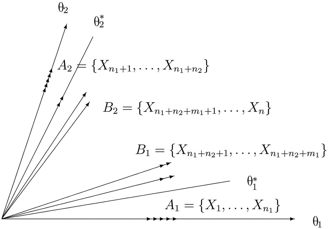
Theoretically, any coordinate system may be used in MIRT. To ensure that IRFs are monotone increasing (or nondecreasing) with respect to each ability, a constraint that all discrimination parameters are nonnegative is imposed on the MIRT models. Hence, a coordinate system has to be chosen such that all discrimination vectors lie in the first quadrant. As such, the coordinate axes are chosen to be the d directions of the most separated items in this article so that other items are in the first quadrant as shown in Figure 1, when d = 2. Here, the discrimination vector of an item is used to represent the item in the latent space. In practice, the coordinate axes are usually the target abilities that a test measures. For convenience, these coordinate axes are called the target subscales in this article. Note that these coordinate axes are oblique in the sense that they (e.g., algebra and geometry) are usually positively correlated. When speaking of content-specific or comprehensive items (i.e., items measuring one subscale or more than one subscale), this article always refers to this coordinate system.

Figure 1.

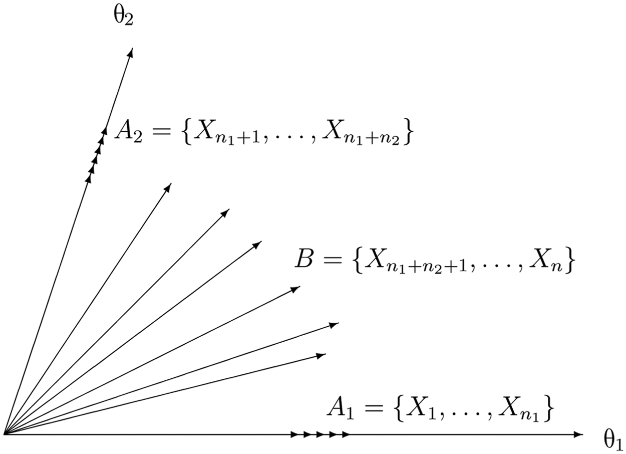
A two-dimensional test with mixed structure

Simple Structure

Let A = (a_ik) be the n × d discrimination matrix. The rank of A should be d, otherwise the dimensional structure of the test (with its fixed examinee population) is degenerate (see Zhang, 1996). One special degenerate case is the unidimensional case, which occurs when the rank of A is one. In this case, every discrimination vector is in the same direction (see Reckase, Ackerman, & Carlson, 1988). When the rank of A is d, there exist d linear independent discrimination vectors such that other discrimination vectors are linear combinations of these d discrimination vectors. If every discrimination vector is in the same direction as one of these d discrimination vectors, then the test has a simple structure. In this case, after some rotation, every discrimination vector will have one and only one positive element, and all other elements will be zero; that is, each item loads on one theta axis only. In practice, it is often assumed that the number of dimensions in an assessment is the number of domains or strands to be measured, and each item measures one and only one domain. For example, suppose a mathematics test is well fitted with two latent variables, θ₁ and θ₂, representing two mathematics strands: algebra and geometry, respectively. Then, the IRF of an algebra item will be presumed to depend on θ₁ only, and it can be written as

P_{i_{1}} (θ_{1}, θ_{2}) \equiv P_{i_{1}} (θ_{1}) = c_{i_{1}} + (1 - c_{i_{1}}) \frac{1}{1 + exp {- 1.7 a_{i_{1} 1} (θ_{1} - b_{i_{1}})}},

for i₁ = 1, 2, …, n₁. It is a unidimensional 3PL or 2PL model when $c_{i_{1}} = 0$ (see Lord, 1980). Similarly, the IRF of a geometry item can be written as,

P_{i_{2}} (θ_{1}, θ_{2}) \equiv P_{i_{2}} (θ_{2}) = c_{i_{2}} + (1 - c_{i_{2}}) \frac{1}{1 + exp {- 1.7 a_{i_{2} 2} (θ_{2} - b_{i_{2}})}},

for i₂ = n₁ + 1, n₁ + 2, …, n. That is, $a_{i_{1} 2} \equiv 0$ for all algebra items and $a_{i_{2} 1} \equiv 0$ for all geometry items. In other words, each content-based subtest is assumed to be unidimensional in an SST. Hence, a unidimensional calibration program, such as BILOG, can be applied to each subtest to estimate item parameters.

Clearly, an SST is a special case of a multidimensional test as Equations 2 and 3 are special cases of the larger model (Equation 1) under the constraint that one, and only one, of a_ik, k = 1, …, d, is positive. A multidimensional calibration program can also be applied to estimate item parameters for all items simultaneously under the constraint that each item measures only one domain.

Maximum likelihood estimation (MLE) is the most popular method used to estimate unknown parameters. In IRT, the item parameters are the structural parameters and the ability parameters are the incidental parameters (Hambleton & Swaminathan, 1985). Depending on how one treats the incidental parameters, there are two popular methods in IRT to estimate parameters: the JMLE and MMLE methods. The major difference between the JMLE and the MMLE is the treatment of abilities. In the JMLE method, abilities are treated as fixed unknown parameters, whereas in the MMLE method, abilities are treated as random variables with a prior distribution. In the following, the unidimensional and multidimensional approaches are compared for an SST when the JMLE or the MMLE method is used to estimate item parameters.

JMLE

Let x₁, x₂, …, x_N be the response vectors from N randomly sampled examinees with abilities θ₁, θ₂, …, θ_N. By the local independence assumption, the joint probability of a particular response pattern x_j = (x_j1, …, x_jn) across a set of n items given the jth examinee’s θ_j is

P (x_{j} | θ_{j}, Γ) = \prod_{i = 1}^{n} P_{i} {(θ_{j})}^{x_{j i}} {(1 - P_{i} (θ_{j}))}^{1 - x_{j i}}, j = 1, 2, \dots, N,

where P_i(θ) is the IRF, N is the number of examinees, and Γ represents all item parameters in the test. Denote

Θ = (\begin{matrix} θ_{1} \\ θ_{2} \\ ⋮ \\ θ_{N} \end{matrix}) = (\begin{matrix} θ_{11} & θ_{12} & \dots & θ_{1 d} \\ θ_{21} & θ_{22} & \dots & θ_{2 d} \\ ⋮ & ⋮ & ⋮ & ⋮ \\ θ_{N 1} & θ_{N 2} & \dots & θ_{N d} \end{matrix}) .

θ is the N × d ability score matrix, and $θ = (θ_{1}, θ_{2}, \dots, θ_{d})$ , where $θ_{k} = (θ_{1 k}, θ_{2 k}, \dots, θ_{Nk})'$ is the ability vector of the kth dimension for the N examinees.

When the test is a d-dimensional SST, it consists of d subtests with n₁, n₂, …, n_d items, respectively. Here, n = n₁ + n₂ + … + n_d. The response vector of examinee j can be decomposed into d parts: x_j = (x_j1 + x_j2 + … + x_jd), where x_jk is the response vector of examinee j to subtest k for j =1, 2, …, N and k =1, 2, …, d. Here, x_j = (x_j1 + x_j2 + … + x_jd) and $x_{jk} = (x_{j (n_{1} + \dots + n_{k - 1} + 1)}, \dots, x_{j (n_{1} + \dots + n_{k})})$ for k = 2, …, d. Denote

X = (\begin{matrix} x_{1} \\ x_{2} \\ ⋮ \\ x_{N} \end{matrix}) = (\begin{matrix} x_{11} & x_{12} & \dots & x_{1 d} \\ x_{21} & x_{22} & \dots & x_{2 d} \\ ⋮ & ⋮ & ⋮ & ⋮ \\ x_{N 1} & x_{N 2} & \dots & x_{N d} \end{matrix}) .

X is the N × n response data matrix of the test. Let $X_{k} = (x'_{1 k}, x'_{2 k}, \dots, x'_{Nk})'$ be the N × n_k response data matrices of the kth subtest. Then, X = (X₁, X₂, …, X_k). Correspondingly, denote Γ = (Γ₁, Γ₂, …, Γ_d), where Γ_k represents all item parameters in subtest k.

As each item is only associated with one dimension, the joint probability (Equation 4) of the response vector x_j = (x_j1, x_j2, …, x_jd) given θ_j = (θ_j1, θ_j2, …, θ_jd) can be written as,

\begin{matrix} P (x_{j} | θ_{j}, Γ) \equiv P (x_{j 1}, x_{j 2}, \dots, x_{j d} | θ_{j 1}, θ_{j 2}, \dots, θ_{j d}, Γ_{1}, Γ_{2}, \dots, Γ_{j d}) \\ = \prod_{k = 1}^{d} \prod_{i_{k} = n_{1} + \dots + n_{k - 1} + 1}^{n_{1} + \dots + n_{k}} P_{i_{k}} {(θ_{j k})}^{x_{j i_{k}}} {(1 - P_{i_{1}} (θ_{j k}))}^{1 - x_{j i_{k}}} \\ = \prod_{k = 1}^{d} P (x_{j k} | θ_{j k}, Γ_{k}), \end{matrix}

where

P (x_{j k} | θ_{j k}, Γ_{k}) = \prod_{i_{k} = n_{1} + \dots + n_{k - 1} + 1}^{n_{1} + \dots + n_{k}} P_{i_{k}} {(θ_{j k})}^{x_{j i_{k}}} {(1 - P_{i_{1}} (θ_{j k}))}^{1 - x_{j i_{k}}}

are the joint probabilities of the kth subtest. Equation 5 shows that the joint probability of a response vector of a whole test with simple structure can be decomposed into the product of the joint probabilities of the d subtests.

Let L(θ, Γ; X) be the joint likelihood function of the response matrix X. Under the multidimensional approach, JMLE tries to find ${\hat{θ}}^{m}$ and ${\hat{Γ}}^{m}$ such that

L ({\hat{Θ}}^{m}, {\hat{Γ}}^{m}; X) = max_{Θ, Γ} L (Θ, Γ; X) .

${\hat{θ}}^{m}$ and ${\hat{Γ}}^{m}$ are the JMLEs of θ and Γ using the multidimensional approach. The “joint” comes from the fact that the item and ability parameters are simultaneously estimated.

Let L_k(θ_k, Γ_k; X_k) be the joint likelihood function of the response matrix of the kth subtest. Under the unidimensional approach, JMLE tries to separately find ( ${\hat{θ}}_{k}^{u}, {\hat{Γ}}_{k}^{u}$ ) such that

L_{k} ({\hat{Θ}}_{k}^{u}, {\hat{Γ}}_{k}^{u}; X_{k}) = \max_{Θ_{k}, Γ_{k}} L_{k} (Θ_{k}, Γ_{k}; X_{k}) .

From Equation 5, the joint likelihood function of the response patterns x₁, x₂, …, x_N from N randomly sampled examinees is

\begin{matrix} L (Θ, Γ; X) = \prod_{j = 1}^{N} P (x_{j} | θ_{j}, Γ) = \prod_{j = 1}^{N} \prod_{k = 1}^{d} P (x_{j k} | θ_{j k}, Γ_{k}) \\ = \prod_{k = 1}^{d} \prod_{j = 1}^{N} P (x_{j k} | θ_{j k}, Γ_{k}) = \prod_{k = 1}^{d} L_{k} (Θ_{k}, Γ_{k}; X_{k}) . \end{matrix}

Equation 7 shows that the joint likelihood function of a whole test with simple structure can be decomposed into the product of the joint likelihood functions of subtests. According to Equation 7, maximizing L(θ, Γ; X) over θ and Γ (i.e., the multidimensional approach) is equivalent to maximizing all L_k(θ_k, Γ_k; X_k) over θ_k and Γ_k for k = 1, …, d (i.e., the unidimensional approach). Hence, under the simple structure assumption, the unidimensional and multidimensional approaches will give the exact same parameter estimates, if both use JMLE to estimate parameters. The same result can also be found in Yao and Boughton (2007) and Zhang (2004).

However, JMLE estimates are not consistent. Lord (1986) found that JMLE obtains biased estimates of ability and item parameters in unidimensional cases when there are only 10 or 15 items, even when the number of examinees is large. JMLE will not be discussed any further in this article.

MMLE

The MMLE approach (Bock & Aitkin, 1981) is the most widely used method in IRT for the estimation of item parameters. BILOG and PARSCALE use this method. In the MMLE method, latent abilities are treated as random variables. The (prior) distribution of the latent ability vector is typically assumed to be a multivariate normal distribution. Without loss of generality, one can standardize the latent traits so that they have means of zero and variances of one.

For the multidimensional approach, the marginal likelihood function can be calculated as below. From Equation 5, the marginal probability of an observed response pattern x_j for a randomly sampled examinee j is

P (x_{j} | Σ, Γ) = \int_{- \infty}^{+ \infty} \dots \int_{- \infty}^{+ \infty} \prod_{k = 1}^{d} P (x_{j k} | θ_{j k}, Γ_{k}) φ (θ_{j 1}, \dots, θ_{j d} | Σ) d θ_{j 1} \dots d θ_{j d},

where φ(θ_j|Σ) ≡ φ(θ_1j, …, θ_dj|Σ) is the density function of the (standardized) ability vector and Σ being the d × d correlation matrix. The marginal likelihood function of the whole response data matrix X is given by

L (Σ, Γ; X) = \prod_{j = 1}^{N} P (x_{j} | Σ, Γ) .

Under the multidimensional approach, MMLE tries to find ${\hat{Σ}}^{m}$ and ${\hat{Γ}}^{m}$ such that

L ({\hat{Σ}}^{m}, {\hat{Γ}}^{m}; X) = \max_{Σ, Γ} L (Σ, Γ; X) .

For the unidimensional approach, the marginal probability of response pattern x_jk of the kth subtest is

P (x_{j k} | Γ_{k}) = \int_{- \infty}^{+ \infty} P (x_{j k} | θ_{j k}, Γ_{k}) φ (θ_{j k}) d θ_{j k} for k = 1, \dots, d,

where φ(θ_jk) is the marginal density function of the kth ability and is the standard normal density function if φ(θ_1j, …, θ_jd|Σ) is multivariate normal. The marginal likelihood functions given response data matrices X_k of the kth subtest is

L_{k} (Γ_{k}; X_{k}) = \prod_{j = 1}^{N} P (x_{j k} | Γ_{k}) for k = 1, \dots, d .

Under the unidimensional approach, MMLE tries to find ${\hat{Γ}}_{k}^{u}$ such that

L_{k} ({\hat{Γ}}_{k}^{u}; X_{k}) = \max_{Γ_{k}} L_{k} (Γ_{k}; X_{k}) for k = 1, \dots, d .

From Equations 8 and 10, in general,

P (x_{j} | Σ, Γ) \neq \prod_{k = 1}^{d} P (x_{j k} | Γ_{k}),

unless abilities (i.e., underlying dimensions) are uncorrelated (i.e., independent if abilities are multivariate normal); that is, Σ is a d × d identity matrix. Therefore, from Equations 9, 11, and 12, in general,

L (Σ, Γ; X) \neq \prod_{k = 1}^{d} L_{k} (Γ_{k}; X_{k}) .

Hence, the MMLE of Γ using the multidimensional approach, ${\hat{Γ}}^{m}$ , may be quite different from the MMLE of Γ using the unidimensional approach, ${\hat{Γ}}^{u} = ({\hat{Γ}}_{1}^{u}, \dots, {\hat{Γ}}_{d}^{u})$ , when Σ is not an identity matrix. In sum, under the unidimensional assumption, the MMLEs of item parameters using the multidimensional approach are different from those obtained from the unidimensional approach except when the correlation coefficients between underlying dimensions of simple structure are known to be zero.

The essential difference between the unidimensional and multidimensional approaches for an SST is how the population distribution of abilities is applied. The multidimensional approach uses the joint distribution of abilities and estimates the correlations at the same stage as when estimating item parameters, whereas the unidimensional approach only uses the marginal distributions of abilities and the correlations are typically estimated after estimating item parameters. For example, NAEP uses the unidimensional approach to estimate item parameters and then the plausible value methodology (Mislevy, 1991) to obtain the estimated correlation coefficients. It should be noted that the unidimensional approach regards the correlations between abilities as unknown; therefore, they need to be estimated at a later stage. Thus, the values of correlations between abilities do not have an effect on the estimation of item parameters when the unidimensional approach is applied. However, it does not mean that the unidimensional approach assumes that abilities are uncorrelated or independent.

The preceding result shows that two different sets of item parameter estimates will be obtained from the unidimensional and multidimensional approaches using the MMLE method for an SST. As the unidimensional approach is usually used in operational data analyses for an SST, it is of interest to know whether the multidimensional approach can improve the accuracy of item parameter estimates. To investigate which approach provides better recovery of item parameters, a simulation study is conducted in the following section.

A Simulation Study With Simple Structure

Simulated response data were used to compare the accuracy of item parameter estimates obtained from the unidimensional and multidimensional approaches when the MMLE method was applied. Many unidimensional and multidimensional estimation programs based on the MMLE method are available for use. Considering that the effect of different dimensional approaches on the accuracy of item parameter estimation may be confounded with the effect of other factors (such as differences in algorithms and differences in levels of numerical accuracy obtained from different computer programs), it is not appropriate to compare the two approaches using different estimation programs. For comparison purposes, one has to choose the same estimation program (software) that can estimate item parameters for unidimensional and multidimensional IRT models. In both simulation studies in this article, an estimation program, called ASSEST (Zhang, 2005), was selected to estimate item parameters.

ASSEST is designed to estimate item parameters for unidimensional and multidimensional IRT models with mixed structures. It adopts an expectation-maximization–genetic algorithm (EM-GA) to estimate item parameters using the MMLE method. The EM algorithm is an iterative method for finding maximum likelihood estimates of parameters for probability models (e.g., Bock & Aitkin, 1981). Each iteration consists of two steps: the E step (expectation) and the M step (maximization). The EM algorithm is applied to estimate the parameters for each item individually, and then the iteration process is repeated until certain convergence criteria are met (e.g., the changes of likelihood function values and all item parameter estimates are smaller than preselected values). The algorithm is called the EM-GA algorithm because a GA is used in the maximization step of the EM algorithm. A GA is a computational algorithm that takes ideas from genetics and/or evolution (e.g., breeding, mutation, crossover, and survival of the fittest) and can be used to solve any optimization problem, such as adaptive control, cognitive modeling, optimal control problems, and traveling salesman problems (Michalewicsz, 1994). A GA starts with a set of potential solutions (called individuals) to a problem at hand. Then it stochastically optimally selects individuals as parents of the next generation and lets the selected individuals clone, mutate, and combine some of their components to form new individuals (offspring). This process is repeated over successive generations until one cannot find another individual better than the optimal individual one has gotten thus far. By using a well-designed GA in the maximization step of the EM algorithm, the chance of obtaining the global maximum value is increased. For details about ASSEST, see Zhang (2005). As ASSEST uses the same algorithm to estimate unidimensional and multidimensional IRT models, it is appropriate to apply ASSEST to compare the unidimensional and multidimensional approaches without algorithm and numerical accuracy complications. When running ASSEST, one can choose the unidimensional approach by specifying each subtest as unidimensional and estimating its item parameters separately from other subtests, or choose the multidimensional approach by estimating item parameters of all subtests simultaneously.

Simulation Design

The test length in this simulation was set to be either 30, 46, or 62 items. The estimated item parameters of dichotomous items from the analysis of the 1998 NAEP Grade 4 reading assessment (see Appendix E of Allen et al., 2001) were used as “true” item parameters in these simulation studies. There are 31 dichotomous items measuring the first subscale of reading for literary experience, and 32 dichotomous items measuring the second subscale of reading to gain information. An item in the second subscale with b = 3.921 was dropped from these simulation studies. Therefore, there are a total of 62 items with 35 multiple-choice and 27 constructed-response items. A 3PL model is used for the multiple-choice items and a 2PL model for the constructed-response items. For completeness, these item parameters are given in Table 1. For tests with 30 or 46 items, the first 15 or 23 items from each subscale were chosen. For instance, the items in the 30-item test are Items 1 to 15 and Items 32 to 46 are shown in Table 1.

Table 1.

Item Parameters From 1998 NAEP Grade 4 Reading Assessment

Reading for literary experience				Reading to gain information
Item	a ₁	b	c	Item	a ₂	b	c
1	0.623	−0.872	0.000	32	0.269	−0.904	0.000
2	1.506	−0.495	0.215	33	0.941	0.401	0.264
3	0.920	1.008	0.000	34	0.793	0.642	0.247
4	0.607	0.712	0.251	35	1.032	0.507	0.248
5	1.052	1.009	0.000	36	1.172	0.645	0.000
6	1.288	0.554	0.190	37	0.533	−0.835	0.218
7	1.798	−0.899	0.248	38	0.877	−0.523	0.000
8	0.754	0.015	0.000	39	1.203	0.257	0.165
9	1.342	−0.457	0.175	40	0.761	−1.242	0.000
10	0.763	−0.284	0.000	41	1.104	−0.155	0.247
11	1.110	0.148	0.244	42	0.619	−1.113	0.000
12	1.025	0.107	0.000	43	1.154	0.645	0.000
13	1.228	0.259	0.247	44	1.464	0.774	0.138
14	0.647	−1.008	0.000	45	1.536	1.192	0.000
15	0.520	−1.425	0.000	46	0.597	1.341	0.000
16	0.951	−0.864	0.319	47	2.300	0.416	0.264
17	0.757	−0.630	0.000	48	0.562	−0.073	0.237
18	0.832	1.118	0.000	49	0.970	0.906	0.000
19	1.472	1.204	0.167	50	0.883	−1.015	0.310
20	1.859	0.213	0.265	51	1.261	1.084	0.206
21	1.123	1.057	0.000	52	0.597	−0.206	0.156
22	1.133	0.916	0.297	53	0.938	−1.691	0.294
23	1.374	0.307	0.269	54	1.086	−0.060	0.000
24	0.504	−0.932	0.247	55	0.795	−0.238	0.000
25	1.415	0.891	0.271	56	1.414	−0.608	0.275
26	2.303	0.609	0.418	57	0.838	−0.076	0.000
27	0.814	0.306	0.000	58	1.185	−0.590	0.312
28	0.966	−1.318	0.244	59	1.031	−0.310	0.000
29	0.506	−1.272	0.000	60	0.579	−0.688	0.276
30	1.029	0.327	0.300	61	0.970	−0.502	0.270
31	0.721	−1.193	0.247	62	1.002	−0.530	0.000

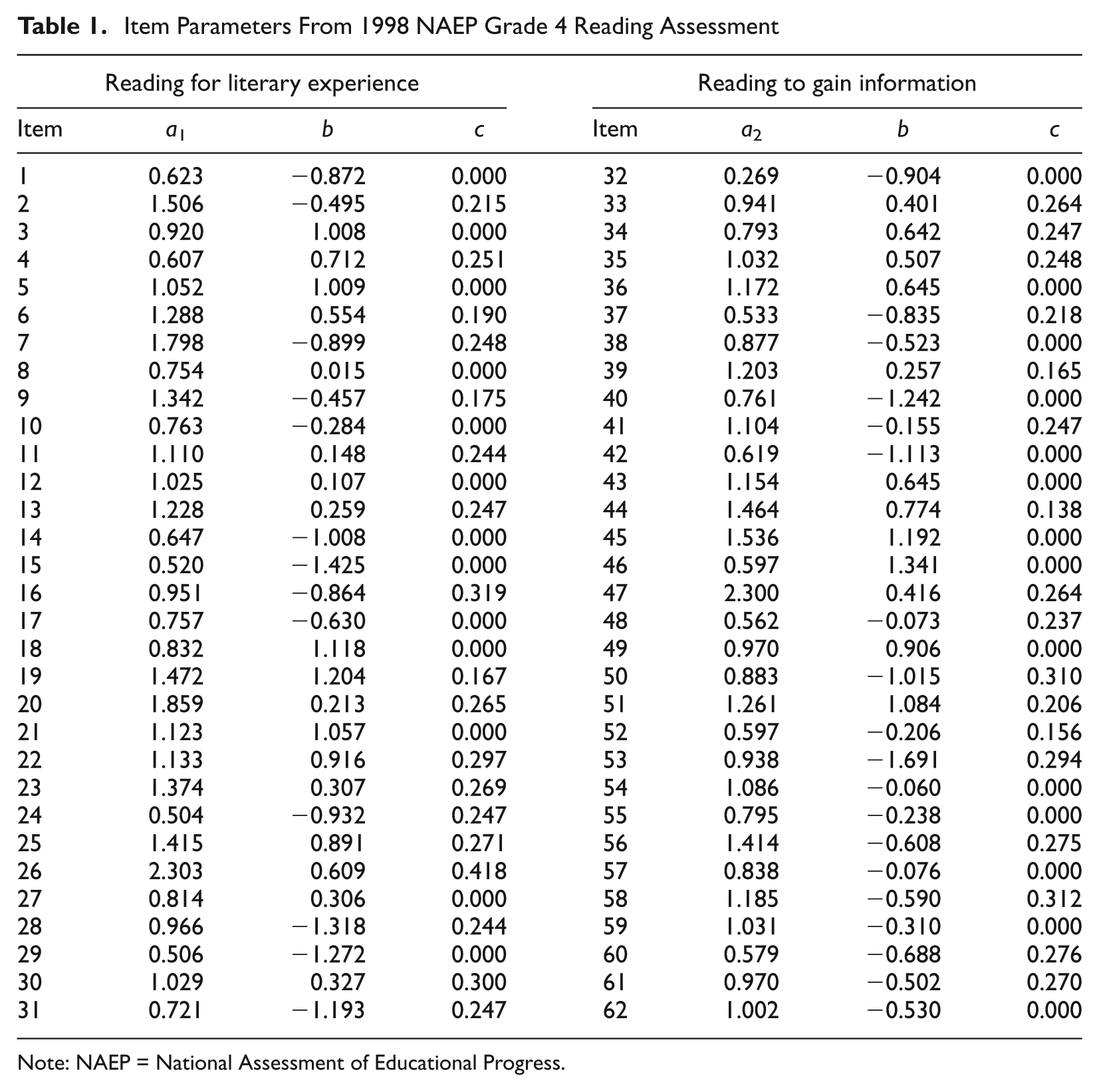
Note: NAEP = National Assessment of Educational Progress.

The number of simulated examinees was 500, 1,000, 2,000, 3,000, 4,000, or 5,000 in this study. Examinees’ (true) ability scores were generated independently from bivariate normal distributions with means of 0, variances of 1, and a (population) correlation of 0, .5, or .8. When the correlation coefficient is zero, theoretically, there should be no difference between the unidimensional and multidimensional approaches. Any difference between the unidimensional and multidimensional approaches when the correlation coefficient is zero is caused by numerical rounding error in the calibration program, which provides a reference when comparing differences in other cases. Of course, the multidimensional approach has additional errors from estimation of the correlation. However, the impact should be small, if not negligible, as the errors from estimation of the correlation are typically small.

Simulated response data were generated using the following (standard) IRT method. Given ability score θ_j, first calculate the probability of answering item i correctly by examinee j, p_ij = P_i(θ_j), using item parameters from Table 1. Then generate a random number r from the (0, 1) uniform distribution. If r < p_ij, then a correct response was obtained for examinee j on item i; otherwise, an incorrect response was obtained.

In summary, the following three factors were considered in this simulation study:

The number of items: 30, 46, or 62

The number of simulated examinees: 500, 1,000, 2,000, 3,000, 4,000, or 5,000

The correlation coefficient between two subscales: 0, .5, or .8

Given these factors, there were 54 combinations in this simulation. For each combination, ASSEST was applied to a simulated response data set twice to get two sets of parameter estimates under two different specifications, corresponding to the unidimensional and multidimensional approaches. This process was repeated 100 times for each combination.

Criterion for Comparisons

In this simulation study, two different kinds of root mean squared errors (RMSEs) were calculated as comparison criterions. The first kind focuses on the recovery of item parameters and the second kind on the direct recovery of IRFs.

The RMSE of estimated parameters is commonly used as a criterion for the recovery of item parameters in simulation studies. The RMSE is the square root of the average of the squared deviations of estimated parameters from the corresponding true ones. Let γ_i represent a parameter of item i, a_i1, a_i2, b_i, or c_i, and ${\hat{γ}}_{ij}$ be the estimate of γ_i from the jth replication for i = 1, …, n and j = 1, …, J. Here, n is the number of items and J is the number of replications (J = 100 in the simulation studies). For each item parameter, define

RMSE (γ_{i}) = \sqrt{\frac{1}{J} \sum_{j = 1}^{J} {({\hat{γ}}_{i j} - γ_{i})}^{2}} .

Given an SST with n items, the total number of item parameters is 2n (n discrimination and n difficulty parameters) plus the number of lower asymptote parameters (i.e., the number of items in the test modeled by the M3PL model). The number of RMSEs is the same as the number of item parameters. To make the comparison feasible, these RMSEs are further summarized by types of item parameters. If the test has two subtests, then there are four types of item parameters: the discrimination parameter for the first subscale a₁, the discrimination parameter for the second subscale a₂, the difficulty parameter b, and the lower asymptote parameter c for multiple-choice items. To further summarize the RMSE, the average of the RMSEs (ARMSE) for each of these four kinds of item parameters is defined as

ARMSE (γ) = \frac{1}{# S_{γ}} \sum_{i \in S_{γ}} RMSR (γ_{i}) = \frac{1}{# S_{γ}} \sum_{i \in S_{γ}} \sqrt{\frac{1}{J} \sum_{j = 1}^{J} {({\hat{γ}}_{i j} - γ_{i})}^{2}},

where γ represents one of the four kinds of item parameters, S_γ is the set of item sequence numbers that have γ parameter and #S_γ is the number of elements in S_γ. If γ is the discrimination parameter of the second subscale, for example, then S_a2 = {n₁ + 1, n₁ + 2, …, n} and #S_a2 = n₂. If γ is the lower asymptote parameter, then S_c = {i: item i is a multiple-choice item, 1 ≤i≤n} and #S_c is the number of items modeled by M3PL models. For each of the two different dimensional estimation approaches, there are four ARMSE(γ)s for each of the 54 combinations considered in the simulation study. These values (total of 2 × 4 × 54 = 432) together with ARMSE of estimated IRF defined later are reported in Table 2, which is discussed later.

Table 2.

ARMSE of Estimated Item Parameters and IRF When the Correlation Between Subscales Is 0 (Based on 100 Replications Using Unidimensional [U] and Multidimensional [M] Approaches)

		a ₁		a ₂		b		c		IRF
Number of examinees	Number of items	U	M	U	M	U	M	U	M	U	M
500	30	.231	.234	.234	.233	.185	.185	.098	.098	.032	.032
	46	.247	.247	.220	.220	.192	.192	.096	.097	.032	.032
	62	.246	.246	.211	.211	.192	.192	.101	.101	.030	.030
1,000	30	.159	.160	.155	.154	.139	.139	.077	.077	.023	.023
	46	.166	.164	.153	.154	.149	.150	.076	.077	.024	.024
	62	.170	.170	.150	.150	.150	.149	.083	.082	.022	.022
2,000	30	.112	.111	.105	.105	.105	.105	.058	.058	.017	.017
	46	.118	.117	.107	.108	.118	.118	.058	.059	.018	.018
	62	.124	.125	.108	.108	.115	.115	.064	.064	.016	.016
3,000	30	.095	.093	.088	.089	.092	.091	.049	.049	.015	.015
	46	.099	.098	.092	.092	.104	.105	.050	.050	.016	.016
	62	.105	.104	.092	.092	.101	.100	.055	.054	.014	.014
4,000	30	.085	.085	.076	.077	.083	.083	.044	.044	.013	.013
	46	.085	.084	.081	.081	.095	.095	.045	.045	.015	.015
	62	.092	.091	.083	.082	.091	.091	.049	.049	.012	.012
5,000	30	.074	.076	.068	.068	.077	.077	.040	.040	.012	.012
	46	.074	.073	.073	.072	.089	.088	.041	.041	.014	.014
	62	.083	.082	.076	.075	.086	.084	.046	.045	.011	.011

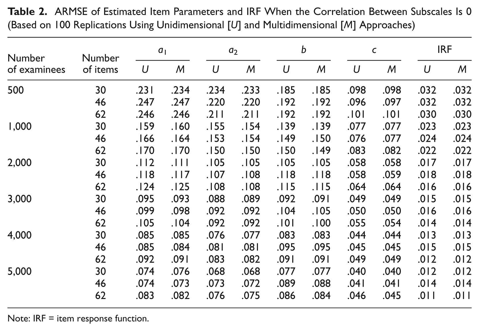
Note: IRF = item response function.

The estimates of item parameters are usually treated as fixed in any further analysis of response data such as estimating abilities of examinees. In the process of such analysis, the IRF is more directly relevant than item parameters themselves in operational applications as most statistical analysis is based on the likelihood function formed by the IRFs. In addition, different sets of item parameters may produce very similar item characteristic curves or surfaces. Therefore, it is more appropriate and vital to check the closeness of estimated IRF (curves or surfaces) to the true IRF than the item parameter estimates to the true values. Moreover, it is possible when making comparisons using the ARMSE of estimated parameters, one approach is better than the other for some parameters (e.g., discrimination parameters), but worse for other parameters (e.g., the lower asymptote parameter). This happened in the simulation study, for instance, in the cases of 62 items with .8 correlation (see the third part of Table 2). Hence, it is necessary to directly use the RMSE for the estimated IRF. Let ${\hat{P}}_{ij} (θ)$ be the estimated IRF of true IRF P_i(θ) from the jth replication. The RMSE of ${\hat{P}}_{ij} (θ)$ is defined as

d_{i j} = \sqrt{\int \dots \int {[{\hat{P}}_{i j} (θ) - P_{i} (θ)]}^{2} φ (θ | Σ) d θ_{1} \dots d θ_{d}},

where φ(θ|Σ) is the density function of the (standardized) latent ability vector and Σ is its correlation matrix. The RMSE of an estimated IRF is its Euclidean distance from its corresponding true IRF. Clearly, the smaller the RMSE, the better the estimator is.

The RMSEs of different IRFs in the same test may be quite different from each other because of different item characteristics. The average of the RMSEs among the items in a test across all replications will be used as an overall measure of the accuracy of the estimation, that is, the overall average $\bar{d} = 1 / nJ \sum_{i = 1}^{n} \sum_{j = 1}^{J} d_{ij}$ (called the ARMSE of estimated IRF). For each of the 54 combinations considered in this study, two ARMSEs were calculated based on the estimated IRF from the unidimensional and multidimensional approaches, respectively, and are reported in the last columns of Tables 2 to 4.

Table 3.

ARMSE of Estimated Item Parameters and IRF When the Correlation Between Subscales Is .5 (Based on 100 Replications Using Unidimensional [U] and Multidimensional [M] Approaches)

		a ₁		a ₂		b		c		IRF
Number of examinees	Number of items	U	M	U	M	U	M	U	M	U	M
500	30	.245	.247	.224	.218	.191	.187	.100	.098	.032	.032
	46	.253	.259	.224	.227	.195	.198	.095	.095	.032	.033
	62	.251	.260	.211	.217	.191	.191	.101	.100	.030	.030
1,000	30	.170	.169	.149	.148	.144	.140	.077	.076	.023	.023
	46	.172	.174	.151	.154	.150	.157	.075	.076	.024	.026
	62	.175	.181	.147	.153	.149	.150	.080	.081	.022	.022
2,000	30	.119	.121	.103	.104	.106	.102	.058	.056	.017	.017
	46	.122	.124	.108	.111	.117	.126	.059	.059	.019	.021
	62	.124	.131	.108	.114	.114	.115	.063	.063	.016	.017
3,000	30	.096	.095	.083	.083	.087	.086	.047	.048	.014	.014
	46	.096	.101	.091	.093	.102	.111	.049	.049	.016	.019
	62	.104	.110	.093	.098	.098	.100	.054	.054	.013	.014
4,000	30	.084	.086	.075	.073	.081	.076	.044	.042	.013	.012
	46	.084	.088	.080	.084	.093	.103	.044	.045	.015	.018
	62	.092	.097	.083	.087	.090	.091	.049	.048	.012	.013
5,000	30	.075	.075	.065	.067	.075	.072	.041	.039	.012	.011
	46	.076	.078	.072	.074	.088	.097	.041	.040	.014	.017
	62	.084	.087	.075	.079	.083	.085	.045	.044	.011	.012

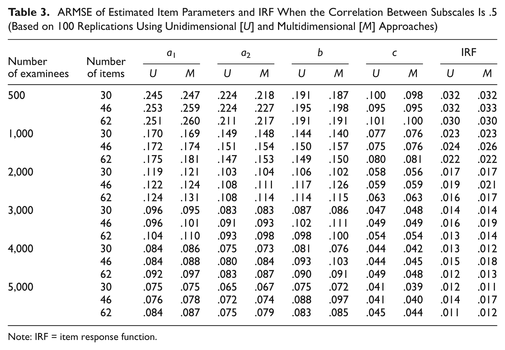
Note: IRF = item response function.

Table 4.

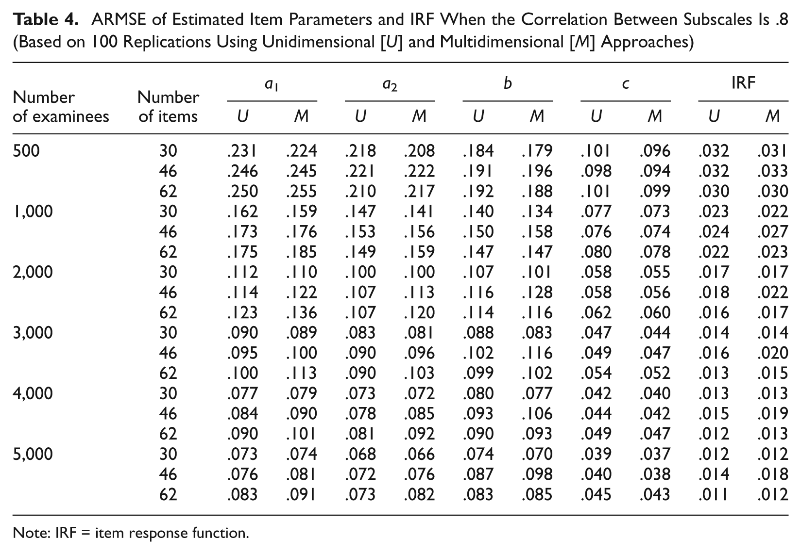
ARMSE of Estimated Item Parameters and IRF When the Correlation Between Subscales Is .8 (Based on 100 Replications Using Unidimensional [U] and Multidimensional [M] Approaches)

		a ₁		a ₂		b		c		IRF
Number of examinees	Number of items	U	M	U	M	U	M	U	M	U	M
500	30	.231	.224	.218	.208	.184	.179	.101	.096	.032	.031
	46	.246	.245	.221	.222	.191	.196	.098	.094	.032	.033
	62	.250	.255	.210	.217	.192	.188	.101	.099	.030	.030
1,000	30	.162	.159	.147	.141	.140	.134	.077	.073	.023	.022
	46	.173	.176	.153	.156	.150	.158	.076	.074	.024	.027
	62	.175	.185	.149	.159	.147	.147	.080	.078	.022	.023
2,000	30	.112	.110	.100	.100	.107	.101	.058	.055	.017	.017
	46	.114	.122	.107	.113	.116	.128	.058	.056	.018	.022
	62	.123	.136	.107	.120	.114	.116	.062	.060	.016	.017
3,000	30	.090	.089	.083	.081	.088	.083	.047	.044	.014	.014
	46	.095	.100	.090	.096	.102	.116	.049	.047	.016	.020
	62	.100	.113	.090	.103	.099	.102	.054	.052	.013	.015
4,000	30	.077	.079	.073	.072	.080	.077	.042	.040	.013	.013
	46	.084	.090	.078	.085	.093	.106	.044	.042	.015	.019
	62	.090	.101	.081	.092	.090	.093	.049	.047	.012	.013
5,000	30	.073	.074	.068	.066	.074	.070	.039	.037	.012	.012
	46	.076	.081	.072	.076	.087	.098	.040	.038	.014	.018
	62	.083	.091	.073	.082	.083	.085	.045	.043	.011	.012

Note: IRF = item response function.

Simulation Results

Tables 2 to 4 present the ARMSEs of the estimated item parameters and the estimated IRFs. Each table shows one of the three levels of correlation (0, .5, and .8, respectively). In columns 3 to 7, each cell has two numbers for the ARMSEs: The first comes from the unidimensional approach and the second from the multidimensional approach. Columns 3 to 6 are the ARMSEs for the discrimination parameter for the first subscale a₁, the discrimination parameter for the second subscale a₂, the difficulty parameter b, and the lower asymptote parameter c for multiple-choice items modeled by M3PL models. Note that the constructed-response items using 2PL models are not included in the calculation of RMSE of the lower asymptote parameter (see Equation 13). The last column in Tables 2 to 4 presents the ARMSE of the estimated IRFs. As expected, when the correlation between subscales and the number of items are fixed, the ARMSEs from both approaches decrease as the number of examinees increases. That is, the larger the number of examinees, the better the estimates from both approaches. Tables 2 to 4 show that when using the unidimensional approach, the ARMSEs are very close to each other when there are the same number of examinees and test length, regardless of which level of correlation between the subscales is used, which confirms that the correlation between subscales should have no impact on the performance of the unidimensional approach. Small differences may come from sampling variations across different levels of correlation. These tables also confirm that when the correlation between subscales is zero, these two approaches are basically the same. The slight difference of ARMSEs between these two approaches may come from the fact that in the multidimensional approach, the correlation coefficient is estimated, thereby causing an additional parameter to be estimated.

In most cases, the ARMSEs for the four kinds of item parameters give consistent results. However, in some cases, one approach yields smaller ARMSEs for some item parameters while yielding larger ARMSEs for other parameters (e.g., see Table 4). In such cases, the ARMSE of the IRFs is used as the final criterion. It is interesting to note that, in most cases, the multidimensional approach gives better estimates for the lower asymptote parameters.

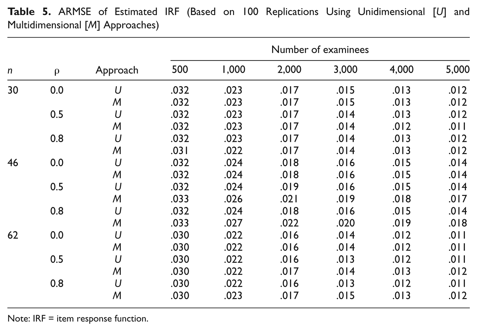
Tables 2 to 4 may be too large and complex to show the performance pattern of the two approaches clearly. The portions containing the ARMSEs for IRFs in these tables are reorganized and presented in Table 5, which shows that when the test length is 30 and the correlation is either .5 or .8, the average of the ARMSEs from the multidimensional approach is uniformly smaller than the corresponding average of the ARMSEs from the unidimensional approach across all numbers of examinees considered here. In contrast, when the test length is increased to 46 or 62, although the correlation still remains .5 or .8, the unidimensional approach is uniformly better (with smaller ARMSEs) than the multidimensional approach across all numbers of examinees. These results suggest that when the test length is relatively short, the additional information from other subscales’ items is helpful in obtaining more accurate IRF estimates if these scales are positively correlated. Otherwise, the additional information from other subscales may not be as helpful, and may even be harmful to the accuracy of parameter/IRF estimation, as additional statistical and numerical noises are also likely to be introduced when employing the multidimensional approach.

Table 5.

ARMSE of Estimated IRF (Based on 100 Replications Using Unidimensional [U] and Multidimensional [M] Approaches)

			Number of examinees
n	ρ	Approach	500	1,000	2,000	3,000	4,000	5,000
30	0.0	U	.032	.023	.017	.015	.013	.012
		M	.032	.023	.017	.015	.013	.012
	0.5	U	.032	.023	.017	.014	.013	.012
		M	.032	.023	.017	.014	.012	.011
	0.8	U	.032	.023	.017	.014	.013	.012
		M	.031	.022	.017	.014	.013	.012
46	0.0	U	.032	.024	.018	.016	.015	.014
		M	.032	.024	.018	.016	.015	.014
	0.5	U	.032	.024	.019	.016	.015	.014
		M	.033	.026	.021	.019	.018	.017
	0.8	U	.032	.024	.018	.016	.015	.014
		M	.033	.027	.022	.020	.019	.018
62	0.0	U	.030	.022	.016	.014	.012	.011
		M	.030	.022	.016	.014	.012	.011
	0.5	U	.030	.022	.016	.013	.012	.011
		M	.030	.022	.017	.014	.013	.012
	0.8	U	.030	.022	.016	.013	.012	.011
		M	.030	.023	.017	.015	.013	.012

Note: IRF = item response function.

Tables 2 to 5 only display the overall performance of the unidimensional and multidimensional approaches. To show results at the item level, this article introduces the percentage of counts where the multidimensional approach is better than the unidimensional approach based on the RMSE of the estimated IRF. Let

ξ = \sum_{i = 1}^{n} \sum_{j = 1}^{100} I (d_{i j}^{(m)} < d_{i j}^{(u)}),

where $d_{ij}^{(m)}$ and $d_{ij}^{(u)}$ are the RMSEs of IRF (Equation 14) from the multidimensional and unidimensional approaches, respectively, and I(A) is an indicator function that takes on the value of one if A is true and zero otherwise. The ξ counts the cases among all items and all replications that the RMSE of an estimated IRF from the multidimensional approach is smaller than that from the unidimensional approach (cases where the multidimensional approach is better than the unidimensional approach). Table 6 presents the results of these counts. The unidimensional approach is better in the cases where the percentages are less than 50%, whereas the multidimensional approach is better if the percentages are larger than 50%. Although the unidimensional approach is better when the test length is long and the multidimensional approach is better in the cases of relatively short test length, no one approach overwhelms the other in any of the 54 situations considered in this study. The largest percentage in Table 6 is 57.7%, where the test length is 30, the number of examinees is 500, and the correlation is .5, whereas the smallest percentage is 15.7% with 46 items, 5,000 examinees, and .8 correlation. Overall, in the 54 cases considered here, the unidimensional approach slightly outperforms the multidimensional approach. Note that the results in Table 6 depend on individual item characteristics and thus any comparison should only be made among the cases where the number of items is the same.

Table 6.

Percentage of Cases Where RMSE of Estimated IRF From Multidimensional Approach Is Smaller Than Unidimensional Approach (Comparing Each Items in Each Replication)

		Number of examinees
n	ρ	500	1,000	2,000	3,000	4,000	5,000
30	0.0	48.5	49.4	49.0	50.7	47.2	47.9
	0.5	55.8	55.7	55.3	55.4	56.3	56.3
	0.8	57.7	57.1	57.4	54.8	53.5	55.9
46	0.0	50.0	49.2	46.7	48.7	48.8	54.2
	0.5	38.6	32.2	23.0	22.2	19.7	18.9
	0.8	38.7	29.7	20.5	16.6	15.9	15.7
62	0.0	49.7	50.6	48.9	50.9	51.4	52.5
	0.5	45.7	42.6	40.0	40.2	41.3	41.4
	0.8	45.3	39.7	33.7	32.5	32.1	33.8

Note: RMSE = root mean squared error; IRF = item response function.

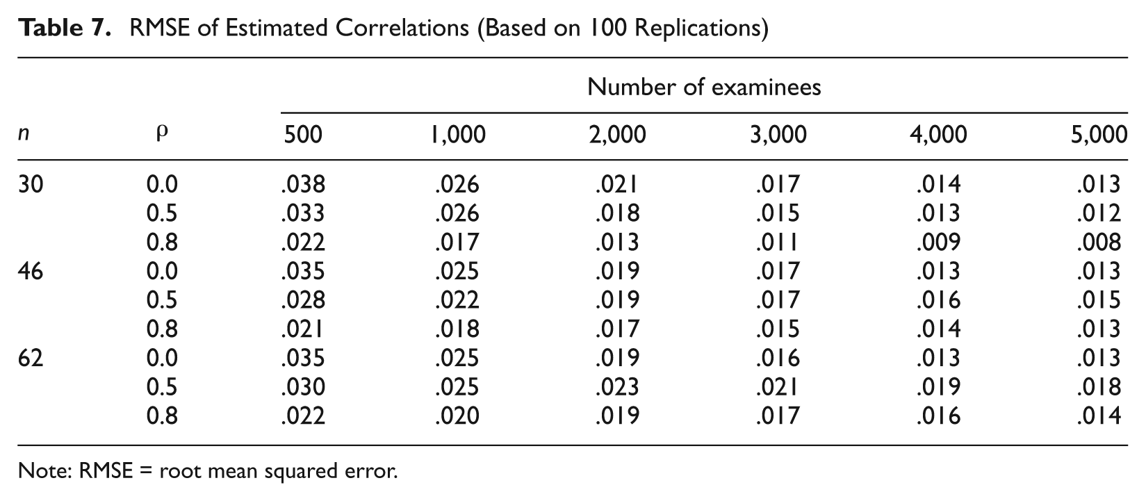
When using the multidimensional approach, the estimates of correlation coefficients between abilities are also obtained as a by-product. These estimates are relatively close to their corresponding true correlations. Table 7 presents the RMSEs of estimated correlations. As shown in Table 7, the largest RMSE is .038, which appears in the 30-item, 500-examinee, 0-correlation case, whereas the smallest RMSE is .008 in the 30-item, 5,000-examinee, .8-correlation case. Generally speaking, the greater the number of examinees, the better the estimated correlation is. However, the impact of test length and the correlation between subscales on the estimation of the correlation is not so straightforward. It seems that some interactions exist among these three factors. For example, when the test length is 30, for any fixed number of examinees, the RMSE decreases as the correlation increases. But when the number of items is 62, this pattern holds only in the case of 500 examinees (see Table 7). In uncorrelated cases (ρ = 0), with any fixed number of examinees, the RMSE decreases as the number of items increases. In contrast, when the correlation is either .5 or .8, the RMSE increases as the number of items increases except for the cases of 500 (with ρ = .5 or .8) or 1,000 (with ρ = .5 only) examinees as shown in Table 7. Note that in practice, subscales to be measured by a test are usually highly correlated. The cases of correlation between subscales being .5 or .8 are more important than uncorrelated cases. Focusing on the cases of correlation being .8, to get the same level of accuracy as in the 30-item case, more examinees were needed in the 62-item case. For instance, to achieve the same level of accuracy in the case of 30 items with 1,000 examinees, 3,000 examinees are needed in the case of 62 items.

Table 7.

RMSE of Estimated Correlations (Based on 100 Replications)

		Number of examinees
n	ρ	500	1,000	2,000	3,000	4,000	5,000
30	0.0	.038	.026	.021	.017	.014	.013
	0.5	.033	.026	.018	.015	.013	.012
	0.8	.022	.017	.013	.011	.009	.008
46	0.0	.035	.025	.019	.017	.013	.013
	0.5	.028	.022	.019	.017	.016	.015
	0.8	.021	.018	.017	.015	.014	.013
62	0.0	.035	.025	.019	.016	.013	.013
	0.5	.030	.025	.023	.021	.019	.018
	0.8	.022	.020	.019	.017	.016	.014

Note: RMSE = root mean squared error.

Mixed Structure

Simple structure requires that each item measures only one subscale. However, some items may turn out to measure several subscales although the test is designed to have simple structure. A test may require that some of its items measure more than one subscale according to its framework (see National Assessment Governing Board, 1994). Suppose a test is designed to measure d (d > 1) distinct subscales, A_k is the subset of items measuring subscale k only, and B is the subset of all comprehensive items measuring more than one subscale. This test is called a d-dimensional mixed structure test (MST). Figure 1 presents an example of a two-dimensional test with a mixed structure. When B is empty (i.e., there are no comprehensive items), the MST becomes an SST.

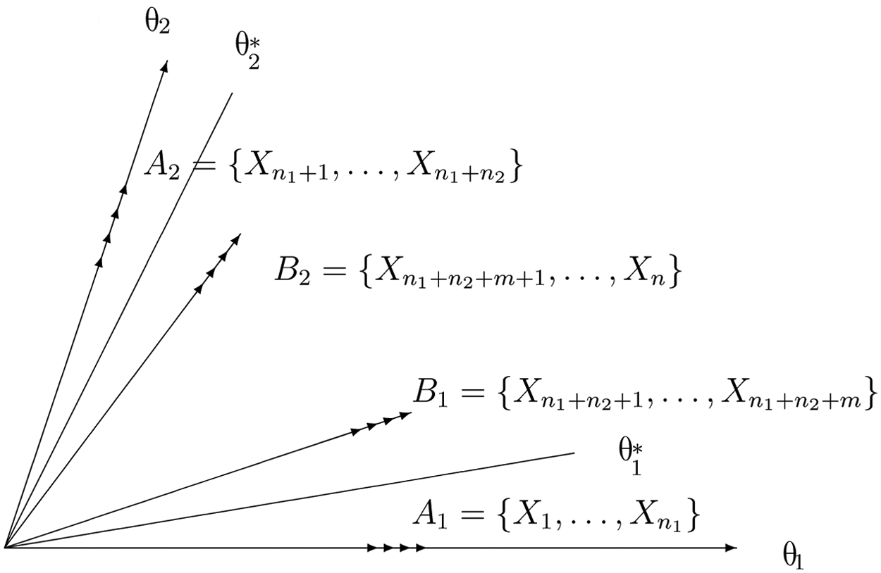
As mentioned earlier, even when the test framework requires that each item measure one subscale, some items may actually be “contaminated” in the sense that knowledge measured by the other subscales is helpful for an examinee to get correct answers for these items. Such an item usually has its target subscale as its dominant dimension although it is a comprehensive item. Such a test is called an approximate simple structure test (ASST), which consists of several subtests and each subtest is essentially unidimensional or has only one dominant distinct dimension. Clearly, approximate simple structure can be regarded as a special case of mixed structure when every comprehensive item has one of the subscales as its dominant dimension (or when no item measures two or more subscales equally well). When every subtest of an ASST is unidimensional, the ASST is an SST. A response data set with approximate simple structure is often treated as an SST in its statistical analysis, especially when the test is designed to be an SST. In the following, the author investigates the impact when an ASST is incorrectly specified as an SST in calibration.

As shown in Figure 2, there are two kinds of comprehensive items in a two-dimensional ASST: items in B₁ that mainly measure θ₁ and items in B₂ that mainly measure θ₂. For a d-dimensional ASST, the set of comprehensive items, B, can be decomposed into d subsets B_k for k = 1, …, d, where B_k is the subset of comprehensive items that mainly measure subscale k. Clearly, $B = \cup_{k = 1}^{B_{k}}$ .

Figure 2.

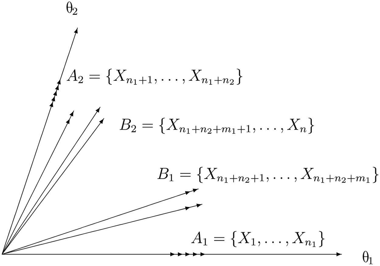
A two-dimensional test with approximate simple structure

Usually, it is not difficult to identify the optimal partition of items into d subtests S_k = A_k ∪ B_k, k = 1, …, d, from a dimensionality analysis when the sample size is moderately large. If S_k is calibrated as unidimensional, the subscale actually calibrated is $θ_{k}^{*}$ , a composite of the original d subscales as graphically shown in Figure 3 in the case of d = 2. The $θ_{k}^{*}$ is the composite best measured by subtest S_k and may be regarded as the reference composite of S_k (Wang, 1987). In reality, the reference composite may depend on the calibration method. In general,

θ_{k}^{*} = c_{k} (\sum_{l = 1}^{d} α_{k l} θ_{l}),

where α_kl (l =1, …, d) are the (unnormalized) weights that need to be determined, and c_k is the normalization factor so that $θ_{k}^{*}$ is standardized. After some calculation, one can obtain the correlation coefficients between the calibrated subscales as

ρ_{k_{1} k_{2}}^{*} = \frac{α_{k_{1}} Σ α_{k_{2}}^{'}}{\sqrt{α_{k_{1}} Σ α_{k_{1}}^{'}} \sqrt{α_{k_{2}} Σ α_{k_{2}}^{'}}} for 1 \leq k_{1}, k_{2} \leq d,

where α_k = (α_k1, …, α_kd) is the weight vector and Σ is the correlation matrix of the target subscales.

Figure 3.

The subscales calibrated are actually $θ_{1}^{*}$ and $θ_{2}^{*}$ when an ASST is incorrectly treated as an SST

Equation 16 gives the relationship between the correlation coefficients of the target subscales and the correlation coefficients of the calibrated subscales. Zhang and Stout (1999) theoretically defined a reference as the composite at which the expected multidimensional critical ratio function achieves its maximum value. According to Theorem 3 of Zhang and Stout (1999), the weights of the composite are mainly determined by the discrimination parameters. For subtest k (1 ≤ k ≤ d), an approximate formula of weights is

α_{k l} = \sum_{i \in S_{k}} a_{i l}, l = 1, \dots, d .

Specifically,

α_{k k} = \sum_{i \in A_{k}} a_{i k} + \sum_{i \in B_{k}} a_{i k} and α_{k l} = \sum_{i \in B_{k}} a_{i l} for l \neq k .

As B_k is the subset of items that mainly measure subscale k, a_ik > a_il (l ≠ k) for all items in B_k. Hence, for any fixed k, α_kk is always the largest weight among α_kl, l = 1, …, d}. In fact, {α_kk is usually much larger than the others. Thus, the $θ_{k}^{*}$ in Equation 15 is much closer to θ_k than the other θ_l for l ≠ k. Generally, all $θ_{k}^{*} s$ should lie inside the convex region spanned by θ_k, k =1, …, d, as all weights are nonnegative. Hence, the correlation coefficients between $θ_{k}^{*} s$ are larger than the corresponding correlation coefficients between θ_ks. Consequently, the correlation coefficients between the target subscales will be overestimated as the correlation coefficients between $θ_{k}^{*} s$ are actually estimated. The preceding results are summarized in the an theorem following.

Theorem

If an ASST is treated as an SST, the actual calibrated subscales are no longer the target subscales, although they could still be close to each other. The deviation of a calibrated subscale from its corresponding target subscale depends on how much the subtest departs from unidimensionality with the target subscale. The correlation coefficients between calibrated subscales given in Equation 16 are larger than those between their respective target subscales.

The theorem shows that when an ASST or an MST is incorrectly treated as an SST (i.e., MIRT models are misspecified), the calibrated subscales are no longer the target subscales and the correlation coefficients of the latent traits will be overestimated. From Equations 16 and 17, one may approximately calculate the expected correlation coefficients between the calibrated subscales. Next, a hypothetical example is used to illustrate how large the difference is between the calibrated subscales’ correlation and the target subscales’ correlation.

Example 1

Suppose that all items in B₁ measure the composite θ₁ + (2/3)θ₂ in the sense that the discrimination parameters of their secondary dimension (e.g., a_i2) equal two thirds of the discrimination parameters of their dominant dimension (e.g., a_i1), and all items in B₂ measure the composite (2/3)θ₁ + θ₂ as shown in Figure 4. If the magnitude of discrimination parameters and the numbers of items in all subsets are balanced, then according to Equation 15, $θ_{1}^{*}$ should be in the middle of A₁ (i.e., θ₁) and B₁ (i.e., θ₁ + (2/3)θ₂), and $θ_{2}^{*}$ in the middle of A₂ (i.e., θ₂) and B₂ (i.e., (2/3)θ₁ + θ₂); that is,

θ_{1}^{*} = c_{1} (θ_{1} + \frac{1}{3} θ_{2}), and θ_{2}^{*} = c_{2} (\frac{1}{3} θ_{1} + θ_{2}),

where c₁ and c₂ are the normalization constants. Let ρ be the correlation coefficient between the original two subscales, θ₁ and θ₂. Then, the correlation coefficient between $θ_{1}^{*}$ and $θ_{2}^{*}$ is

ρ^{*} = \frac{6 + 10 ρ}{10 + 6 ρ} .

Figure 4.

The correlation between the calibrated subscales $θ_{1}^{*}$ and $θ_{2}^{*}$ is (6 + 10ρ)/(10 + 6ρ) (e.g., .81), whereas the correlation between the target subscales θ₁ and θ₂ is ρ (e.g., .4) if the ASST is incorrectly treated as an SST

If the correlation between θ₁ and θ₂ is 0, .2, .4, .6, or .8, then the corresponding correlation between $θ_{1}^{*}$ and $θ_{2}^{*}$ is .60, .71, .81, .88, or .95, respectively.

A Simulation Study With Mixed Structure

To explore the consequences of the violation of simple structure, a second simulation study was conducted for an MST. Here, only the cases of 30 items with 1,000, 3,000, or 5,000 examinees with correlation .8 are reported.

To get an MST, the original two-dimensional SST was modified by changing some content-specific items into comprehensive items. Recall that each item in an SST has one and only one nonzero discrimination parameter (i.e., only one loading). By giving some positive value as its other discrimination parameter, a content-specific item becomes a comprehensive one. In this study, the first five items from each subscale (i.e., Items 1-5 and 32-36 in Table 1) were selected to become comprehensive items (measuring both subscales) by assigning two thirds of their existing discrimination parameter as their other discrimination parameter so that these modified items would still mainly measure their originally measured subscale. For example, the new second discrimination parameter was set to be 0.415 (i.e., 0:623 × 2/3) for the first item in Table 1. Consequently, the new 30-item test had 20 content-specific items (10 first-subscale items and 10 second-subscale items) and 10 comprehensive items (5 first-subscale dominated items and 5 second-subscale dominated items). This new set of item parameters and the originally generated ability scores with a population correlation of .8 from the simulation study in the section “A Simulation Study With Simple Structure” were used to generate new simulated item response data.

ASSEST was applied to each set of the simulated response data with two different specifications: First, the simulated response data set was incorrectly specified as two dimensional with simple structure, and second, the data set was correctly identified as two dimensional with mixed structure. In the former, the unidimensional and multidimensional approaches can be applied as before. The results from the unidimensional approach are not reported here as they are similar to the results from the multidimensional approach. In the latter case, only the multidimensional approach can be applied. The whole process was replicated 100 times, and the results are summarized in columns 2 and 3 of Table 8.

Table 8.

Summary Results for a 30-Item Test With 10 Modified Items and .8 Correlation (Based on 100 Replications Using Multidimensional Approach)

	ASST calibrated as an SST	ASST calibrated as an MST
Number of examinees = 1,000
ARMSE of estimated IRF (SD)	.041 (.002)	.026 (.003)
Average estimated correlation (SD)	.906 (.010)	.807 (.022)
RMSE of estimated correlation	.107	.021
Number of examinees = 3,000
ARMSE of estimated IRF (SD)	.035 (.002)	.018 (.002)
Average estimated correlation (SD)	.905 (.006)	.806 (.013)
RMSE of estimated correlation	.107	.014
Number of examinees = 5,000
ARMSE of estimated IRF (SD)	.034 (.001)	.016 (.003)
Average estimated correlation (SD)	.906 (.005)	.806 (.010)
RMSE of estimated correlation	.107	.011

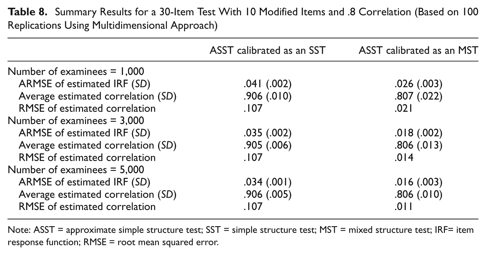
Note: ASST = approximate simple structure test; SST = simple structure test; MST = mixed structure test; IRF= item response function; RMSE = root mean squared error.

Table 8 shows that when the 10 modified items were incorrectly regarded as content-specific items (i.e., each data set was treated as though it had simple structure), the ARMSE of the estimated IRFs and the RMSE of the estimated correlation were relatively large (see column 2). When the 10 modified items were correctly treated as comprehensive items, the ARMSE of the estimated IRF and the RMSE of the estimated correlation were dramatically reduced (see column 3). For instance, the ARMSE of the estimated IRFs is .026 for 1,000 examinees compared with .041 when the modified items were incorrectly treated as content-specific items. The RMSE of estimated correlation is .021 in the case of 1,000 examinees whereas its counterpart is .107 in the mistreated case.

As shown in Table 8, the average estimated correlation between subscales when the test was misspecified as an SST is more than .9, whereas the true correlation is .8, which indicates the correlation was overestimated. If the test was correctly specified, the average of estimated correlations is between .806 and .807, and the RMSE is much smaller than that when the test was misspecified. When the 10 comprehensive items were incorrectly specified as content-specific items, one actually calibrated two composites, which were the combinations of the target subscales, as discussed in the preceding section. These two composites leaned closer to each other than the target subscales did. Not surprisingly, the correlation between target subscales was overestimated. From Equation 17, one may calculate the weights of the two calibrated subscales in the case here, α₁₁ = 15.183, α₁₂ = 3.139, α₂₁ = 2.805, and α₂₂ = 14.055. Hence, from Equation 16, the expected value of the correlation between the calibrated composites is approximately .907. When the models are incorrectly specified and the number of examinees is 5,000, the average estimated correlation is .906 (see column 2 of Table 8), which is very close to this expected value.

In sum, simulation results and the theorem in the section “Mixed Structure” demonstrate that it is not appropriate to treat an ASST or MST as an SST. One must examine the simple structure assumption before proceeding statistical analyses based on the assumption.

Discussion

In typical IRT applications, the estimated item parameters are treated as fixed in subsequent analyses of response data after item parameter estimation. Therefore, the accuracy of item parameter estimates plays an important role in the analyses. Under the simple structure assumption, the unidimensional and multidimensional approaches can be used to estimate item parameters. These two approaches are theoretically equivalent to each other if the JMLE method is used to estimate item parameters. However, when the MMLE method is applied, the estimates of item parameters obtained from these two approaches are different. A simulation study was conducted to further compare the unidimensional and multidimensional approaches with the MMLE method. The simulation results reveal that when the number of items is small, the multidimensional approach provides relatively more accurate estimates of item parameters; otherwise, the unidimensional approach prevails. Thus, when a test (e.g., NAEP) has enough items (say, 20) for each subscale, the unidimensional approach is better as long as the simple structure assumption is tenable.

The simple structure assumption is widely used in statistical analyses of response data from tests with multiple domains. Although it is less stringent than the unidimensionality assumption for the whole response data, the simple structure assumption is still a strong assumption. In many cases, it can be expected that this assumption will be violated. The results in the sections “Mixed Structure” and “A Simulation Study With Mixed Structure” demonstrate that inaccurate estimation results may be obtained if an MST is incorrectly specified as an SST. The simple structure assumption should be verified before doing any statistical analysis based on it. When a test does not have a simple structure, the multidimensional approach with an appropriate specification is recommended.

It should be noted that the unidimensional approach discussed in this article has a different focus than the unidimensional approximation approach which applies unidimensional models to multidimensional item response data (see Ackerman, 1989, 1994; Kahraman & Kamata, 2004; Reckase, Carlson, Ackerman, & Spray, 1986; Walker & Beretvas, 2003; Wang, 1988). The former applies unidimensional models to each unidimensional subtest, and the latter tries to approximate a whole test with unidimensional models. When the simple structure assumption does not hold, the unidimensional approach deals with the same problem as the unidimensional approximation approach does with each subtest.

Footnotes

Acknowledgements

The author would like to thank Ting Lu, Sarah Zhang, and two anonymous reviewers for their comments and suggestions.

Declaration of Conflicting Interests

The author(s) declared no potential conflicts of interest with respect to the research, authorship, and/or publication of this article.

Funding

The author(s) received no financial support for the research, authorship, and/or publication of this article.

References

Ackerman

T. A.

(1989). Unidimensional IRT calibration of compensatory and noncompensatory multidimensional items. Applied Psychological Measurement, 13, 113-127.

Ackerman

T. A.

(1994). Using multidimensional item response theory to understand what items and tests are measuring. Applied Measurement in Education, 20, 309-310.

Allen

Carlson

J. E.

Zelenak

(1999). The NAEP 1996 technical report (NCES 1999-452). Washington, DC: Office of Educational Research and Improvement, U.S. Department of Education.

Allen

Donoghue

J. R.

Schoeps

T. L.

(2001). The NAEP 1998 technical report (NCES 2001-509). Washington, DC: Office of Educational Research and Improvement, U.S. Department of Education.

Bock

R. D.

Aitkin

(1981). Marginal maximum likelihood estimation of item parameters: Application of the EM algorithm. Psychometrika, 46, 443-459.

Bradlow

E. T.

Wainer

Wang

(1999). A Bayesian random effects model for testlets. Psychometrika, 64, 153-168.

Cai

(2010a). High-dimensional exploratory item factor analysis by a Metropolis-Hastings Robbins-Monro algorithm. Psychometrika, 7, 33-57.

Cai

(2010b). A two-tier full-information item factor analysis model with applications. Psychometrika, 7, 581-612.

Cai

du Toit

S. H. C.

Thissen

(2009). IRTPRO: Flexible, multidimensional, multiple categorical IRT modeling [Computer software]. Chicago, IL: Scientific Software International.

10.

Fraser

(1988). NOHARM: A computer program for fitting both unidimensional and multidimensional normal ogive models of latent traits theory [Computer software]. Armidale, Australia: University of New England.

11.

Fraser

McDonald

R. P.

(1988). NOHARM: Least squares item factor analysis. Multivariate Behavioral Research, 23, 267-269.

12.

Hambleton

R. K.

Swaminathan

(1985). Item response theory: Principles and applications. Boston, MA: Kluwer-Nijhoff.

13.

Kahraman

Kamata

(2004). Increasing the precision of subscale scores by using out-of-scale information. Applied Psychological Measurement, 28, 407-426.

14.

Lord

F. M.

(1980). Applications of item response theory to practical testing problems. Hillsdale, NJ: Lawrence Erlbaum.

15.

Lord

F. M.

(1986). Maximum likelihood and Bayesian parameter estimation in item response theory. Journal of Educational Measurement, 23, 157-162.

16.

Michalewicsz

(1994). Genetic algorithms + data structures = genetic programs. Berlin, Germany: Springer-Verlag.

17.

Miller

T. R.

(1991). Empirical estimation of standard errors of compensatory MIRT model parameters obtained from the NOHARM estimation program (Research Report ONR 91-2). Iowa City, IA: American College Testing.

18.

Mislevy

(1991). Randomization-based inference about latent variables from complex samples. Psychometrika, 56, 177-196.

19.

Mislevy

Bock

R. D.

(1982). BILOG: Item analysis and test scoring with binary logistic models [Computer software]. Mooresville, IN: Scientific Software International.

20.

Muraki

Bock

R. D.

(1991). PARSCALE: Parameter scaling of rating data [Computer software]. Chicago, IL: Scientific Software International.

21.

National Assessment Governing Board. (1994). Mathematics framework for the 1996 National Assessment of Educational Progress. Washington, DC: Author.

22.

Patz

R. J.

Junker

B. W.

(1999a). Applications and extensions of MCMC in IRT: Multiple item types, missing data, and rated responses. Journal of Educational and Behavioral Statistics, 24, 342-346.

23.

Patz

R. J.

Junker

B. W.

(1999b). A straightforward approach to Markov chain Monte Carlo methods for item response models. Journal of Educational and Behavioral Statistics, 24, 146-178.

24.

Reckase

M. D.

(1985). The difficulty of test items that measure more than one ability. Applied Psychological Measurement, 9, 401-412.

25.

Reckase

M. D.

Ackerman

T. A.

Carlson

J. E.

(1988). Building a unidimensional test using multidimensional items. Journal of Educational Measurement, 25, 193-203.

26.

Reckase

M. D.

Carlson

J. E.

Ackerman

T. A.

Spray

J. A.

(1986, June). The interpretation of unidimensional IRT parameters when estimated from multidimensional data. Paper presented at the annual meeting of the Psychometrika, Toronto, Ontario, Canada.

27.

Reckase

M. D.

McKinley

R. L.

(1991). The discriminating power of items that measure more than one dimension. Applied Psychological Measurement, 15, 361-373.

28.

Wainer

Bradlow

E. T.

Wang

(2007). Testlet response theory and its applications. New York, NY: Cambridge University Press.

29.

Walker

C. M.

Beretvas

S. N.

(2003). Comparing multidimensional and unidimensional proficiency classifications: Multidimensional IRT as a diagnostic aid. Journal of Educational Measurement, 40, 255-275.

30.

Wang

(1987). Fitting a unidimensional model on the multidimensional item response data (ONR Technical Report 87-1). Iowa City: The University of Iowa.

31.

Wang

(1988, April). Measurement bias in the application of a unidimensional model to multidimensional item response data. Paper presented at the annual meeting of American Educational Research Association, New Orleans, LA.

32.

Wilson

Wood

Gibbons

(1991). TESTFACT: Test scoring, item statistics, and item factor analysis [Computer software]. Chicago, IL: Scientific Software International.

33.

Yao

(2003). BMIRT: Bayesian multivariate item response theory [Computer software]. Monterey, CA: CTB/McGraw-Hill.

34.

Yao

Boughton

K. A.

(2007). A multidimensional item response modeling approach for improving subscale proficiency estimation and classification. Applied Psychological Measurement, 31, 83-105.

35.

Yao

Schwarz

(2006). A multidimensional partial credit model with associated item and test statistics: An application to mixed format tests. Applied Psychological Measurement, 30, 469-492.

36.

Zhang

(1996). Some fundamental issues in item response theory with applications (Unpublished doctoral dissertation). Department of Statistics, University of Illinois at Urbana–Champaign.

37.

Zhang

(2004). Comparison of unidimensional and multidimensional approaches to IRT parameter estimation (ETS Research Report 04-44). Princeton, NJ: Educational Testing Service.

38.

Zhang

(2005). Estimating multidimensional item response models with mixed structure (ETS Research Report 05-04). Princeton, NJ: Educational Testing Service.

39.

Zhang

Isham

Worthington

(2001). Data analysis of the national reading assessment. In Allen

Schoeps

(Eds.), The NAEP 1998 technical report (pp. 269-290). Washington, DC: National Center for Educational Statistics.

40.

Zhang

Stout

W. F.

(1999). Conditional covariance structure of generalized compensatory multidimensional items. Psychometrika, 64, 129-152.