Rasch Scale Stability in the Presence of Item Parameter and Trait Drift

Item Parameter Drift (IPD)

With an item response theory (IRT) measurement model, although the item parameter estimates for common items are treated as fixed or unchanging after their first exposure, the parameters may fluctuate over subsequent administrations, a phenomenon referred to as item parameter drift. Drift is frequently conceptualized as a form of differential item functioning (DIF) where items function differently across examinee groups associated with separate test administrations or time points (Goldstein, 1983). In this way, the presence of IPD constitutes a violation of a major IRT assumption, that examinees of a given latent trait have the same probability of answering an item correctly.

Bock, Muraki, and Pfeiffenberger (1988) proposed a system for managing IPD and thereby maintaining a stable IRT scale. Using data from five administrations of the College Board Physics Achievement Test, they estimated the effects of IPD using a series of time-dependent IRT models. These included a base model, with all item parameters constant across examinee groups; a linear drift model, with item difficulty changing linearly across time or examinee groups; a quadratic drift model, with a second-order polynomial term for the item difficulty by group term; a model with a separate item difficulty estimated for each group; and a model with separate item discriminations and difficulties estimated for each group. Based on likelihood ratio chi-square tests, the linear item difficulty drift model fit the data best.

Since the work of Goldstein (1983) and Bock et al. (1988), a handful of others have examined IPD over test administrations. Chan, Drasgow, and Sawin (1999) discussed what they refer to as the “shelf life” of a test. Using data from the Armed Services Vocational Aptitude Battery, they examined whether IPD affected the overall characteristics and effectiveness of the test, finding that the number of drifting items over time was limited and had little effect on examinee performance. Wells, Subkoviak, and Serlin (2002) examined the effect of simulated IPD on estimates of theta and recovery of the difficulty and discrimination parameters. The two-parameter logistic (2PL) IRT model was found to be robust to violation of the IRT assumption of local independence, as the influence of IPD on theta estimation was minimal. Rupp and Zumbo (2006) demonstrated the mathematical relationships among item parameters that define IPD, and reinterpreted the findings of Wells in terms of probability and true score differences for drifted items. DeMars (2004) compared methods of detecting different patterns of simulated IPD, and X. Li (2008) examined the effect of dimensionality on IPD using simulated data based on the Examination for the Certificate of Proficiency in English.

Scale Drift

As noted earlier, scale drift is conceptualized here as the result of a shift in the construct of interest over time. Although IPD is expected to contribute to scale drift, it is not the only factor. Thus, research in this area provides a somewhat limited view of how a scale can become unstable over time. This study contributes to the literature by examining IRT scale stability in the context of professional certification testing, where the latent construct of interest can shift noticeably over time as a result of changes in item parameters and changes in the underlying construct itself.

In certification testing, the construct is typically defined by a listing of the tasks and responsibilities required in the profession. This list can be obtained through a job analysis (JA; described by Raymond, 2001; also referred to as a practice analysis), wherein survey data are analyzed to determine the tasks that are most relevant to the field. JA also involves translating these tasks into exam content specifications. As recommended in the Standards, when these changes become substantial, they may constitute a redefinition of the construct. In this study, simulated data are used to examine drift of a Rasch measurement scale over multiple job analyses (i.e., multiple construct shifts) and varying degrees of IPD.

Method

Response Model

The Rasch (1960) IRT model was used to simulate item responses. The probability of a keyed response in the Rasch model is

P ( x = 1 | θ p , b i ) = 1 1 + exp [ − ( θ p − b i ) ] ,

where x is an item response coded such that 1 is a keyed (correct) response and 0 is a nonkeyed (incorrect) response, b is the difficulty parameter for item i, and θ is the person latent trait parameter for person p. As described in the following, generating parameters for the items and examinees were modeled after those from a large-scale testing program that uses the Rasch model for calibration and scoring. Because of this, and because of its widespread use in practice, a Rasch-model-based simulation seemed appropriate.

To assess whether the results depended on the IRT simulation model, the simulation study described next was rerun using item responses generated with the 3PL IRT model (Birnbaum, 1968). Item responses were then calibrated and scored using the Rasch model. The results, including ANOVA effect sizes and patterns of means, were essentially the same for the Rasch and 3PL simulations. The results reported below are based on the Rasch simulating model.

Independent Variables: Drifting Items and Latent Traits

Three independent variables were examined in this study: the proportion of items that drifted (PD), the direction of the item drift (DirD), and the amount of latent trait change in each practice analysis cycle (Δθ).

PD had five levels: .00, .05, .10, .15, and .20. After each calibration, the appropriate proportion of newly calibrated items was randomly chosen for drifting. Each item drifted 0.20 b units every year for 5 years, for a total of 1.00 b unit drift. The item difficulty remained constant at the final drifted difficulty level for the remainder of the years in the simulation.

DirD had three levels: up, down, or both. For the “up” condition, items selected for drifting increased in difficulty 0.20 units every year for 5 years. This condition mimicked items becoming more difficult. In the “down” condition, difficulty levels drifted downward or in the easier direction. In the “both” condition, half of the drifting items were randomly selected to drift in the more difficult direction (up), whereas the other half drifted in the easier direction (down).

The Δθ independent variable had four different levels each imposing a different correlational structure on successive θ distributions. These differences in correlational structure were designed to represent trait changes resulting from JA updates, where the knowledge required to successfully perform on the job and on the exam changes because of job updates (e.g., changes in technology, laws, or related skills and techniques; Raymond & Neustel, 2006). Mimicking a large-scale certification program, Δθ followed a JA cycle of 6-year full JA updates with a 3-year interim JA update between the full updates. Interim updates generally capture only small job role changes, whereas full JA updates often make large changes to the job role knowledge tested. The levels of Δθ were no change, 1% change for full and interim updates, 5% change for full updates with 1% change for interim updates, and 10% change for full updates with 5% change for interim updates. These levels of change in the latent trait were created by simulating latent traits with a correlation structure such that successive latent trait distributions had an R² value of one minus the specified proportion of change. The cycles were simulated to begin in Year 1 and end after three full JA cycles, at Year 21. Figure 1 contains the JA implementation schedule simulated in this study.

OPEN IN VIEWER

Figure 1.

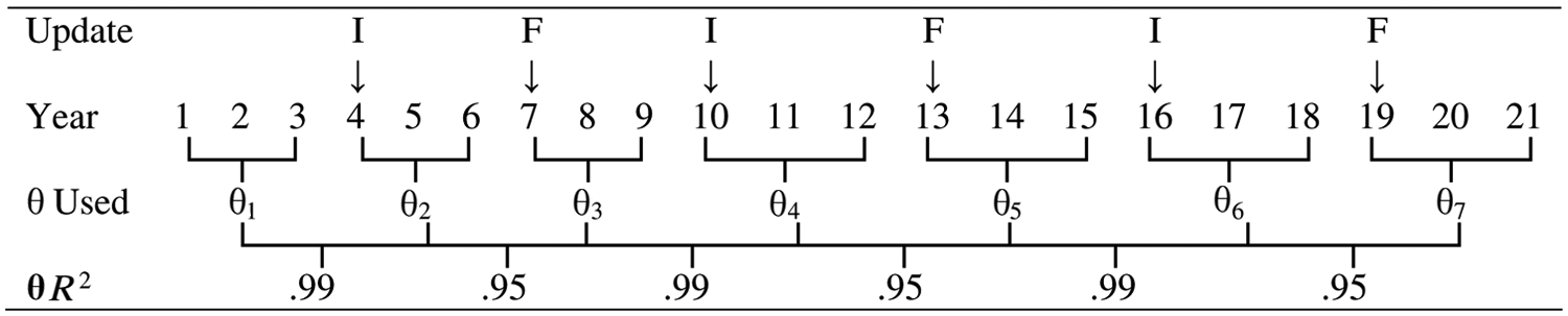
Diagram of JA updates and changes in θ by year, Δθ = 5% full JA, 1% interim JA

Analyses

Several dependent measures were used to determine how well the exam model was functioning. For the item-dependent measures, only the newly calibrated items went into the calculations. For the 1st year of the simulation, all items were involved. Only the pilot items were involved every year thereafter. Only the individuals taking the examination in a given year were involved in that year’s dependent variable calculation.

Root mean square error (RMSE) between the true and estimated item and person parameters was estimated as

RMSE ( x ) = ∑ j = 1 N ( x ^ j − x j ) 2 N ,

where N was the number of parameters, x ^ j was the estimated parameter, and x was the true value for parameter j. Bias was estimated as

Bias ( x ) = ∑ j = 1 N ( x ^ j − x j ) N .

The pass rate and the classification accuracy were also examined over years. The pass rate was simply the proportion of people whose observed θ score exceeded the predetermined cut θ. The classification accuracy was the proportion of people whose observed pass/fail decision matched their true pass/fail status as determined by their true θ values. The cut θ used to determine a pass/fail decision was 0.808. This cut θ was well below the mean of the person distribution, again because this simulation study was modeled after a particular large-scale examination program, and the program in question happened to have a relatively high pass rate. As is discussed later, the results from the pass rate and classification accuracy dependent variables can generalize to contexts with cut points that are higher than the one used in this particular study.

Person fit was also examined. It was possible that person fit would be affected as the scale drifted away from its original location. Thus, l _z person fit statistics and their means were obtained at each year. The estimation of l _z involved finding the log likelihood of a person’s response vector, subtracting the expected value of the log-likelihood function given the estimated θ, and dividing that quantity by the square root of the variance of the log-likelihood function (Karabatsos, 2003; M.-N. F. Li & Olejnik, 1997). The l _z statistic is one of the most studied IRT person fit statistics in the psychometrics literature.

Finally, correlations between estimated and true parameters were obtained at each replication. All dependent variables were first analyzed using a factorial analysis of variance to calculate η² effect sizes. After determining the factors and interactions that contributed the most, conditional means were plotted for selected conditions. The simulation and analysis of results were carried out using the base package of the statistical environment R (2.13.0; R Development Core Team, 2009).

Results

Tables 1 through 6 contain analysis of variance effect sizes for selected variables (tables of means for all dependent variables and all conditions are available online at www.arrt.org/research). Full factorial ANOVA effect sizes were calculated. The three- and four-way interactions, however, accounted for only a trivially small proportion of variance in the dependent variables. Thus, only the main effects and two-way interactions were retained in the final analysis.

OPEN IN VIEWER

Table 1.

ANOVA Effect Size Table for the Correlation Between True and Estimated θ

Factor	SS	η2
Year	14.36	0.22
PD	0.00	0.00
Δθ	36.65	0.55
DirD	0.06	0.00
Year × PD	0.00	0.00
Year ×Δθ	13.97	0.21
Year × DirD	0.01	0.00
PD ×Δθ	0.00	0.00
PD × DirD	0.03	0.00
Δθ× DirD	0.00	0.00
Residual	1.43	0.02
Total	66.52

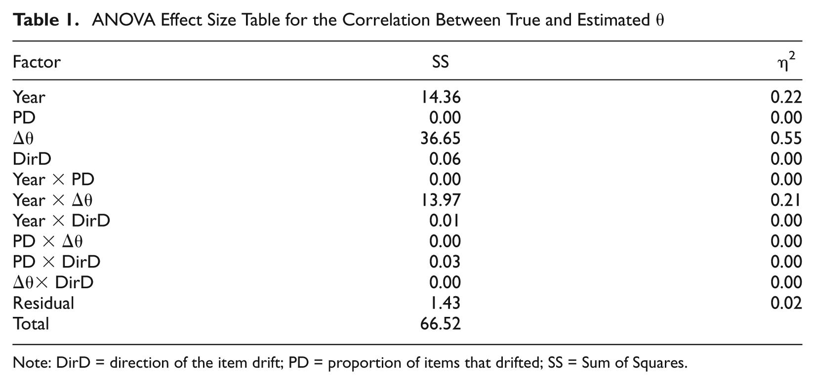
Note: DirD = direction of the item drift; PD = proportion of items that drifted; SS = Sum of Squares.

Table 1 contains the ANOVA table for θ correlation. The main effects of year and Δθ and the interaction of year and Δθ together accounted for about 98% of the variance in the θ correlation. Figure 2 contains a plot of the mean θ correlations conditional on year and Δθ. There are two interesting features of the data highlighted by this graph. First, practice analyses involving only a 1% change in the latent trait did not have a large effect on the θ correlation, but practice analyses involving 10% change did have a substantial impact on the recovery of θ. Second, the recovery of θ showed an interesting pattern of rising and falling. Recovery immediately declined after a practice analysis but climbed in subsequent years. The improvement in θ recovery in the later 2 years of a practice analysis was due to the recently calibrated pilot items being available for use on the exams. These items more accurately estimated θ than items calibrated many years earlier.

OPEN IN VIEWER

Figure 2.

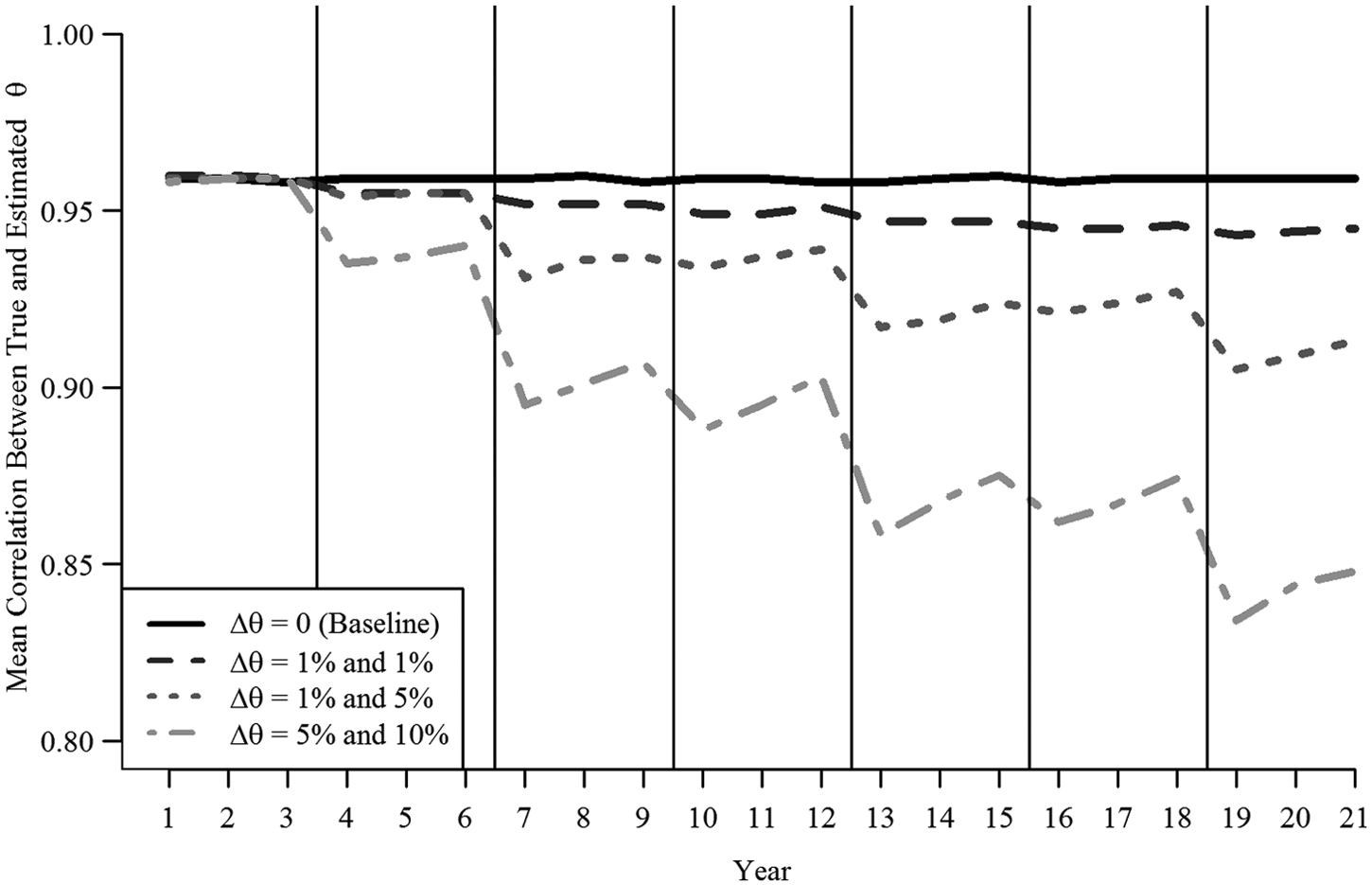
Plot of the mean correlations between true and estimated θ conditional on Δθ and year, PD = 0

Table 2 contains the effect sizes for θ RMSE. The main effects of year and Δθ and the interaction of year and Δθ together accounted for about 69% of the variance in the θ RMSE. The main effect of PD accounted for about 10% of the variance, indicating that as PD increased, RMSE also increased. Figure 3 contains a plot of the mean θ RMSEs conditional on Δθ and year. The pattern of results was virtually the same as the results in Figure 2, with large JA changes causing worse θ recovery but improving recovery in the later 2 years of a JA cycle.

OPEN IN VIEWER

Table 2.

ANOVA Effect Size Table for θ RMSE

Factor	SS	η2
Year	94.91	0.30
PD	32.47	0.10
Δθ	94.13	0.30
DirD	19.36	0.06
Year × PD	8.97	0.03
Year ×Δθ	29.55	0.09
Year × DirD	5.60	0.02
PD ×Δθ	0.59	0.00
PD × DirD	16.95	0.05
Δθ× DirD	0.42	0.00
Residual	13.22	0.04
Total	316.17

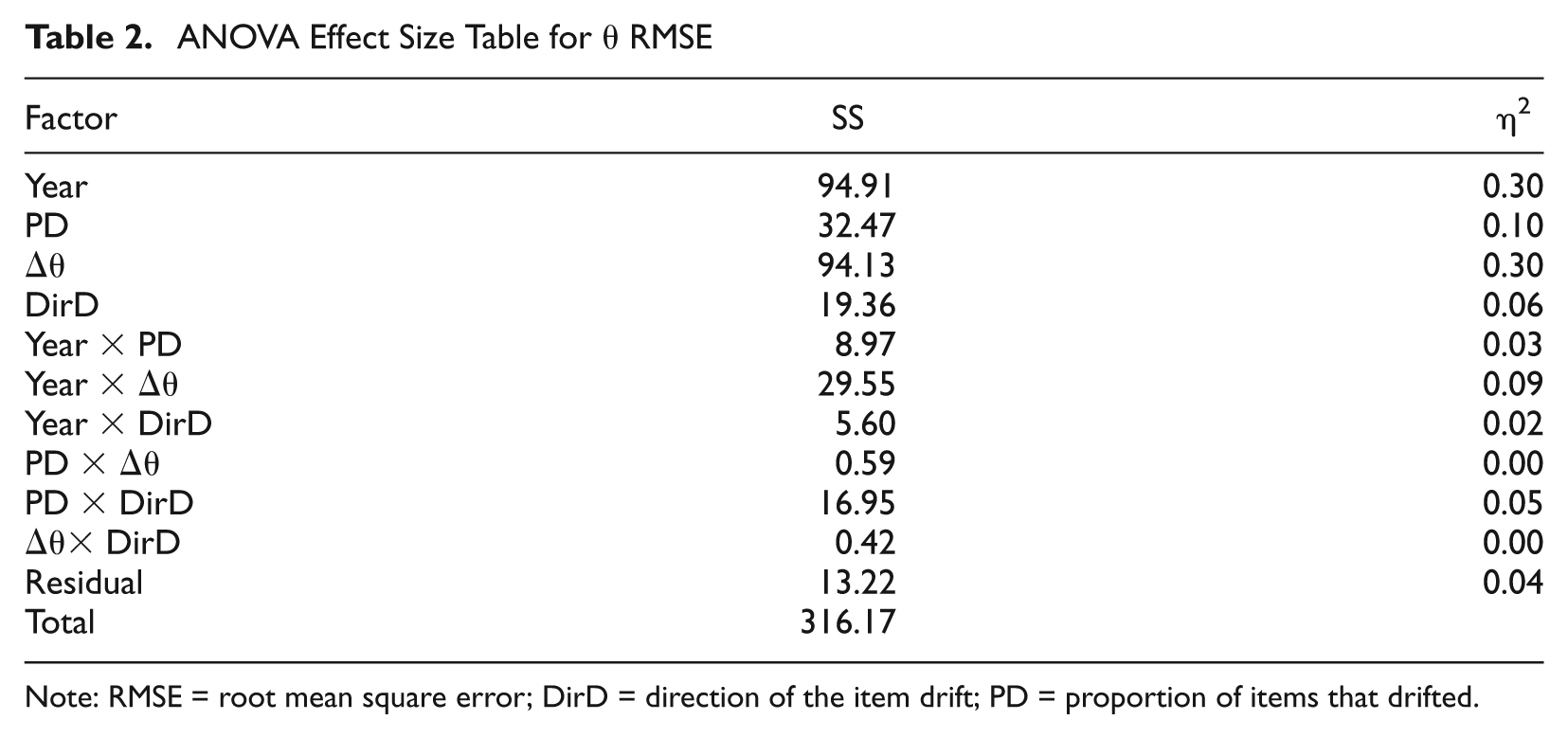
Note: RMSE = root mean square error; DirD = direction of the item drift; PD = proportion of items that drifted.

OPEN IN VIEWER

Figure 3.

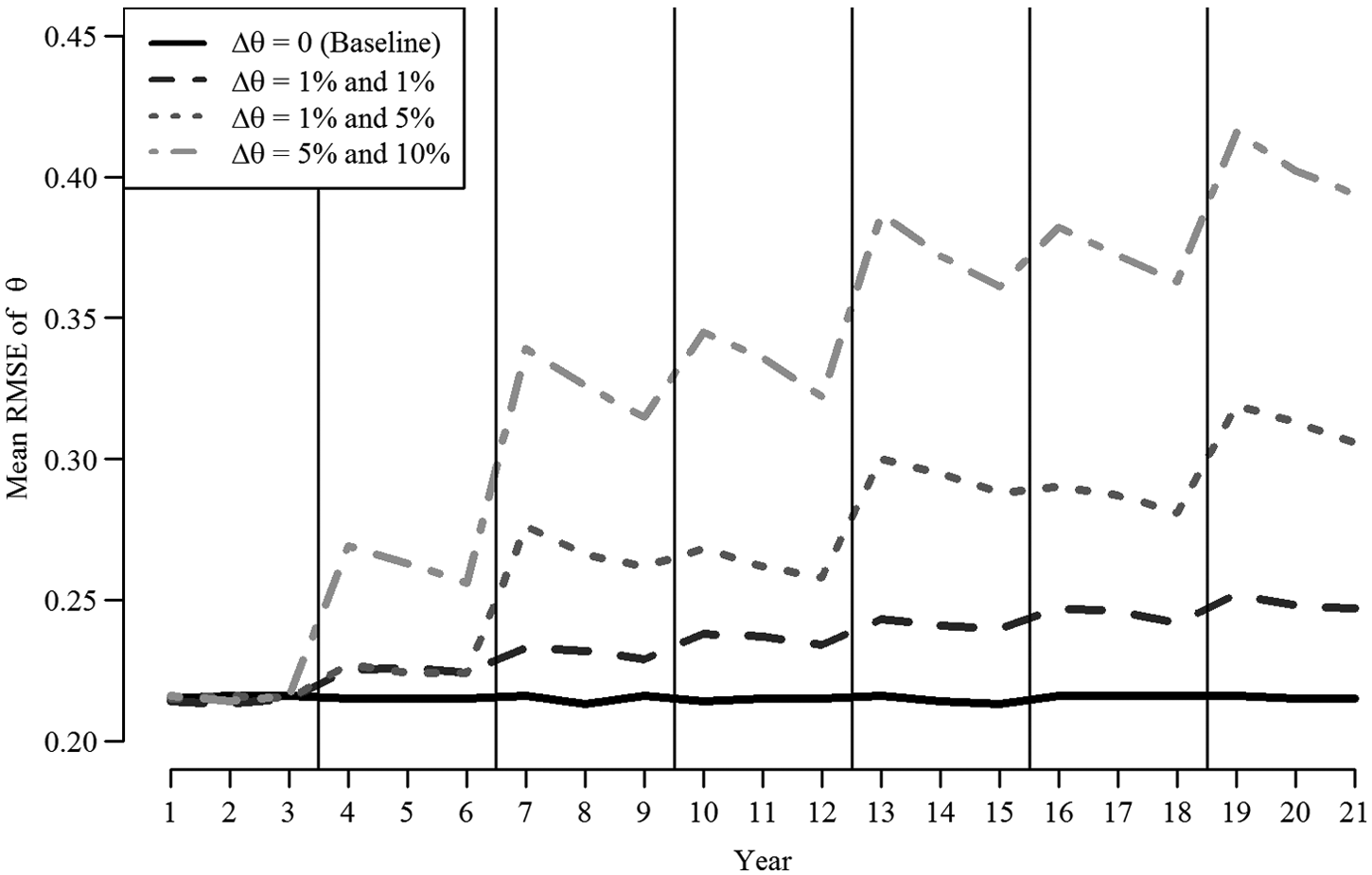
Plot of the mean θ RMSEs conditional on Δθ and year, PD = 0

Table 3 contains the effect sizes for θ bias. The main effect of DirD and the interactions between DirD and PD along with DirD and year account for about 91% of the variance in bias. Figure 4 contains a plot of the mean θ bias conditional on DirD, PD, and year. The bias results show a fanlike pattern instead of the rising and falling pattern seen in the correlation and RMSE dependent variables. There are two notable features about this figure. First, item drift did not have much of an adverse effect on θ recovery if some of the items drifted up and some drifted down. The lines for the “DirD = Both” conditions were quite close to the baseline condition throughout across years. Second, drifting the items up (more difficult) had more of a biasing effect than drifting items down. Because the pool of items was already relatively easy, item drift in the easier direction did not affect scores as much as drift in the difficult direction, although easy and difficult drift had a substantial effect on the estimation of θ.

OPEN IN VIEWER

Table 3.

ANOVA Effect Size Table for Bias in θ

Factor	SS	η2
Year	5.78	0.01
PD	9.45	0.01
Δθ	0.13	0.00
DirD	552.68	0.55
Year × PD	2.05	0.00
Year ×Δθ	0.08	0.00
Year × DirD	95.66	0.09
PD ×Δθ	0.04	0.00
PD × DirD	273.92	0.27
Δθ× DirD	0.00	0.00
Residual	71.21	0.07
Total	1,011.00

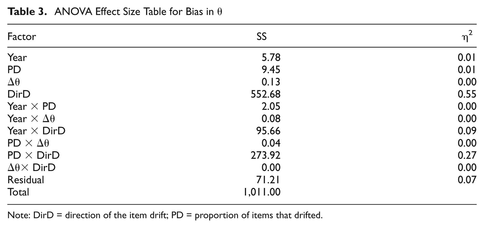
Note: DirD = direction of the item drift; PD = proportion of items that drifted.

OPEN IN VIEWER

Figure 4.

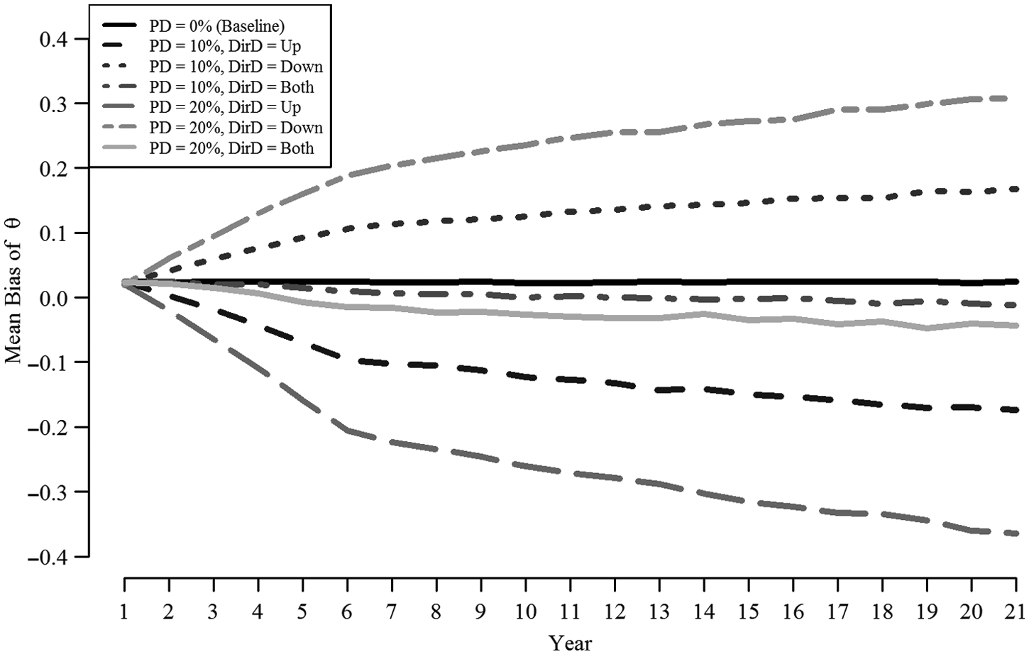
Plot of the mean θ bias conditional on DirD, PD, and year, Δθ = 0

The results for pass rate were quite similar to the results for θ bias, with drift in both directions having very little effect but drift in one direction having a substantial effect. The conditions causing positive θ bias also caused pass rates to increase, whereas conditions causing negative θ bias caused pass rates to decrease.

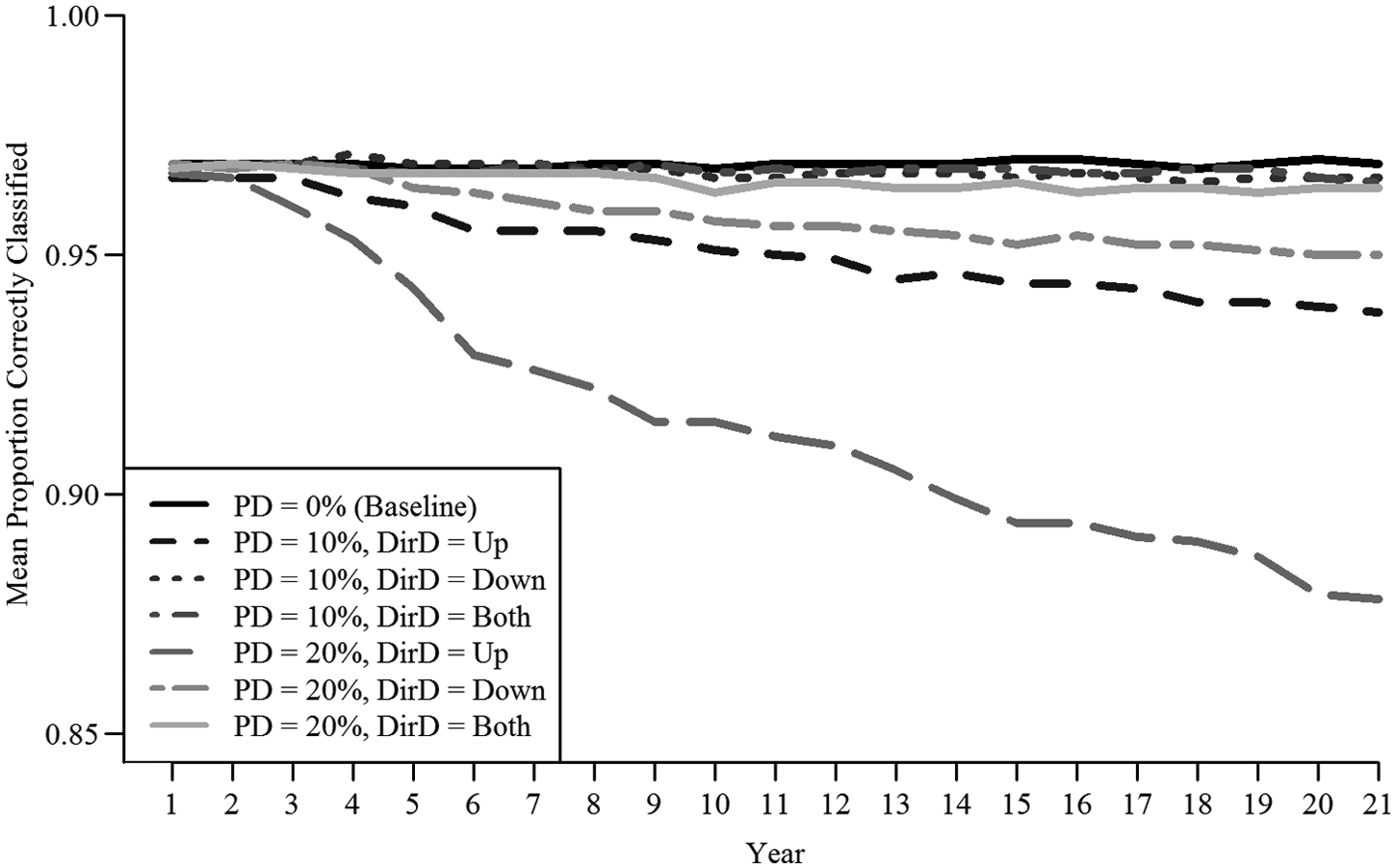
Table 4 contains the effect sizes for classification accuracy. The four main effects together explained about 61% of the variance, with the interaction between PD and DirD accounting for an additional 13% of the variance in classification accuracy. Figure 5 contains a plot of the mean θ bias conditional on DirD, PD, and year. In the conditions where some items drifted in the difficult and some in the easy direction, virtually no difference in classification accuracy is evident, compared with the baseline. In the conditions where items drifted in the negative (easier) direction, the impact was much less dramatic. This was a result of the location of the cut point. Because the cut point was low relative to the distribution of θ, the overall true pass rate was high. Thus, the decision to classify a person as failing was much “riskier” than classifying a person as passing. When items drifted easier, there were fewer “risky” failing decisions being made. Examinees were more often classified as failing when items drifted in the difficult direction. If the cut point were high (i.e., lower overall pass rate), the opposite trend would have been noted. Cut points that lead to pass rates near 50% would be equally affected by positive and negative item drift. The plot of classification accuracy conditional on Δθ and year (not included) followed the same pattern as the θ correlation plot.

OPEN IN VIEWER

Table 4.

ANOVA Effect Size Table for Classification Accuracy

Factor	SS	η2
Year	5.25	0.20
PD	2.82	0.11
Δθ	3.41	0.13
DirD	4.59	0.17
Year × PD	0.78	0.03
Year ×Δθ	1.04	0.04
Year × DirD	1.14	0.04
PD ×Δθ	0.08	0.00
PD × DirD	3.36	0.13
Δθ× DirD	0.05	0.00
Residual	4.19	0.16
Total	26.70

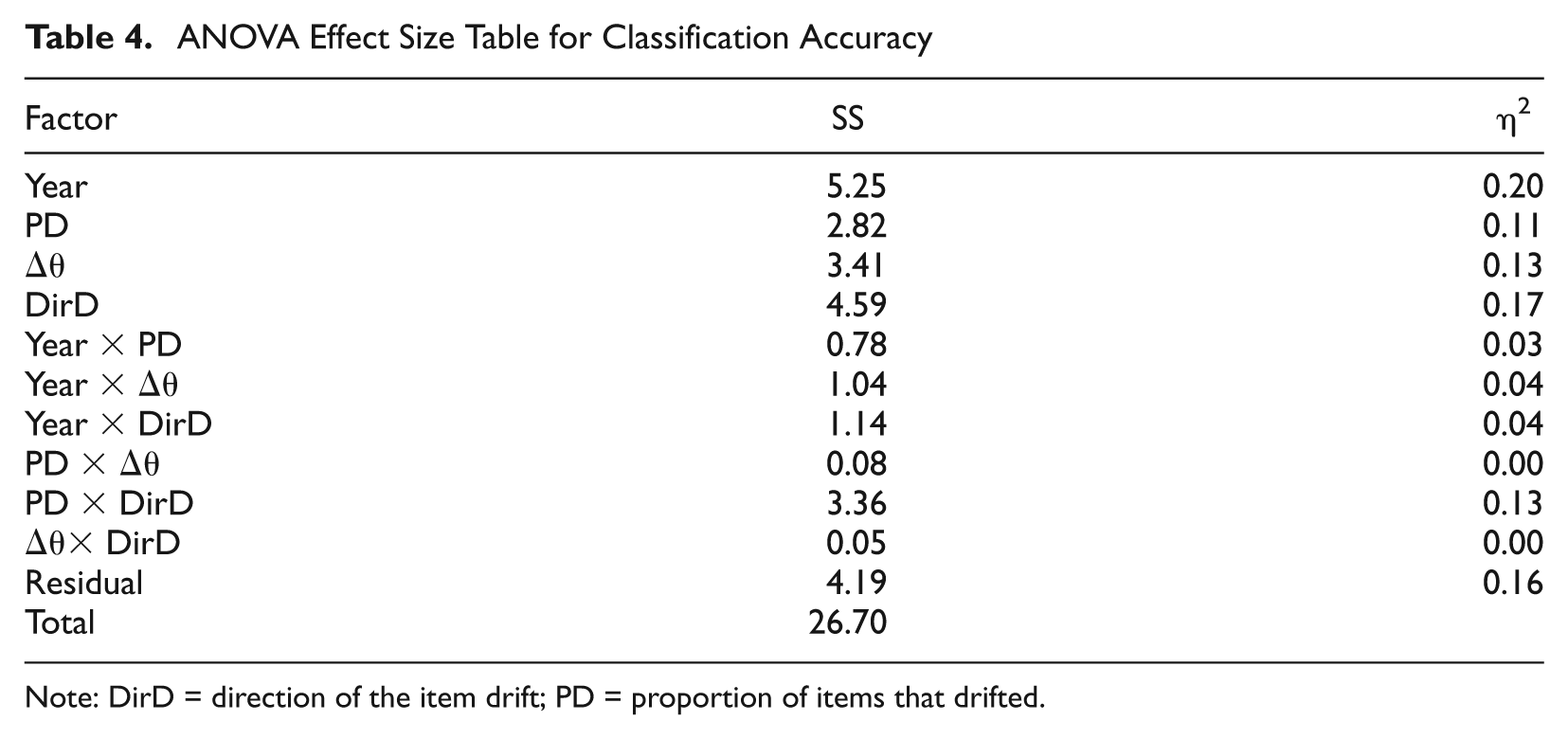
Note: DirD = direction of the item drift; PD = proportion of items that drifted.

OPEN IN VIEWER

Figure 5.

Plot of the classification accuracy conditional on DirD, PD, and year, Δθ = 0

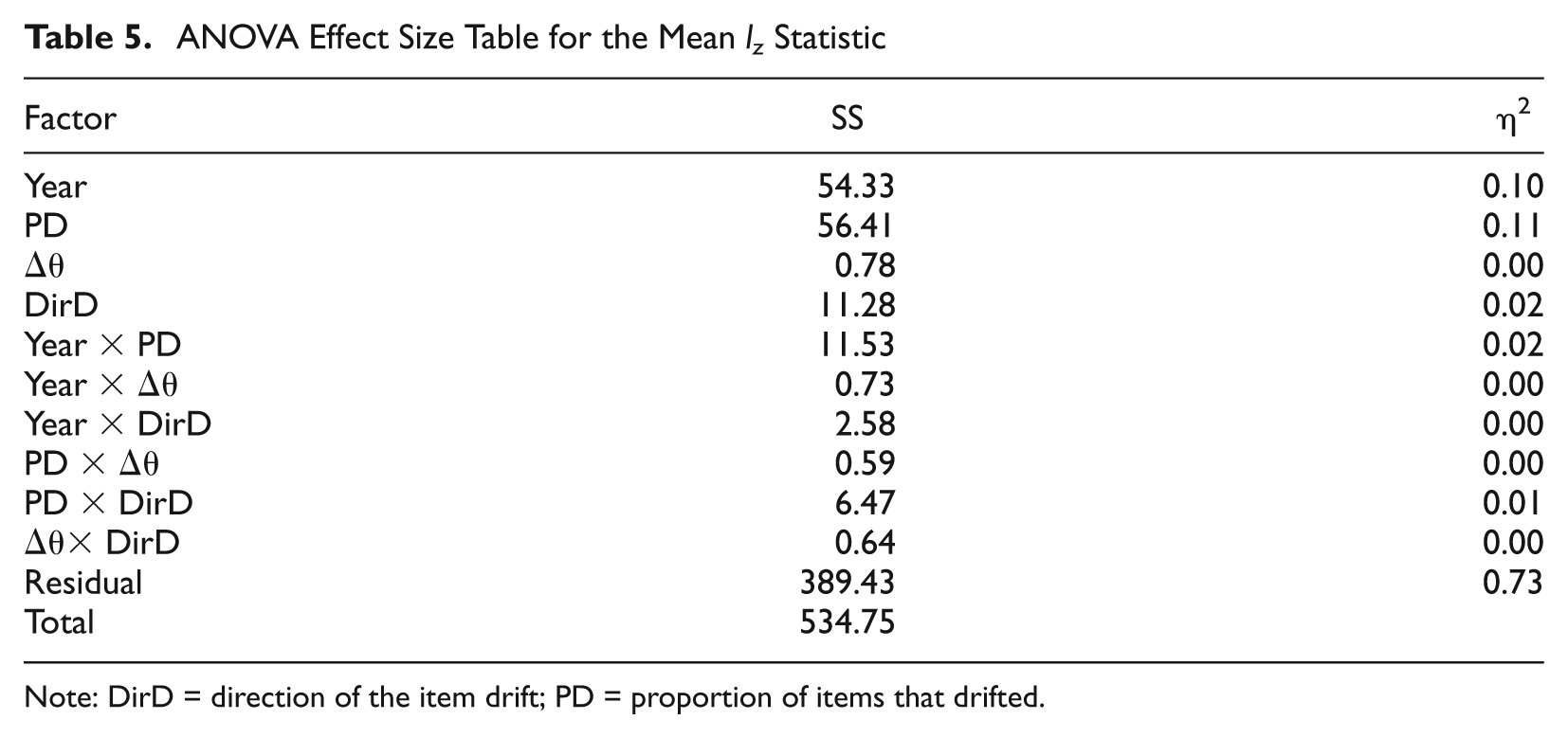
Table 5 contains the effect sizes for the mean l _z statistic. The main effects of year and PD only accounted for about 21% of the variance. The residual variance dwarfed the variance explainable by all the factors and interactions combined. As the number of years and the drift proportion increased, there was a very slight decrease in the person-fit statistic. The decrease trend was quite small, however, compared with the random year-to-year increases and decreases in the fit statistic. It appears that the mean l _z statistic was not very sensitive to overall shifts in the measurement scale.

OPEN IN VIEWER

Table 5.

ANOVA Effect Size Table for the Mean l _z Statistic

Factor	SS	η2
Year	54.33	0.10
PD	56.41	0.11
Δθ	0.78	0.00
DirD	11.28	0.02
Year × PD	11.53	0.02
Year ×Δθ	0.73	0.00
Year × DirD	2.58	0.00
PD ×Δθ	0.59	0.00
PD × DirD	6.47	0.01
Δθ× DirD	0.64	0.00
Residual	389.43	0.73
Total	534.75

Note: DirD = direction of the item drift; PD = proportion of items that drifted.

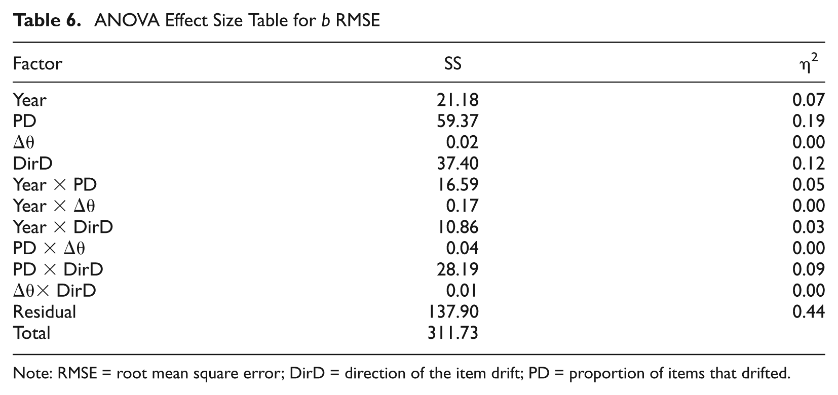
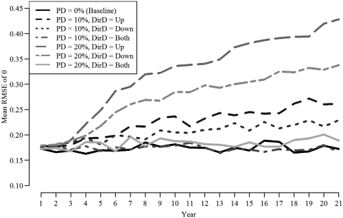
Dependent variables for the item parameters were also recorded; however, these results were not as informative as the person parameter results. No factor accounted for more than 2% of the variance in the correlation between true and estimated b. The results for bias in b were virtually identical to the results for θ bias. The main effects of PD, DirD, and the interaction between the two accounted for about 40% of the variance as seen in Table 6. The pattern for b RMSE means shown in Figure 6 reinforces the conclusion that, for a testing program where items are relatively easy, drift in the difficult direction has a more detrimental effect than drift in the easy direction.

OPEN IN VIEWER

Table 6.

ANOVA Effect Size Table for b RMSE

Factor	SS	η2
Year	21.18	0.07
PD	59.37	0.19
Δθ	0.02	0.00
DirD	37.40	0.12
Year × PD	16.59	0.05
Year ×Δθ	0.17	0.00
Year × DirD	10.86	0.03
PD ×Δθ	0.04	0.00
PD × DirD	28.19	0.09
Δθ× DirD	0.01	0.00
Residual	137.90	0.44
Total	311.73

Note: RMSE = root mean square error; DirD = direction of the item drift; PD = proportion of items that drifted.

OPEN IN VIEWER

Figure 6.

Plot of the b RMSE conditional on DirD, PD, and year, Δθ = 0

Discussion

This research simulated a testing situation where the item difficulties and latent trait drifted over time. The results showed that a Rasch IRT scale can maintain near baseline recovery properties if the changes in the latent trait over time are small. The Rasch scale also maintained good recovery of item and person parameters if there was equal item drift in both directions. However, an IRT Rasch scale cannot be carried forward indefinitely without major consequences to person and item parameter estimation. With about 10% of items drifting, classification accuracy stayed consistently below 95% after the 15-year mark (see Figure 5). In terms of changes in test content specifications or the material being tested over time, drift in the latent trait of 1% and 5% seemed to become problematic after Year 18, when the correlation between true and estimated theta had decreased by about .05 (see Figure 2). Thus, under conditions of relatively little item drift and small to moderate periodic changes in the latent trait, a Rasch scale may remain stable for 15 years, ±3.

Recovery of θ generally degraded the 1st year following a shift in the latent trait. Recovery then rebounded in the following 2 years. This rebound can be attributed to the availability of newly piloted items, which reflected the most recent changes in the latent trait. These newer items more accurately estimated the latest θ than did items that had been piloted in previous JA cycles. This finding suggests that when constructing new test forms, estimation of θ may be improved through the use of as many newly piloted items as possible.

Whereas limited IPD and trait drift increased the longevity of the scale, substantial item drift or large changes in the latent trait dramatically reduced the longevity of the scale (see Figures 1-6). However, regular maintenance of a measurement scale in practice using drift detection methods will likely improve scale longevity. Thus, scales covering content that is frequently revised and affected by changes in technology, for example, may still remain stable if drifting items are detected and revised or removed. This study was concerned primarily with scale stability in the absence of maintenance. It provides a worst-case scenario or baseline indication of how shifts in item difficulty and latent trait can affect parameter recovery. Future research should examine scale stability in conjunction with the use of IPD detection techniques, including, for example, time-dependent IRT models such as those demonstrated by Bock et al. (1988).

Practitioners may wonder how to determine the status of their own testing program in terms of the variables manipulated in this study. There are numerous methods for doing this, but only a few are discussed here. To determine the amount and direction of item drift, psychometricians could look at item proportions correct over time. If there are substantial changes over time to an item, then the item is drifting. A psychometrician using fixed item anchor calibration could also use the item displacement index calculated by WINSTEPS (Linacre, 2009). One could also use any number of other DIF detection methods (Holland & Wainer, 1993). One could also use test characteristic curve methods to anchor the scale over time, which gives the user the ability to find outlying items in the scale-linking process. This index is a measure of how much the item b value would change if the item were estimated instead of fixed. Determining the level of changes from a JA is a much more difficult topic. Future research should consider how best to quantify this type of change, using test data and ratings from subject matter experts.

In the present study, the Rasch model was examined under specific test design conditions using simulated data. As a result, the generalizability of results centers mainly on job-related testing programs using the Rasch model. Future research on IRT scale stability should also consider other IRT models. More complex models, such as the 2PL or 3PL, polytomous, or multidimensional IRT models, would result in differing measurement scales, and IPD and latent trait drift may affect these scales in different ways, particularly if parameters other than the b parameter are drifting. Future research should also consider related contexts, such as educational testing programs, where latent trait changes may be due to factors such as updates to the curriculum or instructional approach and advancements in learning technology. Such educational shifts may also be a concern to certification testing, as many certifications have educational requirements that candidates must fulfill to sit for the exam. Although results from the present study can inform the discussion of scale stability in educational measurement, the regularity of the JA cycle, and the corresponding latent trait change, is unique to certification/licensure/job-related testing.

In conclusion, although there is no rule for when to reset an IRT scale, this study offers practical guidance in determining the number of years before a variety of dependent variables cross thresholds of unacceptability. The generalizability of these results depends on the similarity between the conditions studied here and those found in a testing program. For a particular program, the decision of when to reset the scale should be based on the amount of acceptable loss in the accuracy of estimating θ, and the psychometric conditions under which the loss occurs. In examining scale stability, practitioners must consider the amount and direction of item drift, and the amount of change in the latent trait that is occurring. Although programs may maintain an IRT scale over many years for the sake of comparability and consistency in decision making and score reporting, this study shows that functionality and stability eventually require recalibration.