A Note on the Item Information Function of the Four-Parameter Logistic Model

Abstract

This article focuses on four-parameter logistic (4PL) model as an extension of the usual three-parameter logistic (3PL) model with an upper asymptote possibly different from 1. For a given item with fixed item parameters, Lord derived the value of the latent ability level that maximizes the item information function under the 3PL model. The purpose of this article is to extend this result to the 4PL model. A generic and algebraic method is developed for that purpose. The result is practically illustrated by an example and several potential applications of this result are outlined.

Keywords

item response theory four-parameter logistic model item information function maximization

In the field of dichotomous item response theory (IRT) models, the three-parameter logistic (3PL) model (Birnbaum, 1968) and the simpler one- and two-parameter logistic (1PL and 2PL) models have received most attention in the past decades. However, an extended version of the 3PL model was also suggested, by allowing an upper asymptote possibly smaller than 1. This four-parameter logistic (4PL) model, early proposed by Barton and Lord (1981) and barely mentioned by Hambleton and Swaminathan (1985), did not receive a lot of attention until recently. As Loken and Rulison (2010) pointed out, the strong dominancy of the 3PL model in the literature, the lack of consensus on its usefulness, and the technical difficulty in estimating the upper asymptote accurately, are strong arguments against the use of the 4PL model.

Despite these conceptual drawbacks, the 4PL model was reconsidered recently in the literature. One reason is the recent improvement in computational power and resources, together with the development of accurate statistical modeling software. Some early arguments toward accurate estimation of the upper asymptote can be found in Linacre (2004) and Rupp (2003). Very recently, Loken and Rulison (2010) developed a Bayesian framework to calibrate the items under a 4PL model, by using a Markov chain Monte Carlo (MCMC) approach and the WinBUGS software (Lunn, Thomas, Best, & Spiegelhalter, 2000). This software was obviously not available when the 4PL model was suggested first, and it constitutes a major breakthrough toward a broader consideration of that model for practical purposes.

Moreover, the main asset of the 4PL model is that it allows a nonzero probability of answering the item incorrectly for highly able respondents. This asset was exploited by Rulison and Loken (2009) in the computerized adaptive testing (CAT) environment. More precisely, they showed that the impact of early mistakes made by highly able respondents (due to stress for instance) can be strongly reduced with the 4PL model, and that fewer items need to be administered to cancel the related ability estimation bias (with respect to the 3PL model). Subsequent studies of the usefulness of the 4PL model in the CAT framework were performed by Green (2011); Liao, Ho, Yen, and Cheng (2012); and Yen, Ho, Liao, Chen, and Kuo (2012). Moreover, the 4PL model was recently introduced as the baseline IRT model for CAT generation in the R package catR (Magis & Raîche, 2012). It is also worth mentioning that the 4PL model will probably become a potentially useful model to detect person fit, and especially careless or inattention patterns (Tendeiro & Meijer, 2012).

The asset of this “upper asymptote” characteristic was also illustrated in several applied research fields. One example comes from the criminology context. Osgood, McMorris, and Potenza (2002) made use of a 2PL model to analyze a self-report delinquency scale and noticed that the use of a 4PL model (or any other model with an upper asymptote parameter), might permit to catch the propensity of most delinquent youth not to report some delinquent acts (see also Loken & Rulison, 2010). In the field of psychopathology research, Reise and Waller (2003; see also Waller & Reise, 2009) advocated for the need for nonstandard IRT models to analyze clinical and personality instruments. The genetics research field was also considered for applications of IRT models, and especially the 4PL model. Tavares, de Andrade, and Pereira (2004) proposed a 4PL model to allow low-disposition individuals to have the gene activated (which requires a lower asymptote parameter) as well as high-disposition individuals not to have the gene activated (by including an upper asymptote parameter).

As the 4PL model did not receive much attention yet, these practical examples are not numerous. However, they clearly highlight the potential and usefulness of this model, both from a methodological point of view and for practical purposes. It can therefore be expected that future research will focus on the 4PL model and promote it as a competing model in some particular situations.

The aim of this note is to focus on one specific but important aspect of the 4PL model that was not investigated yet: the characterization of its item information function. More precisely, deriving its maximum value, and the corresponding optimal latent ability yielding this maximum, might be of interest to the understanding of the model and also for practical applications. Among them, CAT (Chang & Yin, 2008; Rulison & Loken, 2009) and robust estimation of ability (Magis, 2012; Mislevy & Bock, 1982; Schuster & Yuan, 2011) are two promising fields of applications for the present developments. They are discussed in detail at the end of this note.

Deriving the optimal ability level that maximizes the information function is straightforward under the 1PL and 2PL models. With the 3PL model, the solution was provided by Birnbaum (1968; see also Lord, 1980). This article extends this solution to the 4PL model and draws parallelisms between the 4PL and simpler IRT models.

The Model and Its Information Function

Let us focus on any particular item j from a set of J items. The general form of the 4PL model is the following:

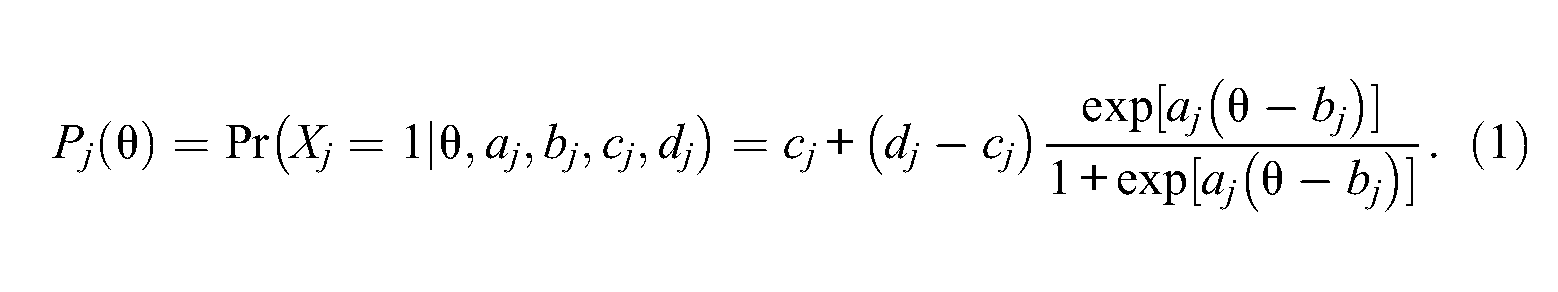
P_{j} (θ) = \Pr (X_{j} = 1 | θ, a_{j}, b_{j}, c_{j}, d_{j}) = c_{j} + (d_{j} - c_{j}) \frac{exp [a_{j} (θ - b_{j})]}{1 + exp [a_{j} (θ - b_{j})]} .

In this model, X_j is the binary response of the respondent with latent ability level θ to item j, coded as 1 for a correct response and 0 for an incorrect one. Moreover, $(a_{j}, b_{j}, c_{j}, d_{j})$ is the vector of item parameters, that is, the discrimination level, the difficulty level, the lower asymptote (pseudoguessing level), and the upper asymptote (inattention level), respectively. In addition to the three usual item parameters, the upper asymptote allows that highly able respondents may nevertheless answer the item incorrectly (because of stress, tiredness, or inattention, for instance). In its general form, the 4PL model allows a different upper asymptote per item, while originally Barton and Lord (1981) suggested a common upper asymptote for all items; that is, $d_{j} = d$ for all j.

In this article, it is assumed that all four item parameters are fixed at known values. As a good practice, one may think about item parameter values as having arisen from previous model fit or by precalibration of the model to the data under study. This could be achieved, for instance, by using the Bayesian estimation approach recently proposed by Loken and Rulison (2010). Thus, only the latent ability level remains unknown and will constitute our variable of interest in the following discussion. Moreover, it is assumed that $c_{j} \in (0; 0.5)$ and $d_{j} \in (0.5; 1)$ . This ensures that the response probability $P_{j} (θ)$ is strictly increasing with θ as the difference $d_{j} - c_{j}$ is strictly positive.

One important feature of IRT models is the item information function. It is a mathematical function of the ability level θ and the item parameters that describes how informative the item is at any given θ level. Very easy items are usually more informative at low ability levels whereas highly difficult and discriminating items are more informative for larger ability levels. The general form of the item information function, given any dichotomous IRT model described by a response probability $P_{j} (θ)$ , is given by (Lord, 1980, p. 72):

I_{j} (θ) = \frac{P_{j}^{'} {(θ)}^{2}}{P_{j} (θ) Q_{j} (θ)},

where $Q_{j} (θ) = 1 - P_{j} (θ)$ and $P_{j}^{'} (θ)$ is the first derivative of $P_{j} (θ)$ with respect to θ. In order to simplify the notations, and because the aim of this article is to focus on a single item information function at the time, the item subscript j is removed from the rest of the article.

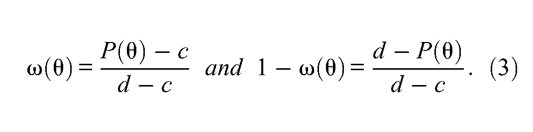
Before focusing on the item information function more in detail, let us rewrite it in a simpler way that does not involve the first derivative $P_{j}^{'} (θ)$ . Set $ω (θ) = \exp [a (θ - b)] / {1 + \exp [a (θ - b)]}$ , so that $P (θ) = c + (d - c) ω (θ)$ or

ω (θ) = \frac{P (θ) - c}{d - c} and 1 - ω (θ) = \frac{d - P (θ)}{d - c} .

The first derivative of $ω (θ)$ with respect to θ is

ω^{'} (θ) = \frac{a \exp [a (θ - b)]}{{1 + \exp [a (θ - b)]}^{2}} = a ω (θ) [1 - ω (θ)],

by definition of $ω (θ)$ , so that

P^{'} (θ) = (d - c) ω^{'} (θ) = \frac{a}{d - c} [P (θ) - c] [d - P (θ)],

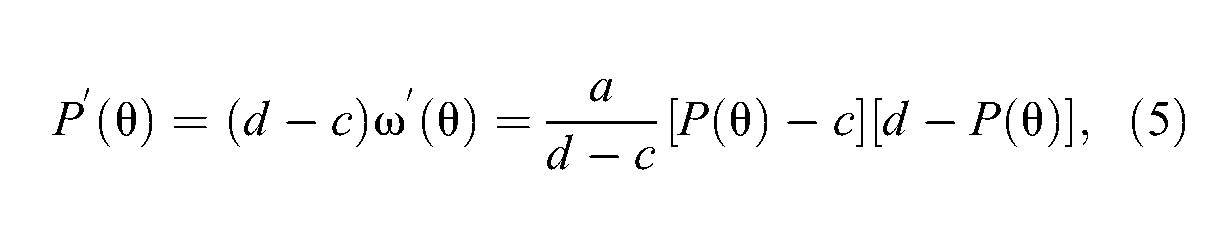
by using Equation 3. In sum, the item information function in Equation 2 can be directly related to the response probability of Equation 1 as follows:

I (θ) = \frac{a^{2} {[P (θ) - c]}^{2} {[d - P (θ)]}^{2}}{{(d - c)}^{2} P (θ) [1 - P (θ)]} .

The central result of this article is that the item information function has a single maximum value, corresponding to a specific $θ^{*}$ ability level, and the objective is to determine $θ^{*}$ algebraically. To this end, the form of the information function given by Equation 6 will be most useful. The mathematical derivations are detailed in the next section.

Maximizing the Information

First of all, rather than maximizing the information function with respect to θ directly, one will maximize it with respect to P(θ). This will greatly simplify the mathematical derivations, and because P(θ) is a strictly increasing function of θ, it will be straightforward to obtain the value of $θ^{*}$ , as will be shown later on. Set x = P(θ) and

I (x) = \frac{a^{2} {(x - c)}^{2} {(d - x)}^{2}}{{(d - c)}^{2} x (1 - x)},

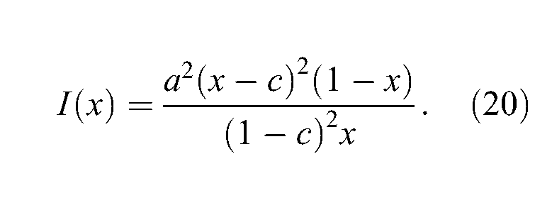
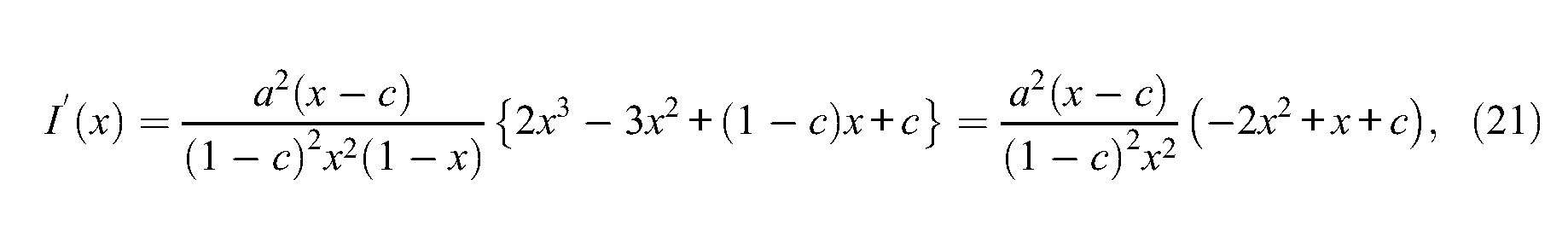
as the function to be maximized for $x \in (c; d)$ , according to Equation 6 and the definition of x.

A long but straightforward calculation leads to the first derivative of I(x) with respect to x:

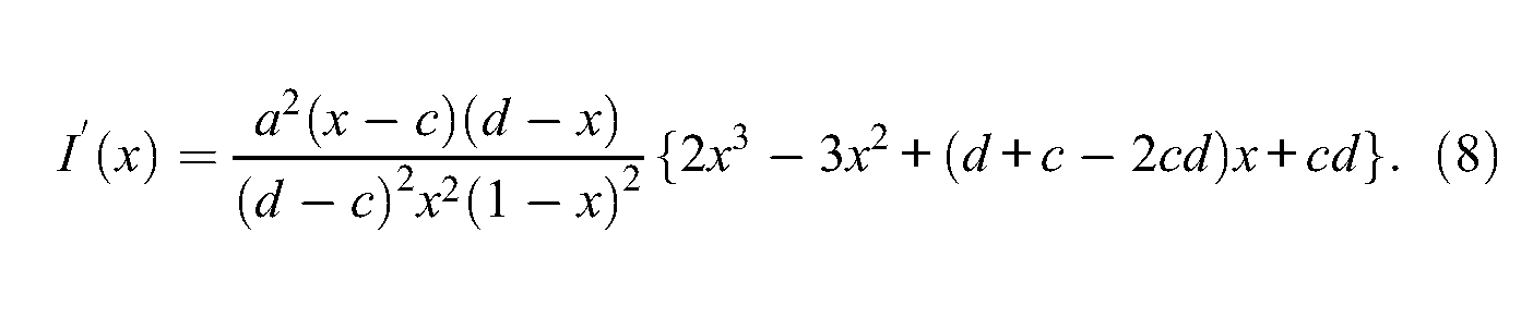
I^{'} (x) = \frac{a^{2} (x - c) (d - x)}{{(d - c)}^{2} x^{2} {(1 - x)}^{2}} {2 x^{3} - 3 x^{2} + (d + c - 2 cd) x + cd} .

As x takes values in (c; d), the sign of this derivative is therefore determined by the sign of the polynomial

p (x) = 2 x^{3} - 3 x^{2} + (d + c - 2 cd) x + cd,

which may have at most three real roots, that is, the number of times the polynomial function crosses the horizontal axis set by p(x) = 0.

To further characterize p(x), and hence to extract useful information about the information function, for the moment let us consider x as a real value on the whole real axis. The first derivative of p(x) with respect to x is equal to $p^{'} (x) = 6 x^{2} - 6 x + (d + c - 2 cd)$ and has two real roots given by

y_{1} = \frac{1}{2} - \frac{\sqrt{36 - 24 (c + d - 2 cd)}}{12} and y_{2} = \frac{1}{2} + \frac{\sqrt{36 - 24 (c + d - 2 cd)}}{12} .

Note that $c + d - 2 cd = c (1 - d) + d (1 - c)$ and is thus smaller than 1 as all terms are smaller than 1, so the roots y₁ and y₂ are well defined. The general shape of p(x) is therefore the following: It increases first for increasing x up to y₁, then it decreases between y₁ and y₂, and reincreases then for increasing values of x larger than y₂. Moreover, as

lim_{x \to \pm \infty} p (x) = \pm \infty, p (c) = 2 c (1 - c) (d - c) > 0 and p (d) = 2 d (1 - d) (c - d) < 0,

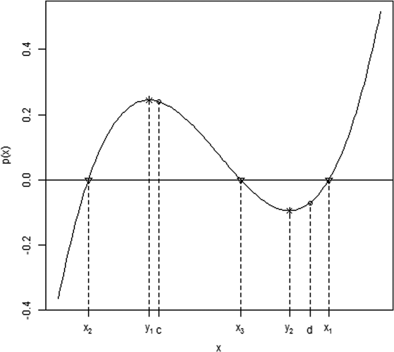
and because the function p(x) is continuous on the whole real scale, one may conclude from the intermediate value theorem that p(x) has actually three real roots, belonging respectively to the intervals $(- \infty; c)$ , $(c; d)$ , and $(d; + \infty)$ . Back to the 4PL model framework, this means that a single root belongs to the allowed interval (c; d), which implies that the information function has a single maximum value. Figure 1 provides an illustration of the shape of p(x) with c = 0.2 and d = 0.95. The roots y₁ and y₂ are displayed with star symbols, together with c and d parameters and the three roots of p(x) denoted by x₁, x₂, and x₃ (see the following sections).

Figure 1.

Graphical illustration of the polynomial p(x) with c = 0.2 and d = 0.95.

Now, to determine the roots of the polynomial p(x), one makes use of the so-called Cardano’s method to derive the roots of any third-order polynomial. The main steps of the method are described hereafter without proof; further details can be found in Jacobson (1985). Set first α, β, γ, and δ as the numeric coefficients of the polynomial p(x); that is,

α = 2, β = - 3, γ = c + d - 2 cd, δ = cd,

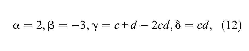
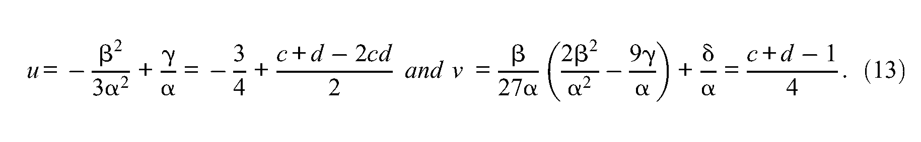
according to Equation 9. Set moreover $z = x + β / (3 α) = x - 0.5$ , so that the polynomial p(x) can be rewritten as $p (z) = z^{3} + uz + v$ with

u = - \frac{β^{2}}{3 α^{2}} + \frac{γ}{α} = - \frac{3}{4} + \frac{c + d - 2 cd}{2} and v = \frac{β}{27 α} (\frac{2 β^{2}}{α^{2}} - \frac{9 γ}{α}) + \frac{δ}{α} = \frac{c + d - 1}{4} .

The sign of the discriminant $δ = v^{2} + 4 u^{3} / 27$ of polynomial p(z) determines the number of real roots. As p(z) has three real roots (see earlier discussion), this means that $Δ < 0$ and the roots of p(z) are given by

z_{k} = 2 \sqrt{\frac{- u}{3}} \cos {\frac{1}{3} acos (- \frac{v}{2} \sqrt{\frac{27}{- u^{3}}}) + \frac{2 (k - 1) π}{3}}, k = 0, 1, 2 .

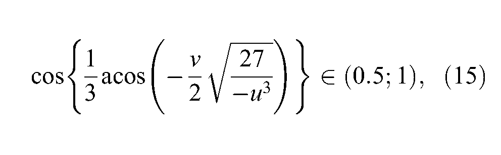
Eventually, the three real roots of polynomial p(x) are given by $x_{k} = z_{k} + 0.5$ (k = 0, 1, 2) by definition of z.

Thus, the root of polynomial p(x) that belongs to (c; d) is one of the three roots $x_{k}$ described above. To determine it, notice first that acos(t) belongs to (0; π) for any $t \in (- 1; 1)$ . It is then straightforward to notice that

\cos {\frac{1}{3} acos (- \frac{v}{2} \sqrt{\frac{27}{- u^{3}}})} \in (0.5; 1),

\cos {\frac{1}{3} acos (- \frac{v}{2} \sqrt{\frac{27}{- u^{3}}}) + \frac{2 π}{3}} \in (- 1; - 0.5),

and

\cos {\frac{1}{3} acos (- \frac{v}{2} \sqrt{\frac{27}{- u^{3}}}) + \frac{4 π}{3}} \in (- 0.5; 0.5) .

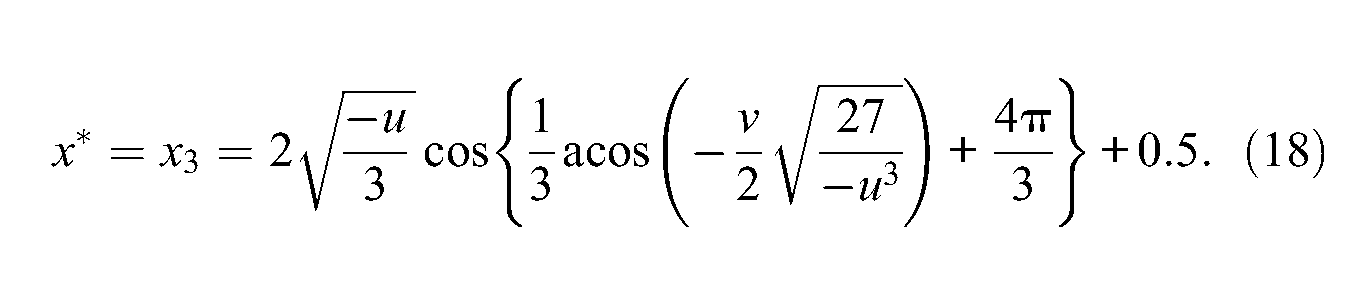
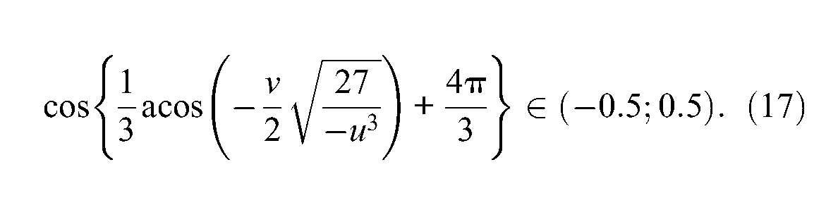
This implies finally that $z_{2} < z_{3} < z_{1}$ and $x_{2} < x_{3} < x_{1}$ . Given the previous details about the location of the three real roots of p(x), one thus eventually concludes that the only allowable root of the polynomial p(x) (i.e., between c and d) is given by

x^{*} = x_{3} = 2 \sqrt{\frac{- u}{3}} \cos {\frac{1}{3} acos (- \frac{v}{2} \sqrt{\frac{27}{- u^{3}}}) + \frac{4 π}{3}} + 0.5 .

Let us now end up the maximization process of the information function. Due to the previous findings about the shape and the sign of p(x), one may conclude that the unique value $θ^{*}$ of θ that maximizes I(θ) is such that $P (θ^{*}) = x^{*}$ . Using Equation 1, this yields finally

θ^{*} = b + \frac{1}{a} \log (\frac{x^{*} - c}{d - x^{*}}) .

Although the previous mathematical developments were quite long, the process for determining the optimal $θ^{*}$ value is easy. It can be summarized in three simple steps: (a) compute u and v as given by Equation 13; (b) compute $x^{*}$ as given by Equation 18; and (c) compute $θ^{*}$ as given by Equation 19. All three steps can easily be embedded into a single algebraic function. A straightforward implementation of this approach for the R software (R Development Core Team, 2012) is displayed in the Appendix.

The optimal value $θ^{*}$ given by Equation 19 depends on all four item parameters in a rather complicated algebraic formula. However, this formula simplifies greatly in a very specific situation, that is, when $c + d = 1$ (or equivalently, when c and d are symmetrically located around 0.5, for instance, when $c = 0.1$ and $d = 0.9$ ). Indeed, it comes then from Equation 13 that $v = 0$ , and because $acos (0) = π / 2$ and $\cos (3 π / 2) = 0$ , it follows that $x^{*} = 0.5$ (according to Equation 18) and $x^{*} - c = d - x^{*}$ . In sum, Equation 19 simplifies to $θ^{*} = b$ . Note that the condition $c + d = 1$ is trivially satisfied by the 2PL model, for which this optimal value $θ^{*} = b$ is well known.

Relationship With Simpler Models

Because the 4PL model is an extension of the usual 1PL, 2PL, and 3PL models, well-known results can be found back when restricting the parameters of the 4PL model appropriately. Under the 3PL model, for which d = 1, the variable x = P(θ) takes values in (c; 1) and the information function of Equation 7 simplifies to

I (x) = \frac{a^{2} {(x - c)}^{2} (1 - x)}{{(1 - c)}^{2} x} .

The first derivative then equals

I^{'} (x) = \frac{a^{2} (x - c)}{{(1 - c)}^{2} x^{2} (1 - x)} {2 x^{3} - 3 x^{2} + (1 - c) x + c} = \frac{a^{2} (x - c)}{{(1 - c)}^{2} x^{2}} (- 2 x^{2} + x + c),

using Equation 8. The two roots of polynomial $p (x) = - 2 x^{2} + x + c$ are equal to $0.25 \pm \sqrt{1 + 8 c} / 4$ . It is straightforward to note that the first root (with minus sign) is negative, while the second root (with plus sign) belongs to (0.5; 1). Hence, the information function under the 3PL model is maximized when

θ = b + \frac{1}{a} \log (\frac{x^{*} - c}{1 - x^{*}}) = θ^{*},

with $x^{*} = 0.25 + \sqrt{1 + 8 c} / 4$ . Finally, a direct calculation leads to

θ^{*} = b + \frac{1}{a} \log (\frac{1 + \sqrt{1 + 8 c}}{2}),

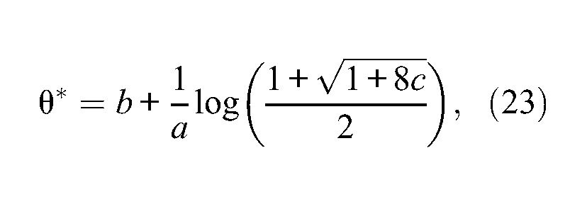
which corresponds exactly to the result provided by Lord (1980). Moreover, under the 2PL model for which c = 0 and d = 1, the item information function given by Equation 7 reduces to $I (x) = a^{2} x (1 - x)$ and is maximized whenever x = 0.5, implying that $θ^{*} = b$ is the optimal ability level. This is a well-known result that can even be inferred from Equation 23 directly.

Illustration

Let us provide a practical illustration. Consider an artificial item with the following parameters: a = 1.1, b = −1, c = 0.2, and d = 0.95. The polynomial p(x) for this item is actually depicted in the aforementioned Figure 1, while the item information function is displayed in Figure 2.

Figure 2.

Item information function for an artificial item with parameters a = 1.1, b = −1, c = 0.2, and d = 0.95.

First,

u = - \frac{3}{4} + \frac{0.2 + 0.95 - 2 \times 0.2 \times 0.95}{2} = - 0.365 and v = \frac{0.2 + 0.95 - 1}{4} = 0.0375,

so that $Δ = 0 . 0375^{2} + 4 \times (- 0.365)^{3} / 27 = - 0.0058$ and is negative, as expected. The three real roots of p(x) are then obtained as follows:

x_{1} = 2 \sqrt{\frac{0.365}{3}} \cos {\frac{1}{3} acos (- \frac{0.0375}{2} \sqrt{\frac{27}{{0.365}^{3}}})} + 0.5 = 1.044,

x_{2} = 2 \sqrt{\frac{0.365}{3}} \cos {\frac{1}{3} acos (- \frac{0.0375}{2} \sqrt{\frac{27}{{0.365}^{3}}}) + \frac{2 π}{3}} + 0.5 = - 0.150,

and

x_{3} = 2 \sqrt{\frac{0.365}{3}} \cos {\frac{1}{3} acos (- \frac{0.0375}{2} \sqrt{\frac{27}{{0.365}^{3}}}) + \frac{4 π}{3}} + 0.5 = 0.606 .

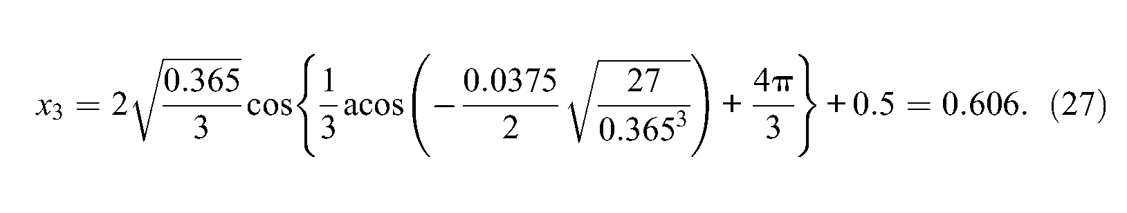
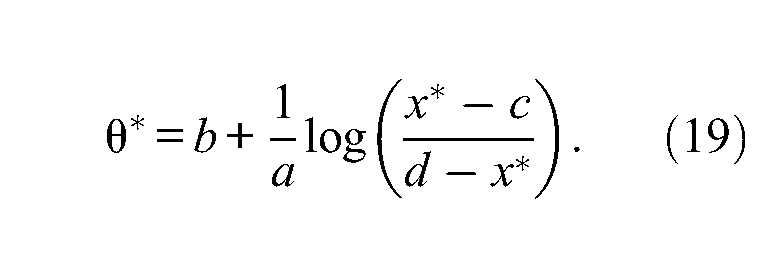
This confirms the previous findings and the expected ordering of the three real roots. These are displayed in Figure 1 by triangles. Finally, using Equation 19, one gets

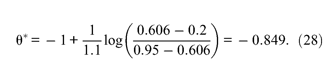
θ^{*} = - 1 + \frac{1}{1.1} \log (\frac{0.606 - 0.2}{0.95 - 0.606}) = - 0.849 .

Hence, the item information function reaches its maximum value whenever θ = −0.849. This optimal value is also represented in Figure 2 and brings a visual confirmation of the accuracy of Equation 19.

Finally, the dependency of $θ^{*}$ on the item parameters was briefly investigated by considering several couples of lower and upper asymptotes, and keeping the item discrimination and difficulty levels fixed to 1 and 0, respectively. The lower asymptote was fixed to 0.0, 0.1, and 0.2 and the upper asymptote to 0.8, 0.9, and 1.0. Table 1 lists, for each of these nine combinations, the corresponding values of u, v, $x^{*} = P (θ^{*})$ , $θ^{*}$ , and $I (θ^{*})$ . These values are routinely returned by the R function displayed in the Appendix. One can notice that both the optimal ability level $θ^{*}$ and the corresponding response probability $P (θ^{*})$ increase with the lower and upper asymptotes, while the maximum information $I (θ^{*})$ decreases.

Table 1.

Values of u, v, $x^{*} = P (θ^{*})$ , $θ^{*}$ , and $I (θ^{*})$ for Nine Combinations of Lower and Upper Asymptote Parameter Values.

c	d	u	v	$x^{} = P (θ^{})$	$θ^{*}$	$I (θ^{*})$
0.0	0.8	−0.35	−0.050	0.347	−0.267	0.170
0.0	0.9	−0.30	−0.025	0.415	−0.158	0.206
0.0	1.0	−0.25	0.000	0.500	0.000	0.250
0.1	0.8	−0.38	−0.025	0.433	−0.095	0.124
0.1	0.9	−0.34	0.000	0.500	0.000	0.160
0.1	1.0	−0.30	0.025	0.585	0.158	0.206
0.2	0.8	−0.41	0.000	0.500	0.000	0.090
0.2	0.9	−0.38	0.025	0.567	0.095	0.124
0.2	1.0	−0.35	0.050	0.653	0.267	0.170

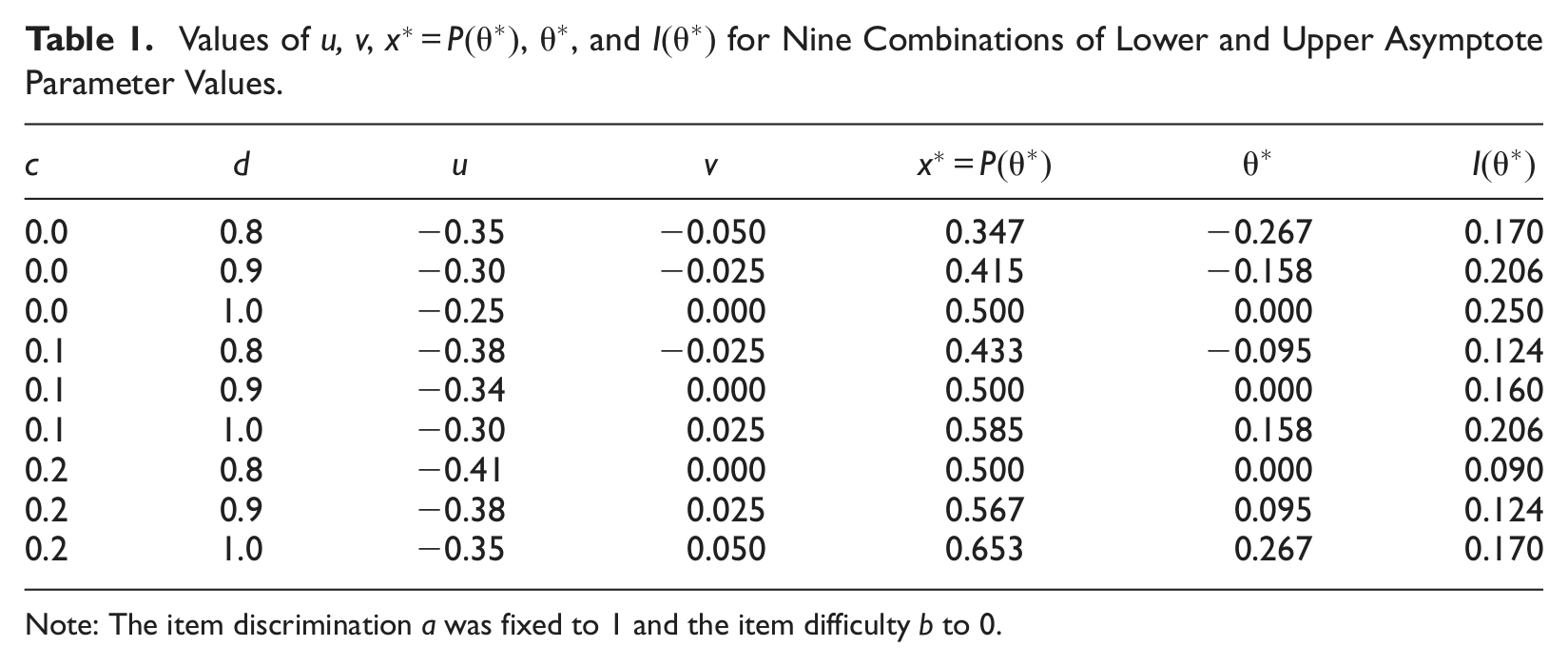
Note: The item discrimination a was fixed to 1 and the item difficulty b to 0.

Final Comments

The purpose of this article was to derive the value of the latent ability level that maximizes the item information function of the 4PL model. The computation is straightforward, and the algebraic formulas 18 and 19 provide the solution to the problem. Note that Equations 19 (for the 4PL model) and 23 (for the 4PL model) are identical, except for the optimal $x^{*}$ value.

Beyond the technical interest of the present study, the developments are most useful when the 4PL model is used in practice. This aspect is probably the most important as there is still a controversy about the usefulness and applicability of the 4PL model for practical purposes. Some such examples were listed earlier in this note. Further motivations are pointed out by Loken and Rulison (2010). It is expected that, besides its technical complexity in getting reliable item parameter estimates, the 4PL model will receive more attention in the years to come.

With respect to the usefulness of the present study under the 4PL model, at least two practical fields of application can be mentioned. The first one is the CAT framework, for which several applications of the 4PL model were mentioned earlier. A more straightforward and practical application of this result is the following. Chang and Yin (2008) characterized the reason why high-ability respondents might get lower scores than expected when answering a CAT and missing the first items of the test. Under this scenario, easy and highly discriminating items will be selected (under the maximum information criterion to select the next item), which breaks down the recovery of the ability estimates toward their true value, unless the test gets longer. In their mathematical derivations, the authors made use of Lord’s (1980) result displayed here in Equation 23. Furthermore, as already pointed out, Rulison and Loken (2009) illustrated how the 4PL model could limit this underestimating trend due to early mistakes in CAT. By setting the upper asymptotes smaller than 1, and thus allowing high-ability respondents to miss the first items with greater probability, one is able to lessen the underestimation at the first steps and thus, to recover quickly from early mistakes. The challenge for explaining this improvement under the 4PL model would then be to extend Chang and Yin’s (2008) discussion to this model. To this end, the present optimal value in Equation 19 will most probably be necessary to understand and characterize this mechanism.

The second potentially interesting field of application is the robust estimation of ability levels (Mislevy & Bock, 1982; Schuster & Yuan, 2011). When response disturbances (such as guessing, cheating, or inattention) interfere with the item response process, the classical estimators can return very biased estimates of ability. Robust alternatives were developed by weighting the log-likelihood function such that aberrant item responses are down-weighted and, consequently, have less impact on the final ability estimate. Although the process is straightforward and relies on an appropriate choice of a weighting function and a residual measure, the current suggested residuals measures rely only on the 2PL model. Recently, Magis (2012) introduced two generalizations of the residual measures that can be handled with any dichotomous item response model. One of the proposed residual measures relies on the maximization of the item information function, by giving maximal weight whenever this item information is maximized. The study discussed in detail the case of the 3PL model, for which Equation 23 is widely available. Under the 4PL model, the present algebraic result given by Equation 19 could also be used similarly, leading eventually to allow robust estimation of ability under the 4PL model with appropriate weights and residuals.

Footnotes

Appendix

Acknowledgements

The author wishes to thank two anonymous reviewers for their helpful comments.

Declaration of Conflicting Interests

The author declared no potential conflicts of interest with respect to the research, authorship, and/or publication of this article.

Funding

The author disclosed receipt of the following financial support for the research, authorship, and/or publication of this article: This research was financially supported by a Research Grant “Chargé de recherches” of the National Funds for Scientific Research (FNRS, Belgium), the IAP Research Network P7/06 of the Belgian State (Belgian Science Policy), and the Research Funds of the KU Leuven, Belgium.

References

Barton

M. A.

Lord

F. M.

(1981). An upper asymptote for the three-parameter logistic item-response model. Princeton, NJ: Educational Testing Service.

Birnbaum

(1968). Some latent trait models and their use in inferring an examinee’s ability. In Lord

F. M.

Novick

M. R.

(Eds.), Statistical theories of mental test scores (pp. 397-479). Reading, MA: Addison-Wesley.

Chang

H.-H.

Yin

(2008). To weight or not to weight? Balancing influence of initial items in adaptive testing. Psychometrika, 73, 441-450.

Green

B. F.

(2011). A comment on early student blunders on computer-based adaptive tests. Applied Psychological Measurement, 35, 165-174.

Hambleton

R. K.

Swaminathan

(1985). Item response theory: Principles and applications. Boston, MA: Kluwer.

Jacobson

(1985). Basic algebra I (2nd ed.). San Francisco, CA: W. H. Freeman.

Liao

W.-W.

R.-G.

Yen

Y.-C.

Cheng

H.-C.

(2012). The four-parameter logistic item response theory model as a robust method of estimating ability despite aberrant responses. Social Behavior and Personality, 40, 1679-1694.

Linacre

J. M.

(2004). Discrimination, guessing and carelessness: Estimating IRT parameters with Rasch. Rasch Measurement Transactions, 18, 959-960.

Loken

Rulison

K. L.

(2010). Estimation of a four-parameter item response theory model. British Journal of Mathematical and Statistical Psychology, 63, 509-525.

10.

Lord

F. M.

(1980). Applications of item response theory to practical testing problems. Hillsdale, NJ: Lawrence Erlbaum.

11.

Lunn

D. J.

Thomas

Best

Spiegelhalter

(2000). WinBUGS—A Bayesian modeling framework: Concepts, structure, and extensibility. Statistics and Computing, 10, 325-337.

12.

Magis

(2012). Some robust ability estimators with logistic item response models. Unpublished manuscript, Department of Education, University of Liège, Liège, Belgium.

13.

Magis

Raîche

(2012). Random generation of response patterns under computerized adaptive testing with the R package catR. Journal of Statistical Software, 48, 1-19.

14.

Mislevy

R. J.

Bock

R. D.

(1982). Biweight estimates of latent ability. Educational and Psychological Measurement, 42, 725-737.

15.

Osgood

McMorris

B. J.

Potenza

M. T.

(2002). Analyzing multiple-item measures of crime and deviance I: Item response theory scaling. Journal of Quantitative Criminology, 18, 267-296.

16.

R Development Core Team. (2012). R: A language and environment for statistical computing [Computer software]. Vienna, Austria: R Foundation for Statistical Computing.

17.

Reise

S. P.

Waller

N. G.

(2003). How many IRT parameters does it take to model psychopathology items?Psychological Methods, 8, 164-184.

18.

Rulison

K. L.

Loken

(2009). I’ve fallen and I can’t get up: Can high ability students recover from early mistakes in computerized adaptive testing?Applied Psychological Measurement, 33, 83-101.

19.

Rupp

A. A.

(2003). Item response modeling with BILOG-MG and MULTILOG for Windows. International Journal of Testing, 3, 365-384.

20.

Schuster

Yuan

K.-H.

(2011). Robust estimation of latent ability in item response models. Journal of Educational and Behavioral Statistics, 36, 720-735.

21.

Tavares

H. R.

de Andrade

D. F.

Pereira

C. A.

(2004). Detection of determinant genes and diagnostic via item response theory. Genetics and Molecular Biology, 27, 679-685.

22.

Tendeiro

J. N.

Meijer

R. R.

(2012). A CUSUM to detect person misfit: A discussion and some alternatives for existing procedures. Applied Psychological Measurement, 36, 420-442.

23.

Waller

N. G.

Reise

S. P.

(2009). Measuring psychopathology with non-standard IRT models: Fitting the four parameter model to the MMPI. In Embretson

Roberts

J. S.

(Eds.), New directions in psychological measurement with model-based approaches (pp. 147-173). Washington, DC: American Psychological Association.

24.

Yen

Y.-C.

R.-G.

Liao

W.-W.

Chen

L.-J.

Kuo

C.-C.

(2012). An empirical evaluation of the slip correction in the four parameter logistic models with computerized adaptive testing. Applied Psychological Measurement, 36, 75-87.