Modeling Pacing Behavior and Test Speededness Using Latent Growth Curve Models

Purpose

The present study illustrates, for the first time, how a longitudinal multilevel modeling approach can be used to evaluate pacing behavior and so enhance the study of test speededness. More specifically, a confirmatory modeling approach based on an SEM framework is used to explore the usefulness of latent growth curve modeling in detecting both within- and between-person differences in examinee pacing behavior. The proposed methodology is applied to data from a high-stakes computerized examination that was subjected to a timing change. The following questions were of interest: How does item response time change as a function of item presentation order? How much individual variability is there around the overall rate of change across item presentation orders? If significant differences in individual rates of change exist, does native language explain this variance? Does the influence of native language on response time vary as a function of examinee proficiency? and, finally, Did the pacing behavior of examinees differ between the pre- and post–timing change conditions?

Method

Data

Study data included item responses and response times for examinees who completed a high-stakes, computerized, multiple-choice examination either the year before or the year after the exam was subjected to a timing change where the number of test items was decreased allowing examinees more time per item. The application presented uses data from one of the eight separately timed hour-long test blocks of the examination, including 49 items pre- and 45 items post-timing change.

The sample included 46,701 examinees, of which 23,471 tested during the pre-timing change year and 23,230 tested during the post-timing change year. Approximately one third of the sample spoke English as a second language. The order of items within test blocks was completely randomized across examinees. Randomization of item presentation orders is a common practice for many computer-delivered examinations and aims at enhancing test security as well as controlling potentially confounding effects of item characteristics, such as word count or item difficulty (e.g., Leary & Dorans, 1985; Meyers, Miller, & Way, 2008). Through randomization, it can be assumed that the nominal presentation order substantially accounts for examinees’ actual behavior in completing the examination and that the measure of the dependent variable (response time) is the same at all occasions (item presentation orders) with any differences being attributable to time.

Panels a and b in Figure 1 show observed response times across the test span of the pre- and post-timing change conditions, respectively. Pacing patterns of examinees appear to be distinct for nonnative and native English speakers, but not necessarily for pre- and post-timing change examinees. Even though post-timing change response times were greater than those of the pre-timing change, it appears that having more time did not substantially affect the extent to which examinees had to speed up toward the end of the examination. Post-timing change examinees spent approximately five additional seconds on items presented early in the examination as compared with those presented later. Figure 1 reveals that examinees from both timing conditions spent more time on items presented earlier in the test and increased their pace as they moved through the test and had a slightly smaller change in pacing over the course of the examination if their native language was English.

OPEN IN VIEWER

Figure 1.

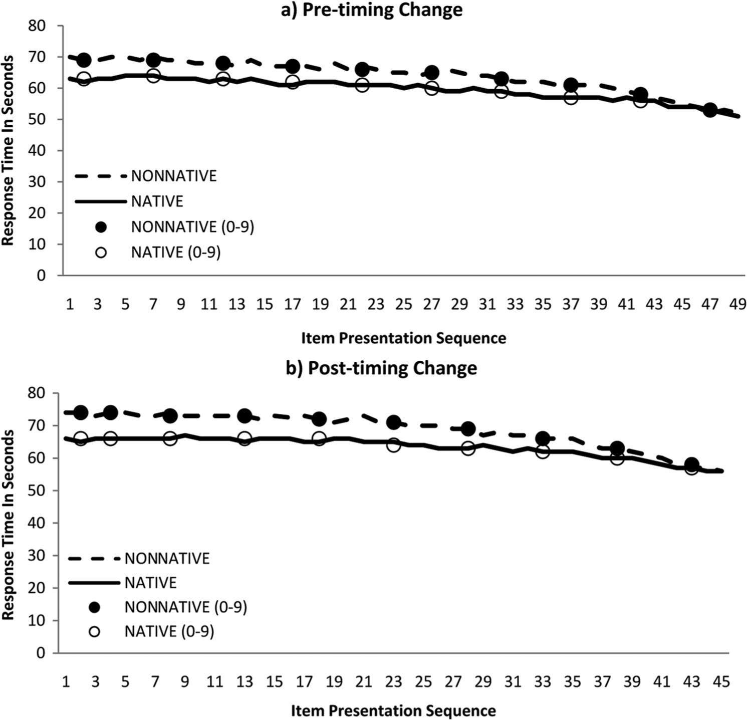
Pre- and post-timing change median response times by native language.

Modeling

To simplify the modeling process and interpretation of results, original item individual presentation orders (time points) were grouped into a smaller number of item presentation order intervals (time intervals). Although this practice of merging a few consecutive measurement occasions into intervals to obtain a time scale with less time points is clearly optional to the execution of the methodology, the authors believe that it may help simplify the modeling process for longer tests with low risk of speededness. Nonetheless, we suggest that practitioners take precautions not to dismiss useful information while attempting to simplify the modeling process.

For the present study with more than 40 item presentation sequences both pre- and post-timing change, the authors experimented with 5-, 10-, 15- and 20-point time-interval scales. A 10-point time-interval scale closely approximated those observed without any categorization and was selected for model building. Note that the number of items presented in each time interval necessarily differs across the two timing conditions. To allow the most optimal comparison, the authors preferred to make the initial rather than the later time intervals of the post-timing change test shorter.

For the pre-timing change condition with a total of 49 items, Time Interval 0 included four item presentation sequences (1st to 4th), whereas the following Time Intervals 1 through 9 each included five item presentation sequences. For the post-timing change with a total of 45 items, Time Interval 0 included two item presentation sequences (1st and 2nd), Time Interval 2 included the next three item sequences (6th to 8th), and the remaining time intervals each included the next five items. Figure 1 plots median response times (plotted as circles) corresponding to item presentation sequence intervals and shows that the 10-point time-interval scale parsimoniously captures how the speed with which examinees work through presented items increases toward the end of the examination. In the figure, it can be seen that even the median response times observed for the first two time intervals in the post-timing change (with less time points) provide a very close approximation to response times observed for the corresponding time points. This was anticipated for there is very little change in response speed for first few time points.

Formulating a Series of Alternative Growth Curve Models

A series of latent growth curve models was fit to the data for each pre- and post-timing change condition to evaluate (a) item response time trajectories, (b) variability around the initial status and overall rate of change, (c) the influence of native language and overall proficiency on the trajectories and on the variance around the trajectories, and (d) if examinee pacing changed post-timing change as represented by changes in (a), (b), and (c). In this context, item presentation order refers to the 10 time intervals (coded 0-9) created from the order in which individual items were presented during the examination. It was assumed that most examinees started from the first item presented and worked their way through the examination to the last item presented, although the test delivery software did not enforce this sequence. Although this approach oversimplifies the data structure by ignoring item features other than presentation order, it has two advantages. First, it allows various comparisons to be made about whether examinees spent more time on items presented in the beginning, middle, or at the end of a test session without any specific references to particular test items. Second, it allows form-free summaries to be meaningful as item presentation sequences are completely randomized within test forms.

The first modeling task involved identifying the appropriate form of the relationship between presentation order and item response times. Visual representations of the data were used in formulating a couple of alternative models which were then tested to select the base model with the best fit statistics. This was followed by formulating the following four models each built by adding one or two predictor variables to the base model: (a) a multigroup model with native language as a group variable, (b) a multigroup model with native language as a group variable and examinee proficiency as a time-varying covariate, (c) a single-group model with native language as a covariate, and (d) a single-group model with native language, proficiency, and a language-by-proficiency interaction term as covariates. Table 1 describes the four models.

OPEN IN VIEWER

Table 1.

Estimated Three-Piece Linear Growth Curve Models With One or Two Predictors.

Model	Type	Description	Predictors
			Native language	Proficiency a	Native language-by-proficiency interaction b
Model 1	Reduced	A multigroup model with no covariates	As a group variable	—	—
Model 2	Full	A multigroup variable with a time-varying covariate	As a group variable	As a time-varying covariate	—
Model 3	Reduced	A single-group model with a time-invariant covariate	As a time-invariant covariate	—	—
Model 4	Full	A single-group model with time-invariant covariates	As a time-invariant covariate	As a time-invariant covariate	As a time-invariant covariate

a

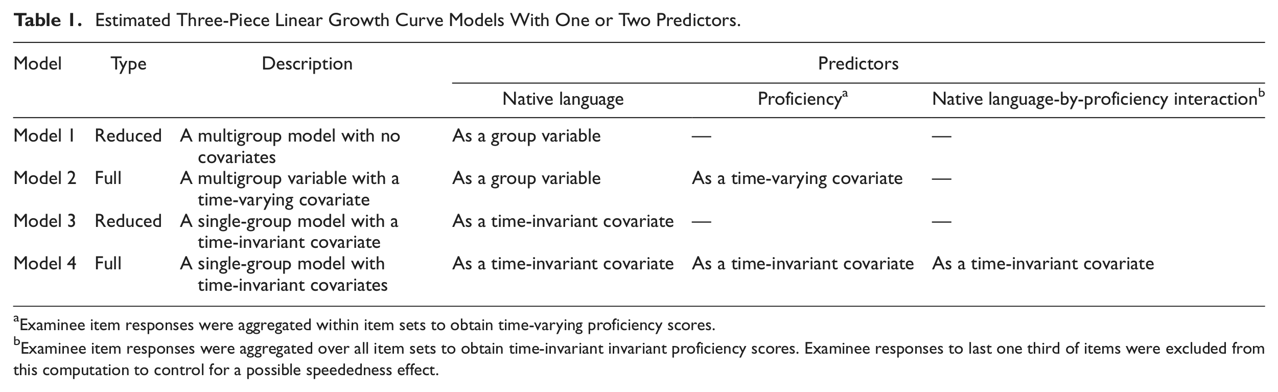
Examinee item responses were aggregated within item sets to obtain time-varying proficiency scores.

b

Examinee item responses were aggregated over all item sets to obtain time-invariant invariant proficiency scores. Examinee responses to last one third of items were excluded from this computation to control for a possible speededness effect.

The rationale for selecting these models is as follows. Detecting potential differences in examinees pacing patterns is a focal point of test speededness research. Clearly, models that can incorporate group variables have great potential for aiding empirical investigations of pacing behavior for examinees from distinct subpopulations. Model 1 is a reduced two-group model estimated to test whether estimated parameters reflecting change over time (t = 0-9) were different for native and nonnative English speakers. If group differences exist, a logical next step would be to investigate whether examinee proficiency explained some of the variance. Model 2 is the full two-group model with proficiency as a time-varying covariate. It examined the influence of proficiency on response time trajectories for the two language groups and investigated whether there were any language-by-proficiency interaction effects over time intervals. Time-varying proficiency scores used in Model 2 were computed as an average item response score for each examinee on each time interval (producing a total of 10 time-interval scores per examinee.) Any increase in goodness of fit for Model 2, the full model, compared with Model 1, the reduced model, can be attributed to the addition of the time-varying proficiency covariate.

Models 3 and 4 were formed as alternatives to Models 1 and 2 using a similar rationale. Model 3 uses native language as a time-invariant covariate and serves as a reduced model while Model 4, the full model, extents it by incorporating a proficiency covariate. The difference is that these models are single-group models that use a native language group variable as a covariate rather than a multigroup variable. Entering a group variable into a growth curve model as a covariate is analogous to entering a dichotomous variable into a regression model which is accomplished by dummy coding the group variable. The disadvantage of this strategy is that the resulting intercepts and slope estimates in this model will be group contrasts rather than group-specific values. The advantage, however, is that, as in Model 4, both covariates can be entered as Level 2 predictors allowing a language-by-proficiency interaction effect to be tested along with language and proficiency main effects. Therefore, formulating Model 4, the authors were able to test the influence of proficiency on response time trajectories for the two language groups and whether there were any language-by-proficiency interaction effects over time. Proficiency in this model is a time-invariant covariate and was computed as an average score per examinee. To control for the influence of speededness on proficiency scores, items presented during the last one third of the examination were excluded from the average score computation. Any increase in goodness-of-fit for Model 4, the full model, compared with Model 3, the reduced model, can be attributed to the addition of the proficiency and language-by-proficiency time-invariant covariates.

All four models were fit to test data from the pre- and post-timing change administrations. The log transformation was used to normalize response time distributions for model estimation. The different models were estimated with Mplus (Muthén, 2004) using the maximum likelihood estimator. Consistent with recommended practices (see Hu & Bentler, 1999; McDonald & Ho, 2002, for a detailed discussion), more than one fit index was used in evaluating model fit. The models were compared using (a) the Bentler Comparative Fit Index (CFI; Bentler, 1990), where values greater than 0.95 indicate a good model fit; (b) the root mean square error of approximation (RMSEA), where values smaller than 0.05 indicate a good model fit; (c) the negative log likelihood; and (d) the Bayesian Information Criterion (BIC). For these latter two indices, smaller values indicate a better fit and are often used to test goodness-of-fit for a full model in comparison with a reduced one.

Identifying the Appropriate Growth Curve Form

Initial analyses were conducted to identify the appropriate growth curve form which would accurately and parsimoniously describe the downward trend in the amount of time examinees spent on items as a function of presentation order. Preliminary analyses of the data indicated that a linear model would be inappropriate as the downward turn in response times was gradual at the initial time intervals and gained momentum toward the final time intervals. Relying on the observed change over time (see Figure 1), a quadratic model was considered first. The quadratic latent growth curve model was estimated by Equation 1:

Level 1 y it = η 0 i + η 1 i a it + η 2 i a it 2 + ε it ,

η 0 i = β 0 + ζ 0 i ,

Level 2 η 1 i = β 1 + ζ 1 i ,

η 2 i = β 2 + ζ 2 i ,

where t represents the item set coded 0 to 9, i represents the examinee (i = 1, 2, . . . , N), y represents the log response time influenced by the random effects η_0i, η_1i, and η_2i representing the intercept, a linear term, and a quadratic term, respectively. The intercept, η_0i, describes an examinee’s initial log response time when starting the examination. The linear term, η_1i, describes the rate of change in log response time over the course of the examination, with positive values indicating growth and negative values indicating decline. The quadratic term, η_2i, describes the rate of acceleration in the rate of change over the course of the examination.

A piecewise latent growth curve model was considered next. A careful inspection of Figure 1 reveals that the downward trend in speed might be occurring in three distinct stages. In the first phase, examinees appear to move at a relatively slow pace and there is not much decline in response times. In the second phase, examinees are somewhat faster, but, no drastic changes in their speed occur. In the final stage, which corresponds to the end of the examination, examinees moved from one item to another at a faster rate. The best fit was achieved for the three-piece model that used the first three, the middle four, and the last three item sets as three phases of change. Equation 2 shows the model:

Level 1 y it = η 0 i + η 1 i a 1 it + η 2 i a 2 it + η 3 i a 3 it + ε it , η 0 i = β 0 + ζ 0 i , Level 2 η 1 i = β 1 + ζ 1 i , η 2 i = β 2 + ζ 3 i , η 3 i = β 3 + ζ 3 i ,

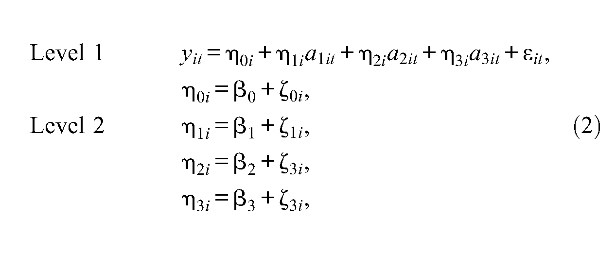
where η₀ represents the intercept, and η₁, η₂, and η₃ represent the first, second, and third linear terms for the beginning, middle, and final phases of change, respectively.

Table 2 lists the CFI and RMSE statistics for the quadratic and three-piece models and suggests that the three-piece model fits the data either equally well or better than the quadratic model for both pre- (T1) and post-timing change (T2) conditions. (Negative log likelihood and BIC fit indices are also provided even though these two, being relative model fit indices, are not considered very meaningful when comparing models that are not nested.) Providing a visual aid, Figure 2 plots observed and estimated log response times from both the quadratic and three-piece models. (The figure also includes a time interval by phase list for the three-piece model.) The figure reveals that the quadratic effects of time provide a good representation of initial changes in response speed but tend to depart markedly from the observed in the second and third phases. The three-piece model appears to approximate the downward trend in response times better than the quadratic model for both time conditions. Relying on these results, the linear piecewise model with three phases of change was used for further model building.

OPEN IN VIEWER

Table 2.

Model Fit Comparisons Over Test Blocks Pre- (T1) and Post-Timing Change (T2).

		T1				T2
Model		CFI	NLogL	BIC	RMSEA	CFI	NLogL	BIC	RMSEA
M0	Quadratic	0.960	22,461	45,204	0.021	0.959	37,665	75,591	0.022
M0	PW3 a	0.964	21,840	44,023	0.018	0.963	36,978	74,298	0.021
M1	PW3 LAN b MG c	0.959	19,665	39,814	0.018	0.927	34,274	69,031	0.024
M2	PW3 LAN MG with PROF d	0.938	12,628	25,941	0.021	0.935	27,640	55,964	0.021
M3	PW3 LAN	0.970	20,632	41,545	0.016	0.955	35,387	71,056	0.021
M4	PW3 LAN, PROF, LAN × PROF e	0.973	20,084	40,510	0.014	0.959	34,751	69,843	0.018

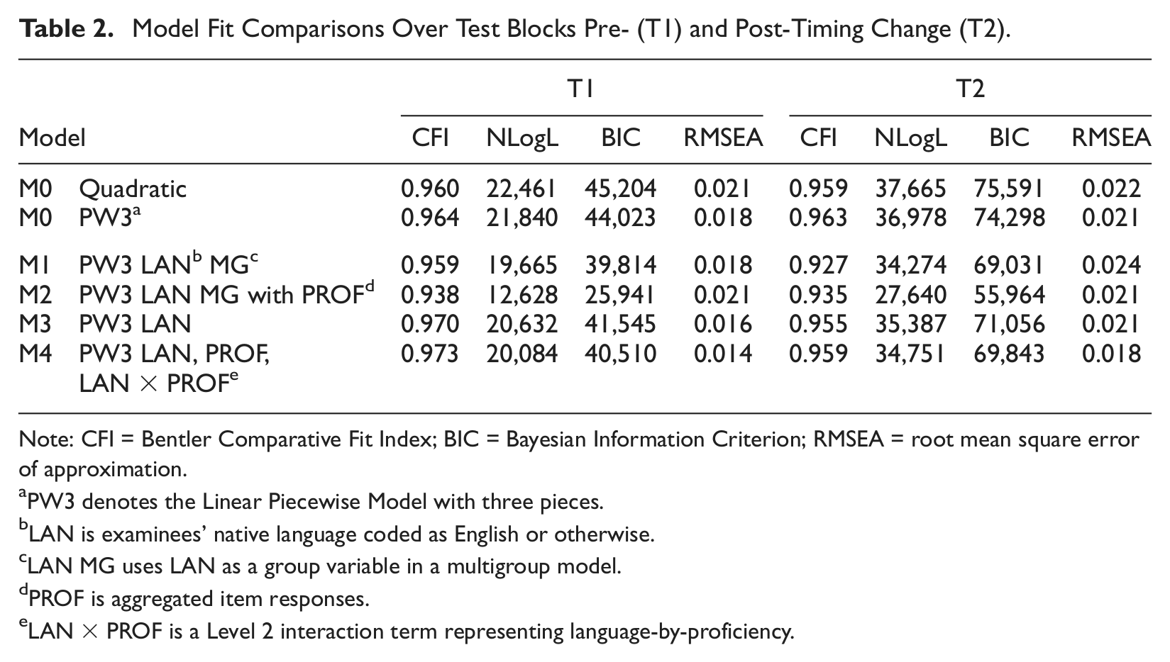
Note: CFI = Bentler Comparative Fit Index; BIC = Bayesian Information Criterion; RMSEA = root mean square error of approximation.

a

PW3 denotes the Linear Piecewise Model with three pieces.

b

LAN is examinees’ native language coded as English or otherwise.

c

LAN MG uses LAN as a group variable in a multigroup model.

d

PROF is aggregated item responses.

e

LAN × PROF is a Level 2 interaction term representing language-by-proficiency.

OPEN IN VIEWER

Figure 2.

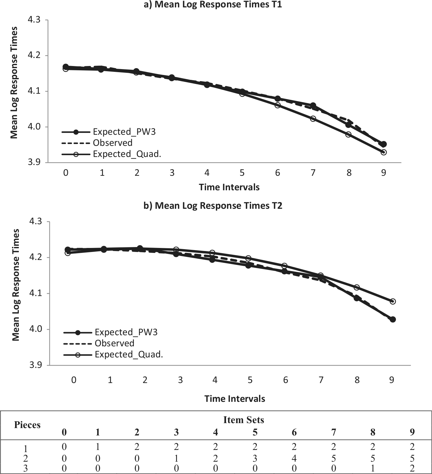
Observed and expected quadratic (quad.) and three-piece linear (PW3) log response times for pre- (T1) and post-timing change (T2).

Predicting Response Times With Multigroup Models: Models 1 and 2

The three-piece multigroup models were estimated by Equation 3:

Level 1 y git = η g 0 i + η 1 i a 1 it + η 2 i a 2 it + η 3 a 3 it + κ it x it + ε it , η ESL 0 i = β ESL 0 + ζ ESL 0 i , Level 2 a η ESL 1 i = β ESL 1 + ζ ESL 1 i , η ESL 2 i = β ESL 2 + ζ ESL 2 i , η ESL 3 i = β ESL 3 + ζ ESL 3 i , η ENL 0 i = β ENL 0 + ζ ENL 0 i ,

Level 2 b η ENL 1 i = β ENL 1 + ζ ENL 1 i , η ENL 2 i = β ENL 2 + ζ ENL 2 i , η ENL 3 i = β ENL 3 + ζ ENL 3 i ,

where ENL represents examinees who speak English as a native language, ESL represents examinees who speak English as a second language, x_it represents the time-varying “response accuracy” covariate for examinee i where coefficients κ _it , η₀, η₁, η₂, and η₃ represent the group-specific intercept and three linear slopes for the beginning, middle, and final phases of change, respectively. x_it was dropped from the equation when estimating the reduced multigroup model, Model 1. Note that in latent growth curve modeling, the slopes of time-varying covariates are estimated using the within-person model and vary over time points.

Predicting Response Times With Single-Group Models: Models 3 and 4

The three-piece single-group models were estimated by Equation 4:

Level 1 y it = η 0 i + η 1 i a 1 it + η 2 i a 2 it + η 3 a 3 it + ε it , η 0 i = β 0 + γ 10 g i 0 + γ 20 x i 0 + γ 30 g x i 0 + ζ 0 i , Level 2 η 1 i = β 1 + γ 11 g i 0 + γ 21 x i 0 + γ 31 g x i 0 + ζ 1 i , η 2 i = β 2 + γ 12 g i 0 + γ 22 x i 0 + γ 32 g x i 0 + ζ 2 i , η 3 i = β 3 + γ 13 g i 0 + γ 23 x i 0 + γ 33 g x i 0 + ζ 3 i ,

g = { 0 if the examinee spoke English as a second language , ESL 1 if the examinee spoke English as a native language , ENL

where x₀ represents examinee proficiency computed from item responses and gx₀ represents the language-by-proficiency interaction term. x₀ and gx₀ were dropped from the equation when estimating the reduced single-group model, Model 3. In Model 4, the interaction term was not significantly related to the slopes for the beginning and middle phases and was removed from the model.

Results

Table 2 lists model fit statistics for all four 3-piece models for pre- and post-timing change conditions. Overall, the results suggest that the goodness-of-fit observed for the four models range from acceptable to very good. Relative model fit indices suggest that Models 2 and 4, the full models, fit the data better than their reduced counterparts, Models 1 and 3. The model with the consistently best fit, however, was Model 4, which used native language, proficiency, and the interaction of the two as between-person covariates.

Table 3 shows the group-specific random coefficients (intercepts and slopes) produced by Model 1 for the two timing conditions. These results suggest that in both timing conditions, native and nonnative English speakers differed in two respects: in the estimates of their initial status (intercepts) and their rates of change during the final phase of the examination (slopes). Nonnative English speakers were estimated to spend approximately 4 s more answering items. For both groups, the final slopes were drastically larger than the beginning or middle slopes, confirming that there was a negative downward trend in log response times toward the end of the examination. This pattern was slightly more pronounced for nonnative English speakers. The differences in the variances around the intercepts were very small, even though nonnative English speakers appeared to have slightly larger variances. The estimated variances around the slopes were much larger for the final slopes, especially for nonnative English speakers.

OPEN IN VIEWER

Table 3.

Model 1 Parameter Estimates for Test Blocks Pre- (T1) and Post-Timing Change (T2).

		T1				T2
		Random coefficients (SE)				Random coefficients (SE)
LAN a	Statistics	Intercept	S1	S2	S3	Intercept	S1	S2	S3
NNAT b	M	4.223 (0.003)	−0.007 (0.002)	−0.022 (0.001)	−0.079 (0.002)	4.285 (0.004)	0.000 (0.002)	−0.019 (0.001)	−0.083 (0.002)
	Variance	0.012 (0.002)	0.003 (0.001)	0.001 (0.001)	0.020 (0.001)	0.020 (0.003)	0.005 (0.001)	0.001 (0.001)	0.021 (0.002)
NAT c	M	4.143 (0.002)	−0.006 (0.001)	−0.018 (0.001)	−0.043 (0.001)	4.187 (0.003)	0.003 (0.002)	−0.014 (0.001)	−0.045 (0.002)
	Variance	0.016 (0.001)	0.002 (0.001)	0.001 (0.001)	0.009 (0.001)	0.018 (0.002)	0.002 (0.001)	0.001 (0.001)	0.009 (0.001)

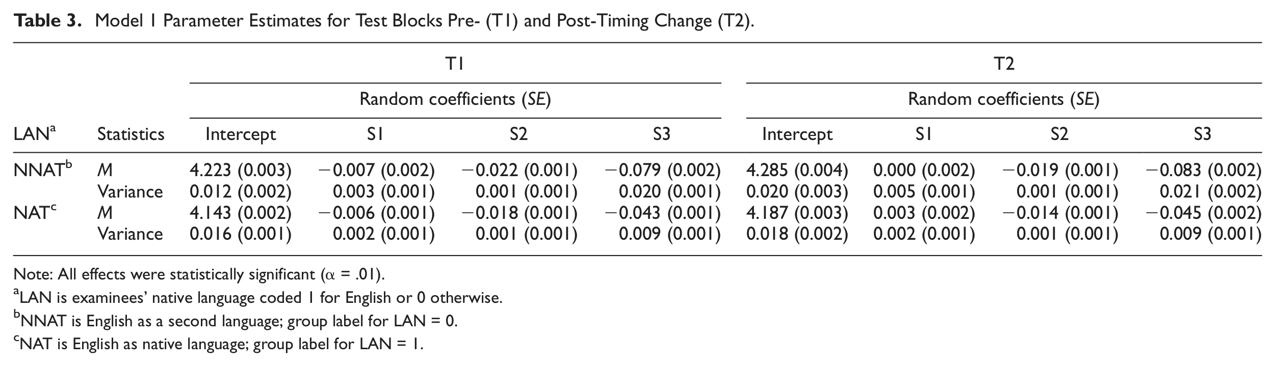
Note: All effects were statistically significant (α = .01).

a

LAN is examinees’ native language coded 1 for English or 0 otherwise.

b

NNAT is English as a second language; group label for LAN = 0.

c

NAT is English as native language; group label for LAN = 1.

Before the timing change, native English speakers started an item block spending approximately 3 to 4 s less per item; they also exhibited 50% more slowly declining rates than nonnative English speakers. The variability across examinees unaccounted for by item set presentation sequence (i.e., residual variability) ranged from 0 to 0.20 for the estimates of the intercepts and final slopes and was slightly larger for nonnative English speakers. This pattern remained after the timing change except that the gap between native and nonnative English speakers widened by 1 s. Figure 3 plots group-specific intercept and final slope estimates for the two timing conditions. This figure shows that examinees who took the examination after the timing change had an initial advantage over those who took the examination before the timing change (larger intercepts), but without any lasting effects. Examinees, given their language group, ran out of time in a similar manner in both timing conditions (i.e., the slopes were very similar).

OPEN IN VIEWER

Figure 3.

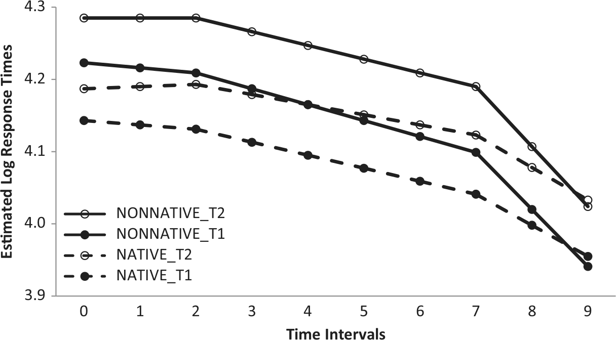
Model 1 estimated item log response times for nonnative and native language groups pre- (T1) and post-timing change (T2).

Table 4 presents the group-specific intercept and slope parameters produced by Model 2. As reflected by the lack of additional improvement in model fit for Model 2, the negative relationship between proficiency and response time was rather weak. Although Model 2 was not the best fitting model, it provided useful information about how response accuracy relates to log response times observed for the two language groups. Figure 4 plots within-person response accuracy slopes estimated by Model 2 and illustrates how latent growth curve modeling can help track how the rate of change in response times differs within a person over the course of the examination. The figure shows that the estimated proficiency coefficients averaged approximately −0.27 for native English speakers and −0.33 for nonnative English speakers during the first seven time intervals without much fluctuation, but with a decline during Time Intervals 8 and 9. It also shows that the drop off observed in the last phase was faster for nonnative English speakers when compared with native English speakers. This indicates that there was a language-by-proficiency interaction in the last phase.

OPEN IN VIEWER

Table 4.

Model 2 Parameter Estimates for Test Blocks Pre- (T1) and Post-Timing Change (T2).

LAN a	Statistics	Random coefficients (SE)				Time-variant PROF b coefficients (SE)
		Intercept	S1	S2	S3	Time	0	1	2	3	4	5	6	7	8	9
T1
NNAT c	M	4.397 (0.008)	0.001 (0.005)	−0.026 (0.002)	−0.177 (0.007)	NNAT	−0.254 (0.011)	−0.257 (0.007)	−0.280 (0.009)	−0.270 (0.007)	−0.250 (0.006)	−0.248 (0.006)	−0.254 (0.007)	−0.262 (0.009)	−0.089 (0.008)	0.026 (0.015)
	Variance	0.012 (0.001)	0.003 (0.001)	0.001 (0.001)	0.019 (0.001)
NAT d	M	4.375 (0.007)	0.002 (0.004)	−0.022 (0.002)	−0.110 (0.005)	NAT	−0.326 (0.009)	−0.320 (0.006)	−0.344 (0.007)	−0.336 (0.005)	−0.327 (0.005)	−0.324 (0.005)	−0.317 (0.005)	−0.322 (0.007)	−0.212 (0.006)	−0.138 (0.010)
	Variance	0.016 (0.001)	0.002 (0.001)	0.001 (0.001)	0.009 (0.001)
T2
NNAT	M	4.477 (0.009)	0.003 (0.006)	−0.023 (0.002)	−0.199 (0.006)	NNAT	−0.265 (0.011)	−0.284 (0.007)	−0.288 (0.008)	−0.269 (0.007)	−0.251 (0.006)	−0.247 (0.006)	−0.256 (0.007)	−0.268 (0.008)	−0.085 (0.008)	0.074 (0.014)
	Variance	0.021 (0.003)	0.005 (0.001)	0.001 (0.001)	0.019 (0.001)
NAT	M	4.423 (0.007)	0.012 (0.005)	−0.016 (0.002)	−0.122 (0.005)	NAT	−0.319 (0.009)	−0.327 (0.006)	−0.347 (0.007)	−0.334 (0.006)	−0.325 (0.005)	−0.327 (0.005)	−0.334 (0.006)	−0.336 (0.007)	−0.223 (0.006)	−0.126 (0.011)
	Variance	0.020 (0.002)	0.002 (0.001)	0.001 (0.001)	0.009 (0.001)

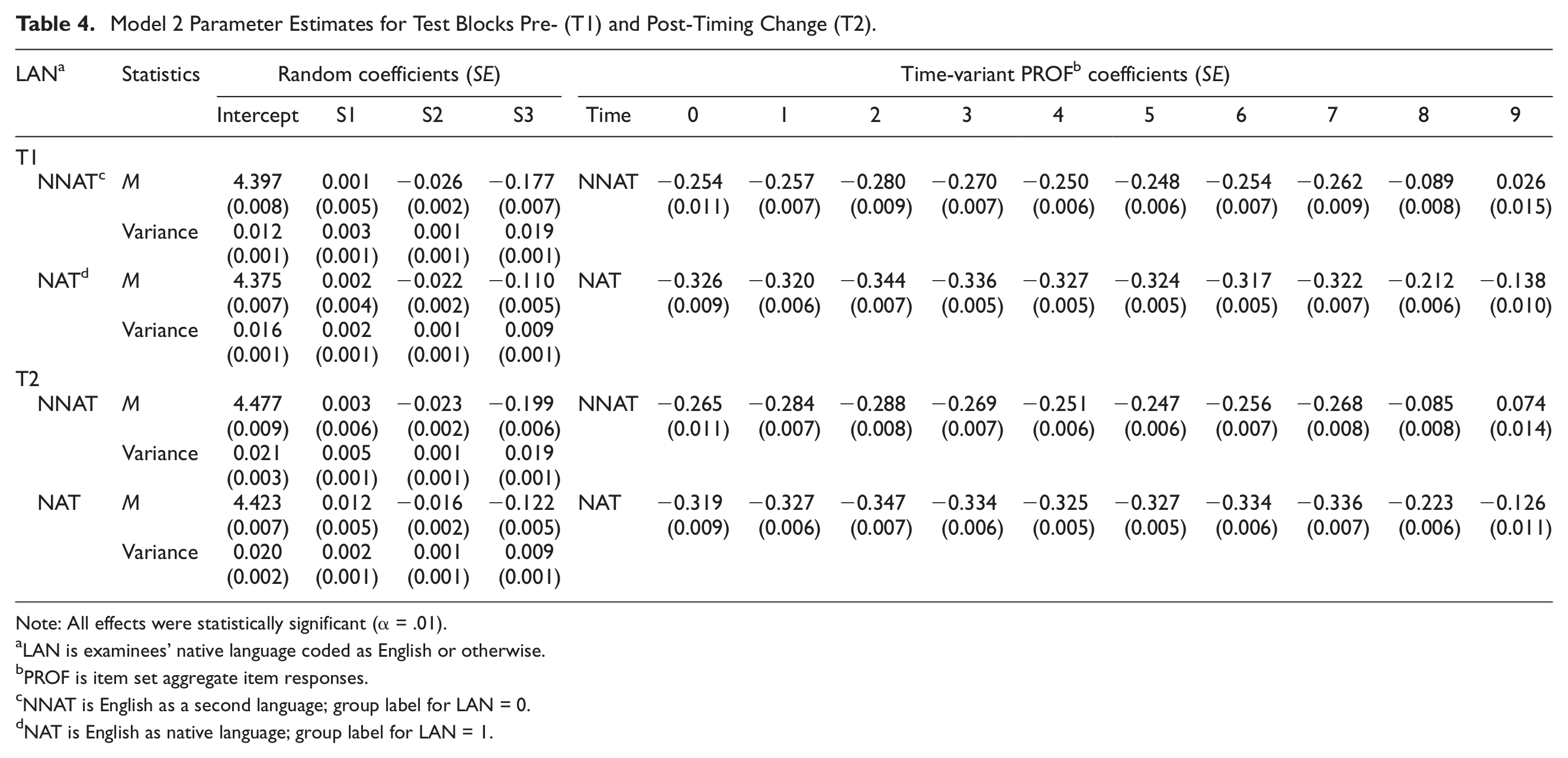
Note: All effects were statistically significant (α = .01).

a

LAN is examinees’ native language coded as English or otherwise.

b

PROF is item set aggregate item responses.

c

NNAT is English as a second language; group label for LAN = 0.

d

NAT is English as native language; group label for LAN = 1.

OPEN IN VIEWER

Figure 4.

Model 2 produced proficiency slopes for nonnative and native language groups pre- (T1) and post-timing change (T2).

The interesting finding was not that the relationship between proficiency and response times was weak, as similar findings are often reported in the response time literature (e.g., Henderson, 2004), but that this relationship changed from the beginning to the end of the test block. Group-specific changes in the relationship between proficiency and response times and a phase-specific interaction effect would have gone unnoticed if a longitudinal perspective had not been used. As such, both multigroup models were useful in capturing within- as well as between-person changes in response times and their relationships to predictor variables.

Table 5 lists the parameters estimated by Model 4, the full single-group model with native language, proficiency, and language-by-proficiency interaction effects. The effect of proficiency was not as prominent as the effect of language, and the effect of the language-by-proficiency interaction term was small. However, when significant language-by-proficiency interaction effects on the intercepts and the final slopes remained in the model, the model fit improved consistently for both timing conditions, making Model 4 the best-fitting model. The variances around the intercepts were small. The variances around the slopes were somewhat larger for the final slope estimates, indicating that there were larger individual differences in the final slopes than in the beginning or middle slopes.

OPEN IN VIEWER

Table 5.

Model 4 Parameter Estimates for Test Blocks Pre- (T1) and Post-Timing Change (T2).

Variable	T1				T2
	Intercept	S1	S2	S3	Intercept	S1	S2	S3
Log response times
M	4.218 (0.003)	−0.008 (0.002)	−0.021 (0.001)	−0.074 (0.001)	4.279 (0.004)	−0.001 (0.002)	−0.018 (0.001)	−0.076 (0.002)
Variance	0.014 (0.001)	0.002 (0.001)	0.002 (0.001)	0.012 (0.001)	0.018 (0.002)	0.003 (0.001)	0.001 (0.001)	0.013 (0.001)
LAN a	−0.072 (0.004)	0.003 (0.002)	0.002 (0.001)	0.030 (0.003)	−0.087 (0.005)	0.005 (0.003)	0.003 (0.001)	0.029 (0.003)
PROF b	−0.022 (0.002)	−0.004 (0.001)	0.004 (0.001)	0.022 (0.002)	−0.025 (0.003)	−0.004 (0.001)	0.004 (0.001)	0.027 (0.002)
LAN × PROF c	−0.008 (0.002)			−0.005 (0.002)	−0.011 (0.002)			−0.010 (0.002)

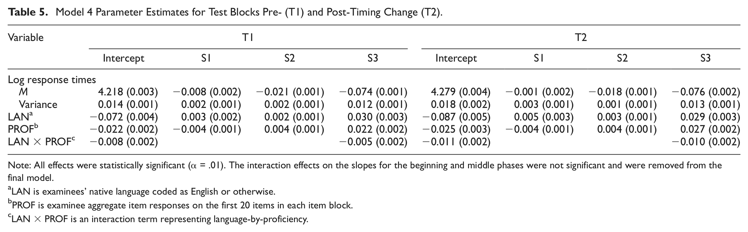
Note: All effects were statistically significant (α = .01). The interaction effects on the slopes for the beginning and middle phases were not significant and were removed from the final model.

a

LAN is examinees’ native language coded as English or otherwise.

b

PROF is examinee aggregate item responses on the first 20 items in each item block.

c

LAN × PROF is an interaction term representing language-by-proficiency.

Overall, the results suggest that both the initial status and the rate of change in response times were subject to within- and between-person differences. Estimated within-person differences in response speed pointed to a triphasic pattern of change over time (or three serial trends each with a speed shift). Examinees from both timing conditions had larger between- and within-person variances for initial response times (intercepts) and the final phase rate of change (final slopes). Estimated between-person differences point to the influence of examinees’ native language as an important predictor. As expected, examinees appear to show greater change in pacing as they move through the test block if they spoke English as a second language. The main effect of this group variable on the intercepts and the final slopes, however, was confounded by a small, yet significant, language-by-proficiency interaction implying that the expected advantage of being a native English speaker was reversed for high- and low-proficiency examinees when they started the examination and when they started to run out of time.

Interestingly, observed within- and between-person differences, as well as the influence of predictor variables on these differences remained almost the same before and after the timing change. Even though examinees improved their pacing skills minimally each time they moved to the next block, the results were comparable for all eight separately timed test blocks of the examination.

Response accuracy rates per time interval were evaluated to investigate the impact of the timing change on observed scores. Within timing conditions, proportion correct scores were 0.03 to 0.04 higher for native English speakers when compared with those for nonnative English speakers. Although a closer look at group-specific gains suggest that native English speakers benefited slightly more from the timing change than nonnative English speakers, differences observed in proportion correct scores were at most 0.02. This increase was constant across time-interval presentation orders and was not detectable in reported test scores due to an adjustment that was made to keep the old and new scores on the same scale.

Discussion

One of the earliest applications of multilevel modeling to predict test speededness was conducted by Bergstrom et al. (1994). Their study used a conventional HLM approach to identify items with characteristics that tended to make them more time-consuming. Harder items, longer items, wrong answers, and those coded as presented in the beginning of the test took longer to complete. Swanson, Case, Ripkey, Clauser, and Holtman (2001) published a similar HLM application and reported similar and some additional interesting findings related to the relationships between examinee proficiency, item difficulty, and response time. In general, examinees with higher proficiencies responded more quickly to items. However, more proficient examinees responded more quickly to easy items and spent more time on hard items.

Although useful for quantifying the characteristics that make items more time-consuming, one limitation with this type of modeling is that these inferences are useful for groups, but not for individuals. Modeling change as a constant rather than a continuous process may conceal within-person differences in speed (i.e., differences in response speed for the beginning, middle, and ending phases of an examination). The present application exemplifies how the impact of a timing change might not be adequately evaluated without a longitudinal model.

The results of the present study suggest that growth curve modeling has added utility because it models change as a continuous process. Modeling within-person differences in pacing may reveal that examinees go through multiple distinct phases of change when working through a block of test items. In the present application, for example, three distinct phases of pacing were identified. The first phase lasted for less than one third of the total test block time. In this phase, examinees moved at a relatively slow pace, and there was little decline in response times. In the second phase, the longest phase, response times dropped off slowly and steadily. In the final and shortest phase, response times dropped off at a faster rate. Results pertaining to the description of the pacing trajectories before and after the timing change suggest that examinees who took the examination after the timing change may not have used the extra time to eliminate the need to increase their pace as they moved through the examination. For example, Figure 5 plots observed and expected median response times for native speakers on the first test block and shows that if examinees were to keep a constant speed (as expected) they would not run out of time after the timing change was implemented.

OPEN IN VIEWER

Figure 5.

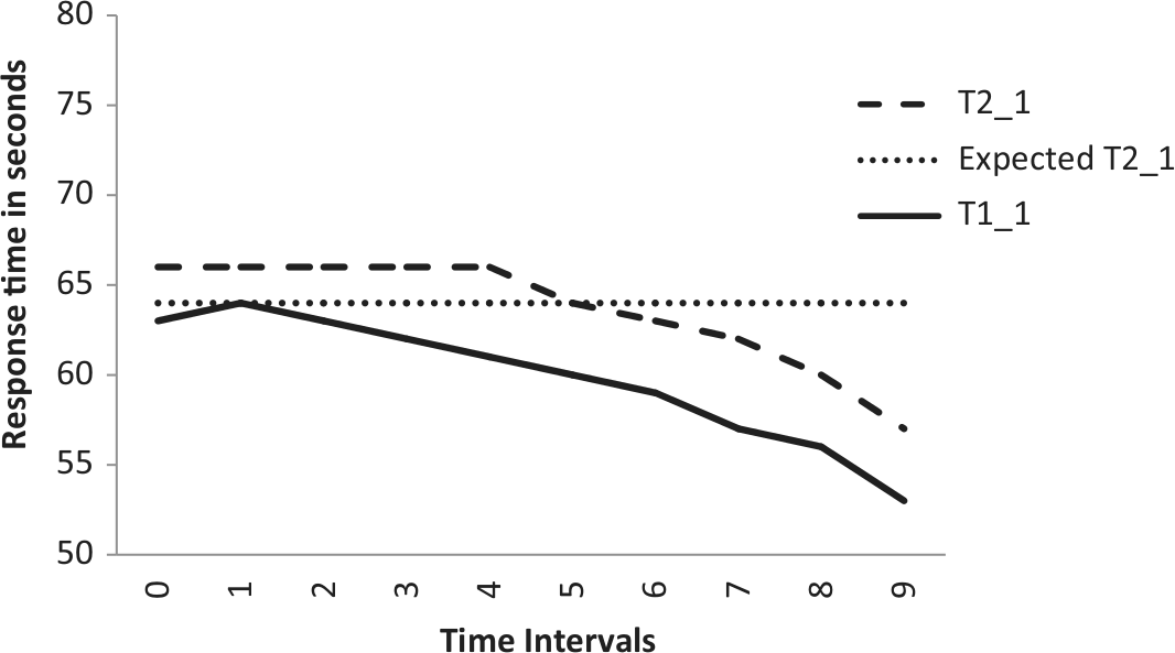
Expected and observed median response times for native language speakers for pre- (T1) and post-timing change (T2).

Growth curve modeling provides a comprehensive approach for modeling longitudinal item response time data. As illustrated, multigroup and piecewise models can be useful alternatives, for example, to single-group and quadratic models, providing comparable results and enhancing interpretation. The methodology is flexible in that both within- and between-examinee levels can be extended to include important predictor variables. There are several interesting areas of investigation for future work. One area might be extending the two-level model with no item effects to a three-level model with item effects. Another area may involve extending the model to estimate group membership as a time-invariant attribute at the individual level.