Coefficient Alpha and Reliability of Scale Scores

Abstract

The majority of large-scale assessments develop various score scales that are either linear or nonlinear transformations of raw scores for better interpretations and uses of assessment results. The current formula for coefficient alpha (α; the commonly used reliability coefficient) only provides internal consistency reliability estimates of raw scores. This article presents a general form of α and extends its use to estimate internal consistency reliability for nonlinear scale scores (used for relative decisions). The article also examines this estimator of reliability using different score scales with real data sets of both dichotomously scored and polytomously scored items. Different score scales show different estimates of reliability. The effects of transformation functions on reliability of different score scales are also explored.

Keywords

coefficient α internal consistency reliability scale scores classical test theory

Since its invention, coefficient alpha (α) has become the most commonly used coefficient for internal consistency reliability of test scores in theoretical and practical measurement research. This is partially due to its liberal assumptions, generalizability, and simplicity of computation. Coefficient α assumes that test forms (or even individual items) are essentially tau-equivalent, which implies that they measure the same construct on the same scale, but their means and standard deviations may vary (Graham, 2006). Coefficient α can be estimated from one administration of a single form of items or tasks scorable with any scoring pattern. It simply requires computing the sum of item score variances and raw score variances.

In spite of its generality, coefficient α provides only an estimate of reliability for raw scores or a linear transformation of them (e.g., average scores, linearly standardized scores, linearly equated scores, or any other linearly transformed scores). It is very rare that a large-scale assessment only reports raw scores on cognitive or noncognitive assessments. Raw scores are very difficult to interpret, as they lack a reference scheme to interpret examinees’ performances (Kolen & Lee, 2011). Raw scores are usually transformed nonlinearly to scale scores (Petersen, Kolen, & Hoover, 1989; Tong & Kolen, 2006). Kolen and Lee (2011) noted that due to interpretation and utilization issues along with the psychometric properties of test scores necessary to support an argument about test validity, one should consider both raw scores and scale scores or other indicators that are used for score reporting. There is a need to understand the extent to which score scales implemented by test developers ensure reliable and consistent interpretation and use of test results (Kolen & Lee, 2011).

However, the current uses of coefficient α do not facilitate estimating the reliability of scale scores resulting from nonlinear transformation of raw scores (Cronbach & Shavelson, 2004). This can be reasoned by the fact that scale scores are typically developed for the overall raw scores, not for individual items. However, coefficient α (in its current form) uses item scores to estimate the sum of item variances (an important term in coefficient α). Coefficient α reliability can facilitate estimating reliability for scale scores if the scale scores are obtained from transformed individual item scores, such as ones incorporating different item weights when computing raw scores (Feldt & Brennan, 1989). Still, nonlinear transformations of test scores are applied to the overall raw scores and not to individual items.

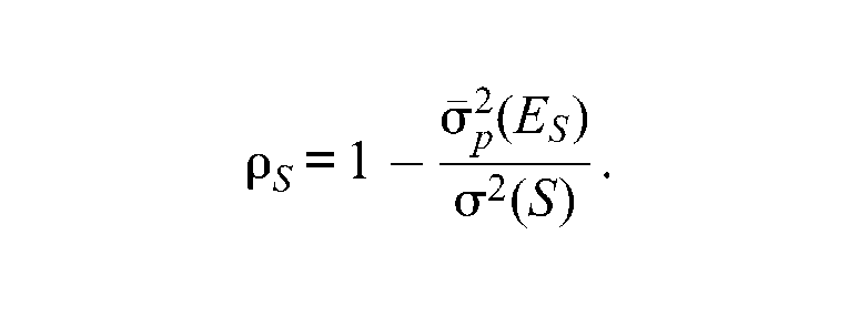
Alternative methods have been suggested for estimating the reliability of nonlinearly transformed scores within strong true-score theory, such as the binomial error model (Lord, 1965) or the multinomial error model. Other methods have been implemented using item response theory (IRT), such as dichotomous or polytomous IRT models. For these methods, the reader can refer to Brennan and Lee (1999); Feldt and Qualls (1998); Kolen, Hanson, and Brennan (1992); Kolen, Zeng, and Hanson (1996); Lee, Brennan, and Kolen (2000); and Lee (2007).

All these methods follow a similar scheme. First, they begin by choosing an appropriate strong error model for an individual person with a given test true/ability score. Strong error models can be a variety of other model types, such as a binomial model, a compound binomial model (Lee et al., 2000), a multinomial model, a compound multinomial model (Lee, 2007), a dichotomous IRT model (Kolen et al., 1996), or a polytomous IRT model (Wang, Kolen, & Harris, 2000). Second, the selected error model is then used to estimate the conditional scale error variance for each individual person, $σ_{p}^{2} (E_{S}),$ by using the raw-to-scale transformation, $s_{x}$ , used to build the score scale. Third, these conditional scale error variances are averaged over the whole sample of examinees to get the average scale error variance, ${\bar{σ}}_{p}^{2} (E_{S}) .$ Simultaneously, the observed scale score variance, $σ^{2} (S)$ , is calculated for the whole sample. Finally, these two variances are substituted into the classical definition of reliability to estimate the internal consistency reliability of scale scores; that is,

ρ_{S} = 1 - \frac{{\bar{σ}}_{p}^{2} (E_{S})}{σ^{2} (S)} .

Previous research (e.g., Feldt & Qualls, 1998; Kolen et al., 1992; Kolen & Lee, 2011; Lee, 2007; Lee et al., 2000) has studied the effects of nonlinear transformation functions on individual and average scale error variances and reliability. With binomial, multinomial, and IRT models, a transformation function with a large slope has been found to cause larger individual and average scale error variances, and vice versa. As a result, different score scales yield different reliability estimates than those from raw scores. Kolen and Lee (2011) and Lee (2007) further explained the effect of nonlinear transformation by the number of scale score points used for the score scale. Transforming raw scores to scale scores with a relatively larger number of score points results in a larger reliability estimate, and vice versa.

The previously discussed methods for estimating reliability for scale scores all require fitting a model for error scores. Model fit based on the assumptions required by these models needs to be checked with actual data before a full use. These assumptions are relatively stronger and more difficult to justify with real data in comparison with the assumptions required by classical test theory. For example, IRT models assume unidimensionality and local independence, and require an accurate estimation of item parameters and large sample sizes. The appropriateness of reliability estimates for scale scores by these methods is questionable if the assumed model does not fit the data.

In addition, the reliability estimates of test scores are different and not interchangeable under strong true-score theory and the classical test theory. They differ in how each theory defines equivalent test forms and the type of error score variance. While test forms in classical test theory (including coefficient α reliability) are classically (or rationally) parallel, they are also randomly parallel and equally difficult in strong true-score theory (Brennan & Lee, 1999; Feldt, 1984; Lee et al., 2000). Moreover, using generalizability theory terminology, coefficient α incorporates what is known as relative error score variance associated with relative decisions. However, the methods in strong true-score theory incorporate what is known as absolute error score variance associated with absolute decisions (Brennan, 2001).

The purpose of this article is to introduce a different form of coefficient α to facilitate its use in estimating reliability of scale scores (both linearly and nonlinearly transformed scale scores resulting from a norm-based process) under the assumption of classical test theory. Specifically, the goals of this article are (a) to outline a generalization of coefficient α reliability for scale scores for a set of items or tasks using any item scoring pattern, (b) to discuss the effects of transformation functions on the reliability of test scores, and (c) to explore the performance of the generalized coefficient α to estimate the reliability of different score scales for norm-referenced tests (specifically, raw scores, unrounded (USS) and rounded (RSS) linear standard scores, unrounded (UNSS) and rounded (RNSS) normalized standard scores, percentile ranks [PR], and stanines). Different real data sets are analyzed, including a cognitive assessment with dichotomously scored items and a noncognitive assessment with polytomously scored items.

Coefficient α

This section presents different forms of coefficient α reliability with different interpretations of its components. Following that, a generalized form of coefficient α reliability is outlined for estimating reliability of scale scores.

Different Forms of Coefficient α

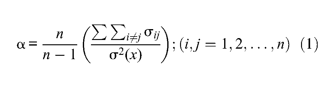
Coefficient α is commonly used to estimate the reliability of raw scores composed of $n$ items that are either dichotomously or polytomously scored. Under the assumption of essentially tau-equivalent test forms, a common form of coefficient α is

α = \frac{n}{n - 1} (\frac{\sum^{​} \sum_{i \neq j} σ_{i j}}{σ^{2} (x)}); (i, j = 1, 2, \dots, n)

where $\sum \sum_{i \neq j} σ_{ij}$ is the accumulated sum of inter-item covariances and $σ^{2} (x)$ is the observed raw score variance. Cronbach (1951) stated that “this important relation states a clear meaning for α as $n / (n - 1)$ times the ratio of inter-item covariance to total variance” (p. 305).

The accumulated sum of inter-item covariances is typically difficult to obtain, especially with a large number of items. However, another commonly cited form for coefficient α recognizes the linear decomposition of variance of raw scores that are a linear unweighted composite of item scores; that is,

σ^{2} (x) = \sum_{i} σ_{i}^{2} + \sum^{​} \sum_{i \neq j} σ_{i j}; (i, j = 1, 2, \dots, n),

where $\sum_{i} σ_{i}^{2}$ is the sum of individual item variances. The individual item variances are computed using the observed item scores for all sampled individuals. Solving for $\sum \sum_{i \neq j} σ_{ij}$ in Equation 2, coefficient α becomes

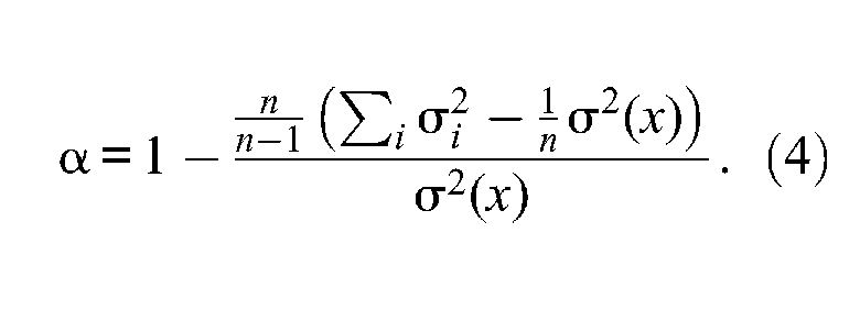
α = \frac{n}{n - 1} (\frac{σ^{2} (x) - \sum_{i} σ_{i}^{2}}{σ^{2} (x)}) = \frac{n}{n - 1} (1 - \frac{\sum_{i} σ_{i}^{2}}{σ^{2} (x)}) .

Now, with a simple manipulation of Equation 3, coefficient α can be rewritten in a very useful form as follows:

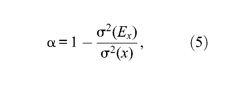
α = 1 - \frac{\frac{n}{n - 1} (\sum_{i} σ_{i}^{2} - \frac{1}{n} σ^{2} (x))}{σ^{2} (x)} .

Equation 4 suggests that coefficient α can be defined as the classical definition of reliability (under the assumption of uncorrelated error scores) with a specific estimator of error score variance; that is,

α = 1 - \frac{σ^{2} (E_{x})}{σ^{2} (x)},

where

σ^{2} (E_{x}) = \frac{n}{n - 1} (\sum_{i} σ_{i}^{2} - \frac{1}{n} σ^{2} (x)) .

The first term in Equation 6, $\sum_{i} σ_{i}^{2},$ is the sum of item variances, which represents the variance of raw scores if there were no communalities among items ( $\sum \sum_{i \neq j} i \neq j$ ). The second term in Equation 6, $σ^{2} (x),$ is the observed variance of raw scores that depicts any communality existing among test items. $σ^{2} (x)$ can have values that are either larger or smaller than $\sum_{i} σ_{i}^{2}$ depending on the inter-item correlations. It is larger than $\sum_{i} σ_{i}^{2}$ when test items are positively intercorrelated and smaller than $\sum_{i} σ_{i}^{2}$ when test items are negatively intercorrelated. Definitely, for raw scores to be highly reliable, test items should be positively intercorrelated, and consequently, $σ^{2} (x)$ should be much larger than $\sum_{i} σ_{i}^{2} .$

The classical definition of reliability necessitates that coefficient α yield reliability estimates in the range of 0 and 1. This implies that valid values of $σ^{2} (E_{x})$ should be bounded by $0 \leq σ^{2} (E_{x}) \leq σ^{2} (x)$ . However, since coefficient α is merely an estimator of test score reliability with sampled data, it is possible that the estimated values of coefficient α and its associated error score variance, $σ^{2} (E_{x}),$ can be outside of their acceptable ranges. In cases where $σ^{2} (E_{x})$ is less than zero, it should be intuitively set to zero; then α will be equal to one, indicating a perfect reliability. When $σ^{2} (E_{x})$ exceeds $σ^{2} (x),$ it implies that test items are negatively intercorrelated. A relatively larger $σ^{2} (E_{x})$ than $σ^{2} (x)$ threatens test score reliability and results in a negative α. In such cases, α is typically set to zero, indicating there is no test score reliability (Cronbach, 1951).

Returning to the first term in Equation 6, $\sum_{i} σ_{i}^{2},$ the sum of item variances represents the raw score variance estimated from the sampled data if examinees are believed to respond independently to test items and there is no communality among test items (uncorrelated error scores). This means that $\sum_{i} σ_{i}^{2}$ is the variance of the distribution of raw scores conditioned on the observed proportions of item score points under the assumption of both independent item responses and uncorrelated error scores. In fact, Kuder and Richardson (1937) similarly interpreted the term $\bar{p} \bar{q}$ in KR-21 (KR-21 is a special case of coefficient α, when dichotomously scored items are equally difficult). “ $n \bar{p} \bar{q}$ is the variance of n equally difficult items when they are uncorrelated, by the familiar binomial theory” (Kuder & Richardson, 1937, p. 159).

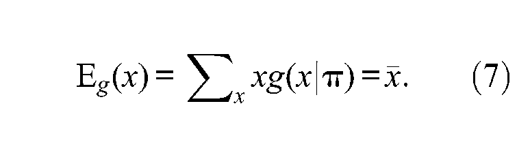
Symbolically, suppose that the distribution of raw scores conditioned on the observed proportions of item score points (e.g., for dichotomous items, the proportion getting the item right and the proportion getting the item wrong) for all items on the test under the assumption of independent item responses and uncorrelated error scores is known, and say $g (x | π),$ where $π$ is the $n \times K$ matrix of the proportions of item score points (where $n$ is number of items and $K$ is number of score points per item). Using the observed proportions of item score points from the sampled data, $π$ , the average score for this conditional distribution function is equal to the observed average test score, $\bar{x}$ , and is referred to as

E_{g} (x) = \sum_{x} xg (x | π) = \bar{x} .

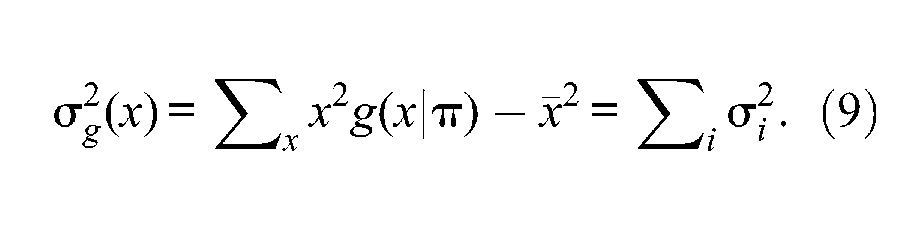
The variance of this conditional distribution function is defined as (referred here as $σ_{g}^{2} (x)$ ),

σ_{g}^{2} (x) = \sum_{x} {[x - E_{g} (x)]}^{2} g (x | π) = \sum_{x} x^{2} g (x | π) - {\bar{x}}^{2},

which gives the required sum of item variances estimated from the sampled data, $\sum_{i} σ_{i}^{2}$ ; that is,

σ_{g}^{2} (x) = \sum_{x} x^{2} g (x | π) - {\bar{x}}^{2} = \sum_{i} σ_{i}^{2} .

Now, by substituting this new estimator of $\sum_{i} σ_{i}^{2}$ into Equations 5 and 6, coefficient α becomes

α = 1 - \frac{σ^{2} (E_{x})}{σ^{2} (x)},

where

σ^{2} (E_{x}) = \frac{n}{n - 1} (σ_{g}^{2} (x) - \frac{1}{n} σ^{2} (x)), 0 \leq σ^{2} (E_{x}) \leq σ^{2} (x) .

Hence, coefficient α reliability of raw scores can be equivalently computed using Equation 1, 3, 5, or 10. This is a mathematical identity, not an approximation.

The new form of coefficient α (Equation 10) has an advantage over its typical form since it does not require computing item score variance at individual item level. Rather, it uses the variance for the conditional distribution of raw scores. This advantage allows extending coefficient α to estimate the reliability of scale scores that result from direct transformation of raw scores.

Coefficient Generalized α Reliability for Scale Scores, Gα_s

Score scales are often formed by transforming raw scores so that the resulting scale scores have certain desirable properties and interpretations. Interpretations of test scores can be facilitated by incorporating either normative meaning (through a norming-based mechanism) or content and criterion meaning (through a criterion-based mechanism; Kolen & Lee, 2011). The process of incorporating normative meaning into score scales requires collecting test score data on a relevant, recent, and representative norm group. Examples of normative-based score scales are PR, standard scores, normalized standard scores, and grade equivalents. The process of incorporating content and criterion meaning into scale scores requires defining scale scores for tests measuring well-defined item domains with reference to specific levels of achievement or identified judgmental standards of quality (Petersen et al., 1989). Examples of criterion-based score scales are percentage correct scores, standard levels on performance assessment, and achievement levels.

The raw-to-scale transformation function can be linear or nonlinear. A linear transformation function involves establishing a new location and spread of raw scores without altering their distributional shape. A nonlinear transformation function can take any monotonically nondecreasing form, which typically results in altering the distributional shape of the original raw scores. With nonlinear transformations, raw scores can be transformed into almost any prespecified distributional shape for a particular group of examinees. A simple example of nonlinear transformation is the truncation of a linear transformation of raw scores at any arbitrarily selected raw score value. For example, scale scores can be obtained through a linear transformation and then by setting the maximum scale score equal to 95% of the maximum possible raw score value, and setting the chance raw score value as the minimum scale score. Raw scores above the 95% of maximum raw scores will be truncated to the maximum scale score, and raw scores below the chance raw score will be truncated to the minimum scale score.

Coefficient α can be used to estimate reliability of scale scores built using normative-based scaling. With normative-based scale scores, the investigator’s interest focuses on the relative ordering of examinees with respect to the performance for the norm group that the examinee is associated with (Brennan, 2001). In such cases, error score variance is defined as the expected squared difference between an examinee’s observed deviation score (from the examinee’s true score) and the associated group’s observed deviation score. This error score variance is incorporated in coefficient α (Cronbach, Gleser, Nanda, & Rajaratnam, 1972).

However, it is not advisable to use coefficient α to estimate reliability of scale scores that are built using criterion-based scaling. In such cases, the investigator’s interest focuses typically on absolute interpretations of scores and absolute error score variance (Brennan, 2001). Absolute error score variance is defined as the expected squared difference between an examinee’s observed score and his or her true score. To estimate the reliability of such scale scores, other existing methods should be used, such as those suggested by Brennan and Lee (1999), Feldt and Qualls (1998), Kolen et al. (1992, 1996), Lee et al. (2000), Lee (2007), and Kolen, Wang, and Lee (2012).

In this article, a scale score is defined as any scale score metric that results from any raw-to-scale transformation function of a raw score metric that incorporates a relative interpretation of the scores. Now, suppose that a discrete raw-to-scale transformation function exists, symbolized as $s_{x}$ , and suppose that it is used to transform raw scores into scale scores through a normative process (for each $x$ , there is a unique $s_{x}$ ). The function $s_{x}$ can be either one-to-one (every distinct $x$ is converted to a unique value of $s_{x}$ ) or many-to-one (several $x$ values are converted to a unique value of $s_{x}$ ).

Using the discrete raw-to-scale transformation, the average and variance of scale scores, assuming independent item responses and uncorrelated error scores, can be obtained using the conditional distribution $g (x | π)$ , respectively, through

E_{g} (s) = \sum_{x} s_{x} g (x | π) and σ_{g}^{2} (s) = \sum_{x} s_{x}^{2} g (x | π) - {[E_{g} (s)]}^{2} .

However, the observed average and observed variance of scale scores can be obtained from the sample after converting raw scores to their corresponding scale scores for all individuals. Similarly, using the observed relative frequency of raw scores obtained from the sample, say $f (x)$ , both observed average and observed variance of scale scores can be obtained, respectively, through

E (s) = \sum_{x} s_{x} f (x) and σ^{2} (s) = \sum_{x} s_{x}^{2} f (x) - {[E (s)]}^{2} .

Note that these last two forms are very useful when the test’s investigator is concerned about the reliability coefficients for different score scales without converting all individuals’ raw scores to their corresponding scale scores.

Now, the reliability of scale scores can be easily obtained with coefficient α by substituting $σ_{g}^{2} (s)$ (Equation 12) and $σ^{2} (s)$ (Equation 13) into Equation 10. To differentiate coefficient α reliability for scale scores from coefficient α reliability for raw scores, the new coefficient will be called coefficient generalized alpha reliability. It will be referred to as $G α_{S} .$ $G α_{S}$ will designate the reliability estimator of any score scale, whereas α will designate the reliability estimator of raw scores:

G α_{s} = 1 - \frac{σ^{2} (E_{s})}{σ^{2} (s)}

where

σ^{2} (E_{s}) = \frac{n}{n - 1} (σ_{g}^{2} (s) - \frac{1}{n} σ^{2} (s)), 0 \leq σ^{2} (E_{s}) \leq σ^{2} (s) .

$σ^{2} (E_{s})$ is the overall scale error variance and should be in the range of $0 \leq σ^{2} (E_{s}) \leq σ^{2} (s) .$ If it happens that the value of $σ^{2} (E_{s})$ is less than zero as a result of raw-to-scale transformation functions, it should be set to zero; then $G α_{S}$ will be equal to one, indicating a perfect reliability. Similarly, if the value of $σ^{2} (E_{s})$ is larger than $σ^{2} (s)$ , $G α_{S}$ should be set to zero, indicating absence of reliability.

Following the pattern of all the published derivations of coefficient α and related coefficients (e.g., Cronbach, 1951; Guttman, 1945; Hoyt, 1941; Kuder & Richardson, 1937), making the same assumptions but imposing no limit on both the scoring of test items and the scaling of raw scores (for relative interpretation) will permit the derivation of Equation 14.

Equation 10 for coefficient α reliability of raw scores and Equation 14 for coefficient $G α_{S}$ reliability of scale scores require computing only two variances. These are $σ_{g}^{2} (s)$ , the raw/scale score variance assuming independent item responses and uncorrelated error scores, and $σ^{2} (s)$ , the observed raw/scale score variance.

General Method to Obtain g(x|π)

$g (x | π)$ represents the distribution of raw scores conditioned on the matrix of the observed proportions of item score points under the assumption of independent item responses and uncorrelated error scores. Unfortunately, it is not straightforward and easy to obtain $g (x | π) .$ It differs for different methods of scoring test items. For example, when items are dichotomously scored, $g (x | π)$ can be considered as a compound binomial with $n$ and different proportions correct for each item, $p_{i}$ . When items are polytomously scored, $g (x | π)$ is a compound multinomial distribution with $n$ and different proportions of various possible scores, $c_{k}$ ( $k = 1, 2, \dots, K$ ), on each item, $p_{i} (c_{k})$ .

A single recursive formula is introduced here to compute $g (x | π)$ for various item scoring methods. The formula is adopted from Hanson (1994) and Thissen, Pommerich, Billeaud, and Williams (1995), and it is a generalized form of the Lord and Wingersky (1984) recursion formula. This formula is commonly used in the context of IRT. Generally, this recursion formula gives a probability mass function of raw scores on a test of $n$ items using probabilities (or proportions) of possible item scores under the assumption of independent item responses. In an IRT context, the probabilities of possible item scores are obtained from the adopted-IRT model for a given ability value. Here, the probabilities of possible item scores are replaced by as the observed proportions of possible item scores for each individual item on the test.

To use the recursion formula to obtain $g (x | π)$ , suppose there is a test of $n$ items or tasks ( $i = 1, 2, \dots, n$ ) with any number of possible item score points with an increment of d, $c_{k}$ ( $k = 1, 2, \dots, K$ ) administered to a sample of size $N (j = 1, 2, \dots, N) .$ The items have a similar number of possible scores, K. Although it is not a necessary requirement, the increment, d, is typically one. $u_{i}$ represents an observed score of a person on a single item, i, which could be one and only one of many possible scores, $c_{k} .$ $x = \sum_{i} u_{i}$ is the raw score, which is the sum of examinees’ item scores. It ranges between $n c_{1}$ to $n c_{K}$ with an increment of d. From the sample data, the observed proportions of each item score point, $p_{i} (c_{k})$ , can be obtained. These points, $p_{i} (c_{k}),$ represent the proportions of examinees who respond to or obtain each score point, $c_{k},$ on each item, i.

To get $g (x | π)$ through the recursion formula, define $X_{i}$ as the random variable of raw scores on the first i items on the test ( $X_{i}$ ranges between $i c_{1}$ and $i c_{K}$ ). Now, let $g (X_{i} = x_{i} | π_{i})$ represent the probability mass function of $X_{i}$ when it is equal to $x_{i}$ on a test of $i$ items. For a test of one item, $i = 1$ is entered into the formula

g (X_{1} = x_{1} = c_{k} | π_{1}) = p_{1} (c_{k}), for x_{1} = c_{1}, c_{2}, \dots, c_{K} .

For the next $i > 1,$ the recursion formula is as follows:

g (X_{i} = x_{i} | π_{i}) = \sum_{k = 1}^{K} g (X_{i - 1} = x_{i} - c_{k} | π_{i - 1}) p_{i} (c_{k}), for x_{i} = i c_{1}, i c_{1} + d, \dots, i c_{K} .

To use this recursion formula, enter items into the recursion formula in any order, beginning with $i = 1,$ and repeatedly apply the formula by increasing $i$ on each repetition. The process is stopped after $i = n$ , which gives the required $g (x | π) .$ That is, $g (x | π) = g (X_{n} = x_{n} = x | π) .$

Effect of Transformation Function on Reliability of Test Scores

As a result of nonlinear transformation functions, the shape of both the observed distribution and conditional distribution of scale scores will be altered in comparison with $f (x)$ and $g (x | π)$ for the corresponding raw scores. In addition, the extent of this alteration in the distributional shapes will not be necessarily similar for both $g (x | π)$ and $f (x) .$ Moreover, the extent of this alternation might differ from one raw-to-scale transformation function to another. As a result, the magnitude of the effect of any specific raw-to-scale transformation function on $σ_{g}^{2} (s)$ , $σ^{2} (s)$ , $σ^{2} (E_{s})$ , and $G α_{S}$ reliabilities of test scores cannot be predetermined since all these quantities are functions of $g (x | π)$ and/or $f (x)$ . However, the direction of the effect of any specific raw-to-scale transformation function on the reliability of test scores might be projected. The following demonstration can help in perceiving the direction of the effect of any transformation function on coefficient $G α_{S}$ relative to α.

Consider two ratios quantifying the average effect on $σ_{g}^{2} (s)$ and $σ^{2} (s)$ relative to their counterparts $σ_{g}^{2} (x)$ and $σ^{2} (x)$ as a result of a certain raw-to-scale transformation function used to build the scale scores. Although the effect of the transformation function differs from one scale score to another, these two ratios summarize the average effects of this transformation function on these two variances along the score scale; that is,

a_{1} = \frac{σ^{2} (s)}{σ^{2} (x)}, and a_{2} = \frac{σ_{g}^{2} (s)}{σ_{g}^{2} (x)} .

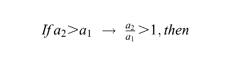
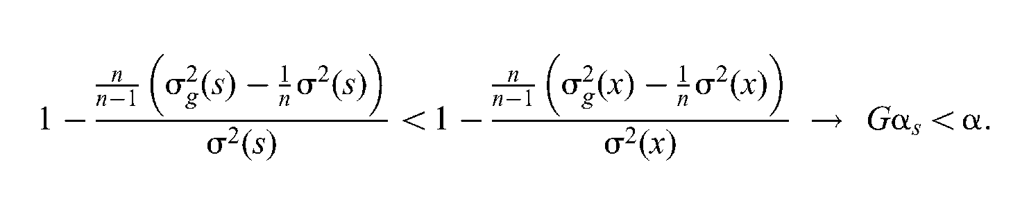
Considering the three possibilities of inequality of $a_{2}$ and $a_{1}$ ( $>$ , $=$ , $<$ ), how does $G α_{S}$ differ from α? For simplicity, one inequality ( $<$ ) of $a_{2}$ and $a_{1}$ is demonstrated:

If a_{2} > a_{1} \to \frac{a_{2}}{a_{1}} > 1, then

\to \frac{a_{2}}{a_{1}} \frac{σ_{g}^{2} (x)}{σ^{2} (x)} - \frac{1}{n} > \frac{σ_{g}^{2} (x)}{σ^{2} (x)} - \frac{1}{n} \to \frac{a_{2} σ_{g}^{2} (x) - \frac{1}{n} a_{1} σ^{2} (x)}{a_{1} σ^{2} (x)} > \frac{σ_{g}^{2} (x) - \frac{1}{n} σ^{2} (x)}{σ^{2} (x)} 1 - \frac{\frac{n}{n - 1} (a_{2} σ_{g}^{2} (x) - \frac{1}{n} a_{1} σ^{2} (x))}{a_{1} σ^{2} (x)} < 1 - \frac{\frac{n}{n - 1} (σ_{g}^{2} (x) - \frac{1}{n} σ^{2} (x))}{σ^{2} (x)} .

Now from Equations 10, 14, and 18,

1 - \frac{\frac{n}{n - 1} (σ_{g}^{2} (s) - \frac{1}{n} σ^{2} (s))}{σ^{2} (s)} < 1 - \frac{\frac{n}{n - 1} (σ_{g}^{2} (x) - \frac{1}{n} σ^{2} (x))}{σ^{2} (x)} \to G α_{s} < α .

Similar demonstrations can be replicated with the other two possibilities of inequalities ( $=$ , $<$ ) of $a_{2}$ and $a_{1}$ . The effects of a transformation function on $G α_{S}$ are summarized as follows:

G α_{s} = α if a_{2} = a_{1},

The first effect is observed with linearly transformed scale scores. The two ratios are equal with any linear transformation function and equal to the slope of this transformation function. The linear transformation function similarly affects the two test score variances, resulting in invariant reliability of the linearly transformed scale scores and the original raw scores.

The other two effects are observed with nonlinear transformation functions. For a nonlinear transformation function, the slope is different across the raw score metric and the distribution of $f (x)$ and $g (x | π)$ . These two ratios are not necessarily equal for the same transformation function, thus resulting in different effects on the two test score variances. This depends on the distribution of raw scores, $f (x)$ and $g (x | π)$ , associated with these two variances. As a result, the reliability coefficient of nonlinearly transformed scale scores differs from the reliability coefficient of the original raw scores (either larger or smaller). The reliability of scale scores will be smaller than the reliability of raw scores if $a_{2} > a_{1}$ . However, the reliability of scale scores will be larger than the reliability of raw scores if $a_{2} < a_{1}$ . The degree of effect from a transformation function on the reliability coefficient of scale scores does not depend on the numerical magnitude of either $a_{1}$ or $a_{2}$ (large or small average slope) but rather on their ratio. Whenever this ratio goes farther from unity, the degree of the effect from a transformation function on the reliability of test scores (either increasing or decreasing) becomes larger (more or less), and vice versa.

Let us consider, for example, percentile ranks (PR) scores as one commonly used score scale. PR scores for raw scores with $f (x)$ of a normal distribution would show a reliability estimate that is less than the reliability estimate of the original raw scores. This could be explained by the following argument: Raw scores of a normal distribution show a larger number of raw scores in the middle of the score metric relative to the two tails of the score metric. As a result, those raw scores in the middle of the score metric (with larger number of examinees) are transformed to more deviated PR scores, and those raw scores in the two tails of the score metric are transformed to less deviated PR scores. This should cause a relatively larger $σ^{2} (s)$ for PR scores than $σ^{2} (x)$ for raw scores. Similarly, if we assume that $g (x | π)$ for the same raw scores is also normally distributed (could be obtained when item averages are not extreme), then this $g (x | π)$ should have a more peaked distribution at the middle of the score metric when compared with $f (x)$ . PR scores should then show a larger $σ_{g}^{2} (s)$ than $σ_{g}^{2} (x)$ and a larger than $σ^{2} (s)$ , by which the $G α_{S}$ reliability estimate for PR scores should be smaller than for raw scores.

However, if UNSS are used as scale scores with similar test specifications as before, their reliabilities will be larger than the reliability of raw scores. Raw scores in the middle of the score metric are transformed to less deviated UNSS scores, whereas raw scores in the two tails of the score metric are transformed to more deviated UNSS scores. Since $g (x | π)$ is more peaked than is $f (x)$ at the middle of the score metric, $σ_{g}^{2} (s)$ for UNSS scores will be smaller than $σ^{2} (s)$ , by which the $G α_{S}$ reliability estimate for UNSS scores will be larger than that for raw scores.

Different distribution shapes of $g (x | π)$ with different score scales should make $σ_{g}^{2} (s)$ unchanged, larger, or smaller than $σ_{g}^{2} (x)$ . This might result in reliability estimates of scale scores that are similar, smaller, or larger than the reliability of the original raw scores, respectively. These relationships depend heavily on the distributional shape of both $f (x)$ and $g (x | π),$ and the raw-to-scale transformation function used.

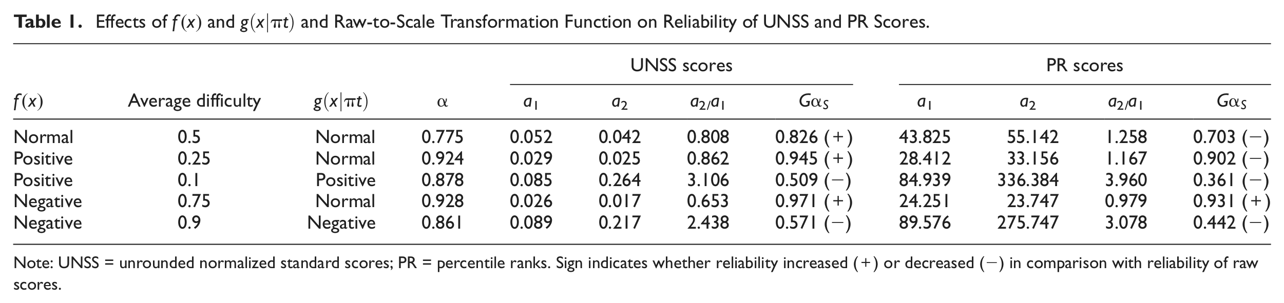
To further explain the relationship between the distributional shape of both $f (x)$ and $g (x | π),$ and $G α_{S}$ for different score scales, Table 1 presents the results of simulated data examining the effects of $f (x)$ and $g (x | π)$ on $G α_{S}$ reliability of PR and UNSS scores (M of 0 and SD of 1). With a test of 20 dichotomously scored items, responses for 5,000 individuals were randomly generated using a two-parameter IRT model for different distributional shapes of $f (x)$ (normal, negatively skewed, positively skewed) and different average item difficulty (easy, medium, difficult). Different average item difficulties were chosen to create different distributional shapes of $g (x | π)$ . Results showed that $G α_{S}$ for PR scores were smaller than reliability estimates for raw scores for all simulated distributions, except when $f (x)$ was negatively skewed and $g (x | π)$ was normally distributed). However, $G α_{S}$ for UNSS scores were larger than reliability estimates for raw scores when $g (x | π)$ was normally distributed). $G α_{S}$ for UNSS scores were smaller than reliability estimates for raw scores when $g (x | π)$ was positively and negatively skewed, respectively). These results also support the established relationship between the ratios of $a_{1}$ and $a_{2},$ and the reliability of scale scores (Equations 17 and 18).

Table 1.

Effects of $f (x)$ and $g (x | π t)$ and Raw-to-Scale Transformation Function on Reliability of UNSS and PR Scores.

				UNSS scores				PR scores
$f (x)$	Average difficulty	$g (x \| π t)$	α	a ₁	a ₂	a ₂ _/a ₁	$G α_{S}$	a ₁	a ₂	a ₂ _/a ₁	$G α_{S}$
Normal	0.5	Normal	0.775	0.052	0.042	0.808	0.826 (+)	43.825	55.142	1.258	0.703 (−)
Positive	0.25	Normal	0.924	0.029	0.025	0.862	0.945 (+)	28.412	33.156	1.167	0.902 (−)
Positive	0.1	Positive	0.878	0.085	0.264	3.106	0.509 (−)	84.939	336.384	3.960	0.361 (−)
Negative	0.75	Normal	0.928	0.026	0.017	0.653	0.971 (+)	24.251	23.747	0.979	0.931 (+)
Negative	0.9	Negative	0.861	0.089	0.217	2.438	0.571 (−)	89.576	275.747	3.078	0.442 (−)

Note: UNSS = unrounded normalized standard scores; PR = percentile ranks. Sign indicates whether reliability increased (+) or decreased (−) in comparison with reliability of raw scores.

Comparing α and Gα_s With Dichotomously Scored Items

The procedure for estimating $G α_{S}$ reliability for scale scores is useful in a variety of practical situations. In this section, the procedure is applied to dichotomously scored items on a cognitive assessment and compared with α for raw scores. The assessment consists of three ability subtests on the Gulf Multiple Mental Abilities Scale.

Sample and Instrument

A sample of 1,886 students (males and females) were selected from all second graders who took the Gulf Multiple Mental Abilities Scale in 2010 as a part of the scaling process of the test. The test consists of three subtests: Verbal ability, Quantitative ability, and Spatial ability. The three subtests aim to measure different abilities of children from Grade 1 through Grade 6. Each ability subtest consists of 30 multiple-choice items. Each ability subtest is scaled separately using a developmental scale as a primary score scale. In addition, there are three auxiliary score scales for each ability subtest within each grade: UNSS with a mean of 100 and a standard deviation of 10, PR ranging between 1 and 99, and stanine scores ranging between 1 and 9 with a mean of 5. UNSS, PR, and stanines are monotonically increasing nonlinear transformations of raw scores.

Procedure

For the sake of comparisons, six score scales were computed for the three subtests of the Gulf Multiple Mental Abilities Scale: USS, RSS, UNSS, RNSS, PR, and stanines. USS is a linear transformation of raw scores to scale scores with a mean of 50 and a standard deviation of 10. RSS scores are USS scores rounded to the nearest integer. The other score scales are described earlier. Similarly, RNSS scores are UNSS scores rounded to the nearest integer. Both coefficient α and coefficient $G α_{S}$ reliability for the Gulf Multiple Mental Abilities Scale were computed for raw scores and these six score scales.

The proportions of correct and incorrect responses to each of the 30 items within each subtest were computed and used in the computation of α and $G α_{S} .$ Table 2 presents the descriptive statistics for these proportions and item averages. Table 2 shows that the items had variable item averages (item difficulty). Quantitative items showed the most variable item averages ( $σ_{d} = 0.212$ ) and the Verbal subtest had the least variable item averages ( $σ_{d} = 0.125$ ). Spatial items had relatively moderate variable item averages ( $σ_{d} = 0.158$ ).

Table 2.

Descriptive Statistics of Proportions of Item Scores and Item Averages for Items in the Three Subtests: Verbal, Quantitative, and Spatial.

	Verbal subtest			Quantitative subtest			Spatial subtest
	$p_{i} (c_{1} = 0)$	$p_{i} (c_{2} = 1)$	Items	$p_{i} (c_{1} = 0)$	$p_{i} (c_{2} = 1)$	Items	$p_{i} (c_{1} = 0)$	$p_{i} (c_{2} = 1)$	Items
Minimum	0.091	0.438	0.438	0.041	0.270	0.270	0.223	0.201	0.270
Maximum	0.562	0.909	0.909	0.730	0.959	0.959	0.799	0.777	0.959
M	0.354	0.646	0.646	0.443	0.557	0.557	0.569	0.431	0.557
SD	0.125	0.125	0.125	0.212	0.212	0.212	0.158	0.158	0.158

Results and Discussion

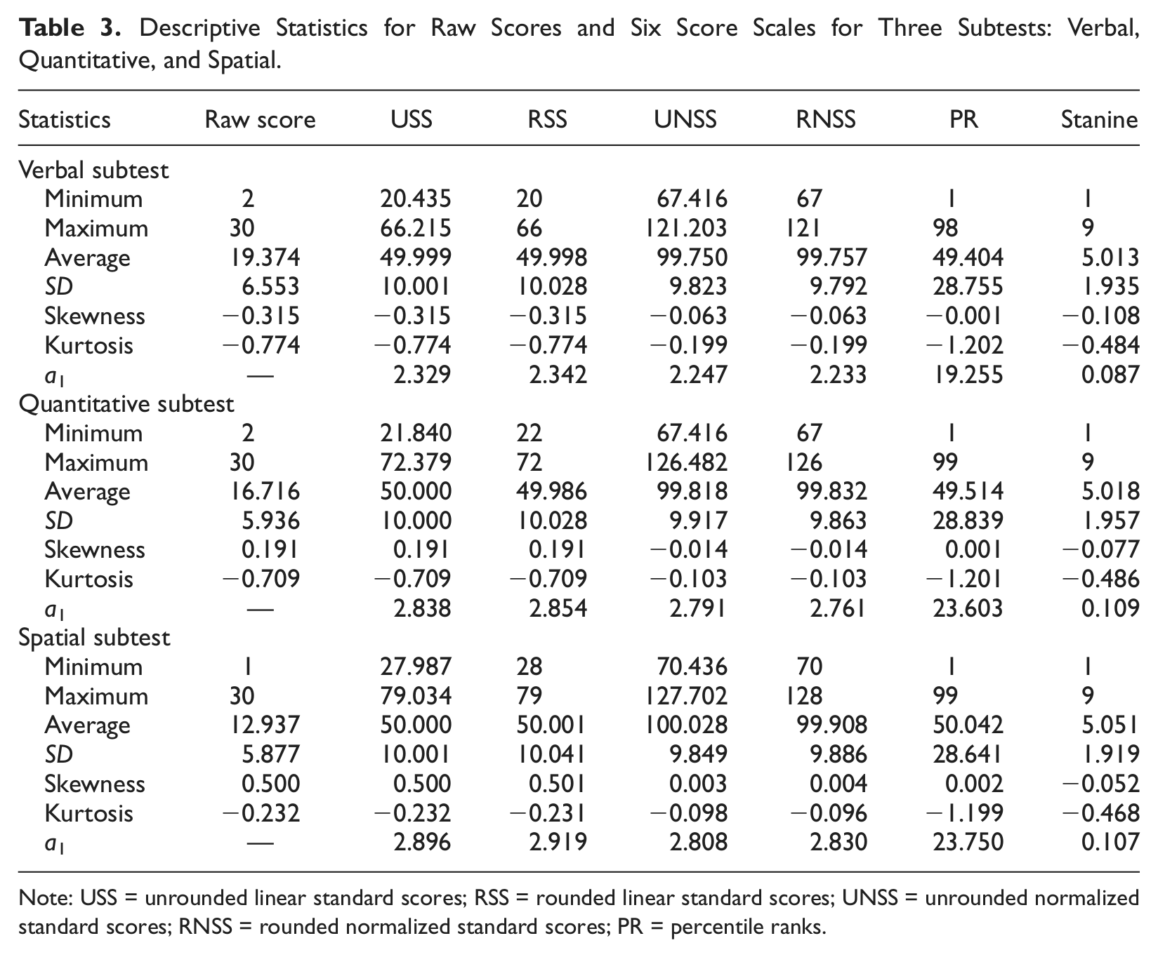
Table 3 presents the descriptive statistics for raw scores and the six score scales for the three subtests. The average raw score was 19.374 for the Verbal subtest, 16.716 for the Quantitative subtest, and 12.937 for the Spatial subtest. In addition, raw scores for the three subtests differed in their standard deviations, skewness, and kurtosis. As displayed in Table 3, each of the score scales had different scale values for the three subtests, and consequently different means, standard deviations, skewness, and kurtosis. Table 3 also presents the effect of a transformation function, $a_{1}$ , on the observed test score variance for each score scale. Except for the stanine scores, all the $a_{1}$ effects for different score scales were greater than one, which enlarged the observed scale score variances for the three subtests. The largest effect was observed in PR scores because of their wide scale range.

Table 3.

Descriptive Statistics for Raw Scores and Six Score Scales for Three Subtests: Verbal, Quantitative, and Spatial.

Statistics	Raw score	USS	RSS	UNSS	RNSS	PR	Stanine
Verbal subtest
Minimum	2	20.435	20	67.416	67	1	1
Maximum	30	66.215	66	121.203	121	98	9
Average	19.374	49.999	49.998	99.750	99.757	49.404	5.013
SD	6.553	10.001	10.028	9.823	9.792	28.755	1.935
Skewness	−0.315	−0.315	−0.315	−0.063	−0.063	−0.001	−0.108
Kurtosis	−0.774	−0.774	−0.774	−0.199	−0.199	−1.202	−0.484
a₁	—	2.329	2.342	2.247	2.233	19.255	0.087
Quantitative subtest
Minimum	2	21.840	22	67.416	67	1	1
Maximum	30	72.379	72	126.482	126	99	9
Average	16.716	50.000	49.986	99.818	99.832	49.514	5.018
SD	5.936	10.000	10.028	9.917	9.863	28.839	1.957
Skewness	0.191	0.191	0.191	−0.014	−0.014	0.001	−0.077
Kurtosis	−0.709	−0.709	−0.709	−0.103	−0.103	−1.201	−0.486
a₁	—	2.838	2.854	2.791	2.761	23.603	0.109
Spatial subtest
Minimum	1	27.987	28	70.436	70	1	1
Maximum	30	79.034	79	127.702	128	99	9
Average	12.937	50.000	50.001	100.028	99.908	50.042	5.051
SD	5.877	10.001	10.041	9.849	9.886	28.641	1.919
Skewness	0.500	0.500	0.501	0.003	0.004	0.002	−0.052
Kurtosis	−0.232	−0.232	−0.231	−0.098	−0.096	−1.199	−0.468
a₁	—	2.896	2.919	2.808	2.830	23.750	0.107

Note: USS = unrounded linear standard scores; RSS = rounded linear standard scores; UNSS = unrounded normalized standard scores; RNSS = rounded normalized standard scores; PR = percentile ranks.

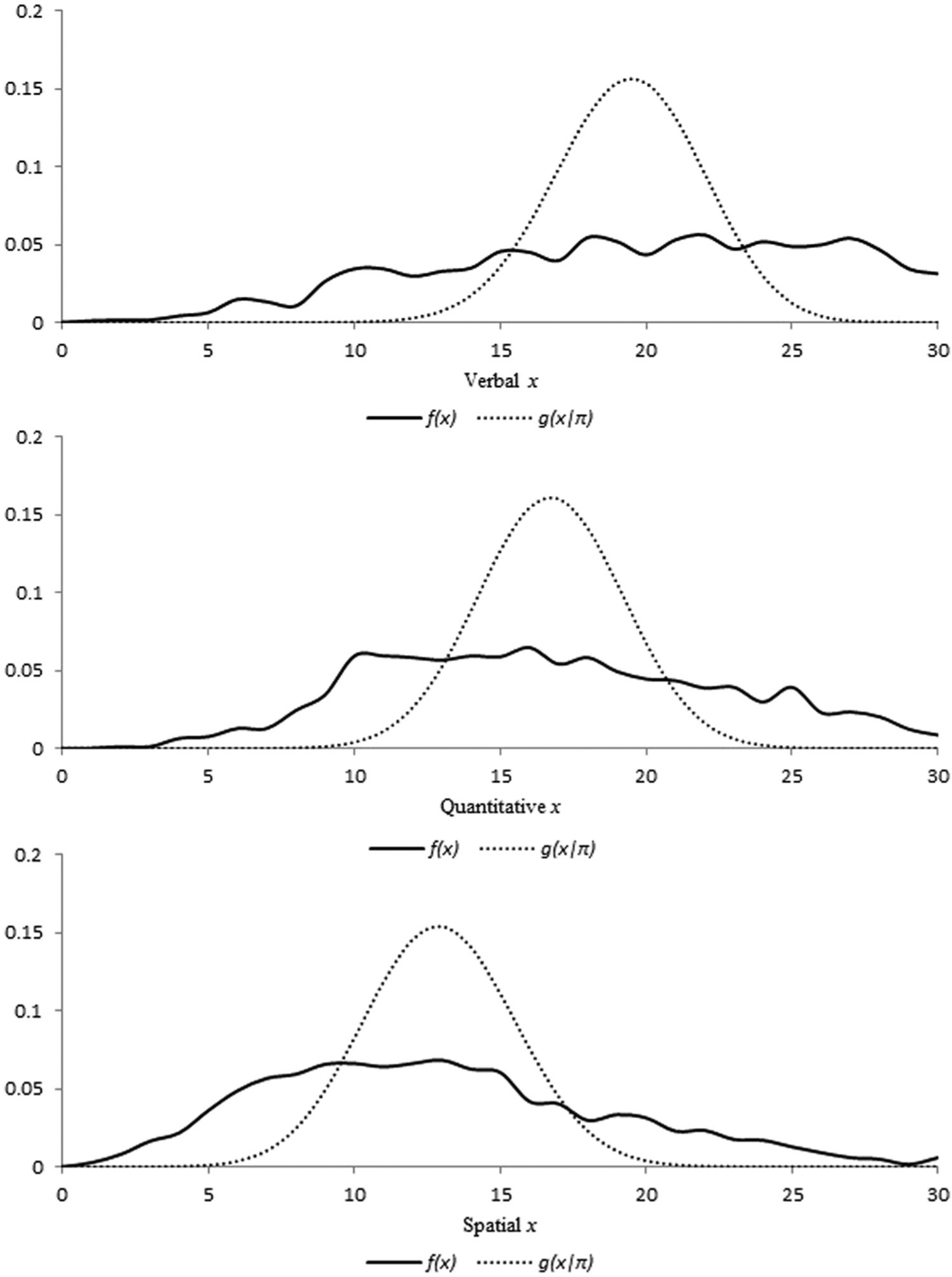
For the three subtests, Figure 1 shows the observed relative frequency distribution of raw scores, $f (x)$ , and conditional distribution of the raw scores given the matrix of observed proportions correct for the items under the assumption of independent item responses and uncorrelated error, $g (x | π)$ . $f (x)$ for the Verbal subtest shows a heavier upper tail (negatively skewed), whereas $f (x)$ for the Spatial and Quantitative subtests show relatively heavier lower tails (positively skewed). However, $g (x | π)$ for the three subtests had an approximately normal shape regardless of the shape of $f (x)$ for the corresponding raw scores.

Figure 1.

Relative observed frequency distribution of raw scores, $f (x)$ , and distribution of raw scores under assumption of independent item responses and uncorrelated error, $g (x | π),$ for the three subtests: Verbal, Quantitative, and Spatial.

The average scores of $g (x | π)$ for the Verbal, Quantitative, and Spatial subtests were estimated and are given in Table 3. These average scores were equal to their corresponding observed average raw scores. Similarly, the average scale scores under $g (x | π)$ were approximately equal to the corresponding observed average scale scores. PR scores were the exception; the average of PR scores under $g (x | π)$ was different from their observed average. Compared with the observed average scores for the three subtests (which were about 50), the average of PR scores under $g (x | π)$ was relatively smaller for the Verbal subtest (47.058) and relatively larger for both the Quantitative subtest (51.432) and Spatial subtest (53.512). This is due to the differences between $f (x)$ and $g (x | π)$ as shown in Figure 1.

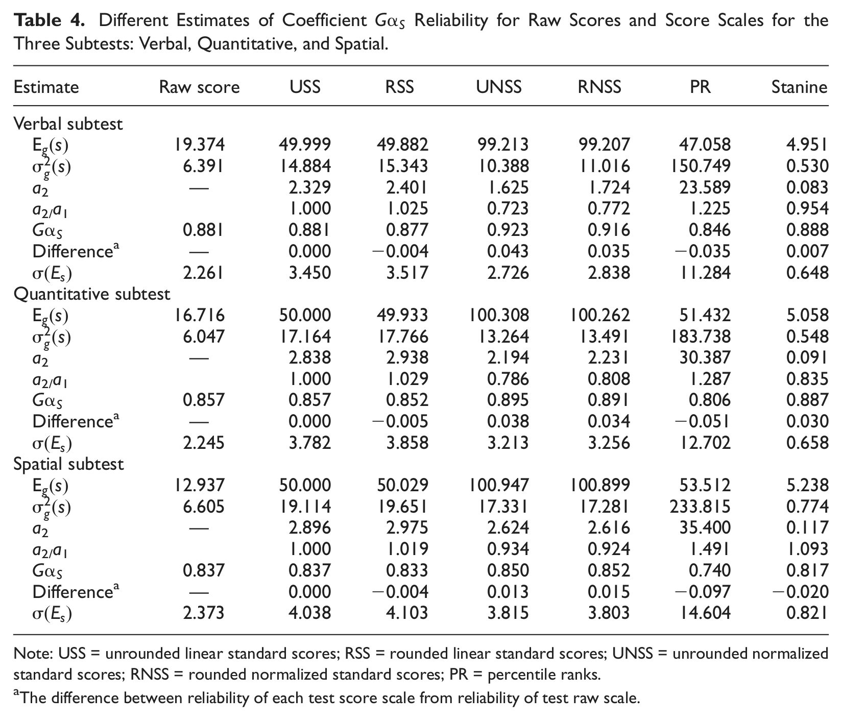
For the three subtests, $σ_{g}^{2} (s)$ were estimated and are presented in Table 4. $σ_{g}^{2} (s)$ are larger for all score scales than for raw scores, except for the stanine scores. The score scales, which have wide score ranges, large standard deviations, and steep slopes, have larger $σ_{g}^{2} (s)$ , whereas stanine scores, which have a relatively narrow score range, a small standard deviation, and a less steep slope, have smaller $σ_{g}^{2} (s)$ . These results reveal that wider and steeper score scales cause larger $σ_{g}^{2} (s)$ , and vice versa. Table 4 also presents the effects ( $a_{2}$ ) of the six transformation functions on $σ_{g}^{2} (s)$ under $g (x | π)$ for the three subtests. As expected, these effects are not equal to $a_{1}$ for the observed scale scores for all the three subtests. This indicates that each transformation function could have different effects on the observed scale score variance and the scale score variance under $g (x | π)$ depending on the distributional shape of $f (x)$ and $g (x | π) .$

Table 4.

Different Estimates of Coefficient $G α_{S}$ Reliability for Raw Scores and Score Scales for the Three Subtests: Verbal, Quantitative, and Spatial.

Estimate	Raw score	USS	RSS	UNSS	RNSS	PR	Stanine
Verbal subtest
$E_{g} (s)$	19.374	49.999	49.882	99.213	99.207	47.058	4.951
$σ_{g}^{2} (s)$	6.391	14.884	15.343	10.388	11.016	150.749	0.530
a₂	—	2.329	2.401	1.625	1.724	23.589	0.083
a₂_/a₁		1.000	1.025	0.723	0.772	1.225	0.954
$G α_{S}$	0.881	0.881	0.877	0.923	0.916	0.846	0.888
Difference^a	—	0.000	−0.004	0.043	0.035	−0.035	0.007
$σ (E_{s})$	2.261	3.450	3.517	2.726	2.838	11.284	0.648
Quantitative subtest
$E_{g} (s)$	16.716	50.000	49.933	100.308	100.262	51.432	5.058
$σ_{g}^{2} (s)$	6.047	17.164	17.766	13.264	13.491	183.738	0.548
a₂	—	2.838	2.938	2.194	2.231	30.387	0.091
a₂_/a₁		1.000	1.029	0.786	0.808	1.287	0.835
$G α_{S}$	0.857	0.857	0.852	0.895	0.891	0.806	0.887
Difference^a	—	0.000	−0.005	0.038	0.034	−0.051	0.030
$σ (E_{s})$	2.245	3.782	3.858	3.213	3.256	12.702	0.658
Spatial subtest
$E_{g} (s)$	12.937	50.000	50.029	100.947	100.899	53.512	5.238
$σ_{g}^{2} (s)$	6.605	19.114	19.651	17.331	17.281	233.815	0.774
a₂	—	2.896	2.975	2.624	2.616	35.400	0.117
a₂_/a₁		1.000	1.019	0.934	0.924	1.491	1.093
$G α_{S}$	0.837	0.837	0.833	0.850	0.852	0.740	0.817
Difference^a	—	0.000	−0.004	0.013	0.015	−0.097	−0.020
$σ (E_{s})$	2.373	4.038	4.103	3.815	3.803	14.604	0.821

Note: USS = unrounded linear standard scores; RSS = rounded linear standard scores; UNSS = unrounded normalized standard scores; RNSS = rounded normalized standard scores; PR = percentile ranks.

The difference between reliability of each test score scale from reliability of test raw scale.

Table 4 also presents coefficient α and $G α_{S}$ of all score scales for the three subtests. Coefficient $G α_{S}$ for each of the six score scales was different for the three subtests. Using α for raw scores as a reference, rows labeled as “difference” in Table 4 provide information about the patterns of increase or decrease in $G α_{S}$ for each of the score scales by computing the arithmetic difference between $G α_{S}$ and α. Coefficient $G α_{S}$ for all score scales showed similar patterns for the three ability subtests. First, $G α_{S}$ for the unrounded linearly transformed scale scores (USS) was equal to α for raw scores. Other nonlinearly transformed scale scores (including rounded linear scale scores, RSS) had different $G α_{S}$ as compared with α for raw scores. $G α_{S}$ for UNSS, RNSS, and stanine scales were relatively larger than α for raw scores for the three subtests, whereas $G α_{S}$ for RSS and PR scores were relatively smaller.

In addition, $G α_{S}$ for some score scales increased, whereas others decreased as compared with α for raw scores with different ability subtests. Relatively, PR scores had the largest amount of decrease in $G α_{S}$ reliability for the three subtests as compared with the other score scales. The Spatial subtest showed the largest decrease in $G α_{S}$ reliability of PR scores as compared with the other ability subtests. However, UNSS and RNSS scores had the largest increases in $G α_{S}$ reliability for the Verbal and the Quantitative subtests. However, stanine scores had the largest increase in $G α_{S}$ reliability for the Spatial subtest. The overall standard errors of measurement were different for different score scales, as displayed in Table 4. In addition, the overall standard error of measurement differed across the three subtests. For the Spatial subtest, for example, they were 2.373, 4.038, 4.103, 3.815, 3.803, 14.604, and 0.821 for raw scores, USS, RSS, UNSS, RNSS, PR, and Stanine, respectively.

Moreover, Table 4 presents the ratio ( $a_{2} / a_{1}$ ) for different score scales to facilitate investigating the relationship between this ratio and change in $G α_{S} .$ Unrounded linearly transformed scores (USS) had a ratio of one and thus had $G α_{S}$ equal to α for raw scores. However, the ratios for the other nonlinearly transformed scales were different from unity. For all the three subtests, UNSS, RNSS, and stanine scores had ratios smaller than unity, and consequently positive differences between $G α_{S}$ and α ( $G α_{S}$ is larger than α). However, RSS and PR scores had ratios larger than unity, and consequently negative differences between their $G α_{S}$ and α ( $G α_{S}$ is smaller than α).

Comparing α and Gα_s With Polytomously Scored Items

This section describes the application of α and $G α_{S}$ to estimate the internal consistency reliability of raw scores and scale scores on polytomously scored items on a noncognitive assessment. The assessment was a self-reporting of Teaching Anxiety.

Sample and Instrument

Teaching Anxiety self-reporting was administered in fall 2009 to a sample of 246 preservice students in their final year at the College of Education. Teaching Anxiety self-reporting aimed to assess participants’ self-reporting of their feelings and tensions while they were experiencing teaching for the first time. The self-reporting consisted of 14 statements that used a 5-point Likert-type rating scale quantifying the frequency of experiencing certain anxiety behaviors as follows: 1 (never), 2 (seldom), 3 (sometimes), 4 (often), and 5 (always). Ten statements in the scale were positively phrased (revealing anxious behaviors), while the remaining four statements were negatively phrased (revealing comfortable behaviors). The responses to the four negatively phrased statements were reversed and added to other statements to obtain the sum of all 14 statements to acquire each participant’s level of teaching anxiety. The score range for raw scores for the Teaching Anxiety self-reporting is between 14 and 70. These raw scores were transformed into two score scales: normalized standard scores (both UNSS and RNSS with a mean of 200 and a standard deviation of 10) and PR scores. In addition, UNSS and RNSS scores were truncated at a scale score of 170 for low raw scores and at 230 for high raw scores. These raw-to-scale transformations were monotonically nondecreasing, nonlinear transformations of raw scores.

Procedure

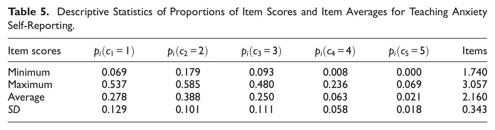
Both coefficient α and $G α_{S}$ were computed for raw scores and score scales of Teaching Anxiety self-reporting, respectively. The proportions for each item score for each of the 14 items were computed and used in the computation of α and $G α_{S} .$ Table 5 presents descriptive statistics for these proportions and item averages. Table 5 shows that the lower item scores ( $c_{1}$ = 1, $c_{2}$ = 2, and $c_{3}$ = 3) had higher proportions than did higher item scores ( $c_{4}$ = 4 and $c_{5}$ = 5). The 14 items had item averages ranging from 1.740 to 3.057, with an overall average of 2.160 and a standard deviation of 0.343.

Table 5.

Descriptive Statistics of Proportions of Item Scores and Item Averages for Teaching Anxiety Self-Reporting.

Item scores	$p_{i} (c_{1} = 1)$	$p_{i} (c_{2} = 2)$	$p_{i} (c_{3} = 3)$	$p_{i} (c_{4} = 4)$	$p_{i} (c_{5} = 5)$	Items
Minimum	0.069	0.179	0.093	0.008	0.000	1.740
Maximum	0.537	0.585	0.480	0.236	0.069	3.057
Average	0.278	0.388	0.250	0.063	0.021	2.160
SD	0.129	0.101	0.111	0.058	0.018	0.343

Results and Discussion

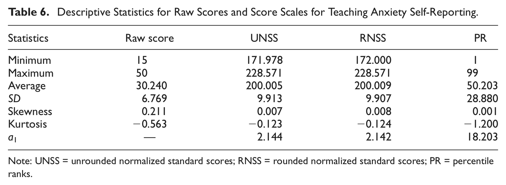
Table 6 shows descriptive statistics for raw scores, UNSS, RNSS, and PR scores for the Teaching Anxiety self-reporting. The observed raw scores ranged between 15 and 50, with an average of 30.24 and a standard deviation of 6.769. No students achieved scores between 50 and 70. Table 6 also presents the effects of transformation functions ( $a_{1}$ ) on the observed variance for each of the score scales. All these effects enlarged the test score variance because of wider score range of these score scales. The largest effects of these transformation functions were observed with UNSS and RNSS.

Table 6.

Descriptive Statistics for Raw Scores and Score Scales for Teaching Anxiety Self-Reporting.

Statistics	Raw score	UNSS	RNSS	PR
Minimum	15	171.978	172.000	1
Maximum	50	228.571	228.571	99
Average	30.240	200.005	200.009	50.203
SD	6.769	9.913	9.907	28.880
Skewness	0.211	0.007	0.008	0.001
Kurtosis	−0.563	−0.123	−0.124	−1.200
a ₁	—	2.144	2.142	18.203

Note: UNSS = unrounded normalized standard scores; RNSS = rounded normalized standard scores; PR = percentile ranks.

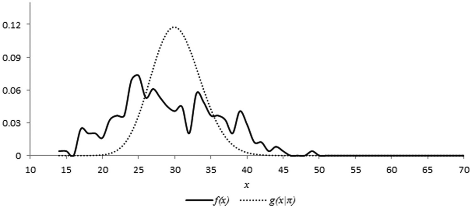
Figure 2 displays $f (x)$ and $g (x | π)$ for raw scores on the Teaching Anxiety self-reporting. $f (x)$ is bumpy and positively skewed. Similar to earlier dichotomously scored items, $g (x | π)$ was approximately normally distributed over all raw scores from 14 to 70. As presented in Table 7, the average raw score under $g (x | π)$ was equal to the observed average raw score. The average scale scores for UNSS, RNSS, and PR scores under $g (x | π)$ were slightly larger than their corresponding observed average scale scores.

Figure 2.

Relative frequency distribution of raw scores, $f (x),$ and conditional distribution of raw scores under assumption of independent item responses and uncorrelated error, $g (x | π),$ for Teaching Anxiety self-reporting.

Table 7.

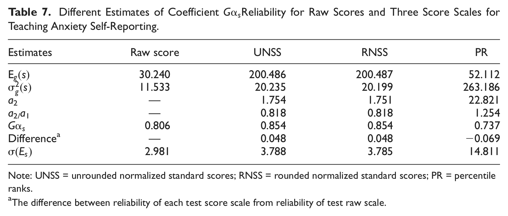
Different Estimates of Coefficient $G α_{s}$ Reliability for Raw Scores and Three Score Scales for Teaching Anxiety Self-Reporting.

Estimates	Raw score	UNSS	RNSS	PR
$E_{g} (s)$	30.240	200.486	200.487	52.112
$σ_{g}^{2} (s)$	11.533	20.235	20.199	263.186
a ₂	—	1.754	1.751	22.821
a ₂ _/a ₁	—	0.818	0.818	1.254
$G α_{s}$	0.806	0.854	0.854	0.737
Difference^a	—	0.048	0.048	−0.069
$σ (E_{s})$	2.981	3.788	3.785	14.811

Note: UNSS = unrounded normalized standard scores; RNSS = rounded normalized standard scores; PR = percentile ranks.

The difference between reliability of each test score scale from reliability of test raw scale.

Table 7 displays scale score variance under $g (x | π)$ , $σ_{g}^{2} (s)$ , for all score scales for the Teaching Anxiety self-reporting. Different score scales had different $σ_{g}^{2} (s)$ . Coefficient $G α_{S}$ reliability for all score scales were different from α for raw scores. Table 7 also presents the difference between $G α_{S}$ and α for all score scales. Coefficient $G α_{S}$ values relatively increased for UNSS scores and RNSS scores, whereas they relatively decreased for PR scores when compared with α for raw scores. The overall standard errors of measurement were different for different score scales as displayed in Table 7. They were 2.981, 3.788, 3.785, and 14.811 for raw scores, UNSS, RNSS, and PR, respectively.

Table 7 also presents the ratio ( $a_{2} / a_{1}$ ) of the two effects of the three transformation functions for the different score scales. This ratio effect was different for the different score scales. UNSS and RNSS scores had ratios smaller than unity, and consequently, positive differences between their $G α_{S}$ and α for raw scores ( $G α_{S}$ is larger than α). However, PR scores had a ratio larger than unity and consequently, negative differences between their $G α_{S}$ and α values ( $G α_{S}$ is smaller than α).

Summary and Conclusion

It is important to investigate not only how reliable raw scores are but also how reliable the scale scores resulting from a nonlinear transformation of raw scores are. This is because scale scores are the scores used for interpreting test results for both individual examinees and decision makers (American Educational Research Association, American Psychological Association, & National Council on Measurement in Education, 1999). This article presents coefficient α in a generalized form, $G α_{S},$ allowing for its use to estimate reliability of scale scores. If raw scores are transformed using a linear transformation, $G α_{S}$ reduces to α.

Estimating $G α_{S}$ reliability for scale scores requires three pieces of information: (a) the observed proportions of all possible scores on each item from sampled data, (b) the observed relative frequency distribution of raw scores, $f (x)$ , and (c) the raw-to-scale transformation table. A recursive formula (Equations 16 and 17) is implemented to obtain the conditional distribution of raw scores given the matrix of observed proportions of all possible item scores under the assumption of independent item responses and uncorrelated error scores, $g (x | π)$ . This $g (x | π)$ and the raw-to-scale transformation table are then used to estimate the scale score variance, $σ_{g}^{2} (s)$ (Equation 11). Similarly, $f (x)$ and the raw-to-scale transformation table are used to obtain the observed scale score variance, $σ^{2} (s)$ (Equation 13). Finally, these two variances are substituted into Equation 14 to estimate $G α_{S} .$

$G α_{S}$ for scale scores gives coefficient KR-20-type reliability with dichotomously scored items and coefficient α-type reliability with polytomously scored items. $G α_{S}$ can be used to estimate the reliability of any type of score scales that incorporates relative-based process and relative decision. $G α_{S}$ assumes essentially tau-eq24 test forms similar to α with no other assumptions about either true scores or error scores.

Moreover, all raised interpretations, uses, and misuses of α (e.g., Bentler, 2009; Cortina, 1993; Cronbach, 1951; Graham, 2006; Hensen, 2001; Miller, 1995; Rodriguez & Maeda, 2006; Schmitt, 1996; Sijtsma, 2009) are applicable to $G α_{S} .$ For example, coefficient α is known to be a lower bound of reliability if the assumption of essentially tau-equivalent test forms is violated. Similarly, this also applies to $G α_{S} .$ In addition, both α and $G α_{S}$ assume uncorrelated error scores, which was criticized by a number of researchers (e.g., Green & Hershberger, 2000; Green & Yang, 2009; Raykov, 1998). If the assumption of uncorrelated error scores is violated with test data, neither coefficient α nor $G α_{S}$ should be used to estimate reliability of test scores. Methods that incorporate structural equation modeling could be used instead (Green & Yang, 2009).

The conditional distribution of raw scores under the assumption of independent item responses and uncorrelated error scores, $g (x | π),$ gives different information from the information given by the observed distribution of raw scores, $f (x) .$ $g (x | π)$ gives the conditional distribution of raw scores assuming there were no commonalities among test items. It helps to estimate the scale score variance under $g (x | π),$ which equals the sum of item variances required in the typical formula of coefficient α. $g (x | π)$ is computed conditionally on the proportions of possible item scores observed with a sample of examinees. However, the observed relative distribution of raw scores, $f (x),$ gives the distribution of raw scores when items covary with each other and are intercorrelated. $f (x)$ is gathered from the administration of test items to a sample of examinees. It helps to estimate the observed scale score variance. The extent to which the observed scale score variance is larger than the scale score variance under $g (x | π)$ determines the reliability level of raw/scale scores. As Kuder and Richardson (1937) argued, “reliability is the characteristic of a test possessed by virtue of the positive intercorrelations of the items composing it” (p. 159).

The application of $G α_{S}$ to different data sets with dichotomously scored and polytomously scored items showed that different score scales might have different scale score variances under $g (x | π)$ and $G α_{S}$ reliability. The resulting reliability for scale scores might be either higher or lower than the reliability for raw scores. For example, with all data sets in this study, normalized standard scores (UNSS and RNSS) and Stanine showed an increase in test score reliability. However, PR scores showed a decrease in test score reliability. Although the PR scale is one of the most commonly used scales for score interpretation, the results of all data sets in this article suggested that PR scale showed lower $G α_{S}$ reliability than raw scores and other score scales. This could be explained by the process of formulating PR scores, as explained earlier. This result about PR scores, however, should not be generalized to PR scores for other data sets.

Moreover, the results showed that the magnitudes of increase or decrease in test score reliability were different for different score scales. The effects of a transformation function on the scale score variance, $σ_{g}^{2} (s)$ , for each score scale differ from its effect on the observed scale score variance, $σ^{2} (s)$ . The direction of the effect of the transformation function on $G α_{S}$ is predictable (either increasing or decreasing) based on the ratio of the effect of the used transformation function but with an unpredictable magnitude. $σ_{g}^{2} (s)$ is directly influenced by $g (x | π)$ and the raw-to-scale transformation function. $σ^{2} (s)$ is directly influenced by $f (x)$ and the raw-to-scale transformation function.

As demonstrated in Equation 19, the reliability of scale scores is smaller than the reliability of raw scores if the average effect of the transformation function on the test score variance under $g (x | π)$ is larger than on the observed raw score variance under $f (x)$ ( $a_{2} > a_{1}$ ), and vice versa. The ratio $(a_{2} / a_{1}$ ) determines the increase or decrease in the reliability of scale scores relative to the reliability of raw scores. Whenever this ratio goes farther from unity, the amount of the effect of a transformation function on the reliability of test scores (either increasing or decreasing) becomes larger (more or less), and vice versa. Hence, the interaction among $f (x)$ , $g (x | π)$ , and a raw-to-scale transformation function could introduce extra sources of measurement error or could reduce the existing measurement error in measuring a person’s trait. How different score scales affect measurement error and reliability of test scores deserves a thorough investigation by future researchers.

In this study, only coefficient $G α_{S}$ reliability for some score scales that are used to provide normative information (PR, standard scores, stanine) were studied. However, $G α_{S}$ can be applied to estimate the reliability for other transformed scores resulting from equating, regression, and prediction analyses. Score scales resulting from these transformation functions might have different patterns of $G α_{S}$ from those discussed in this article. Future studies applying $G α_{S}$ and investigating its behavior with these transformed scores are strongly recommended.

One of the most important criteria for choosing an appropriate test score scale is whether it is elevating or at least maintaining the current level of reliability achieved by raw scores. $G α_{S}$ provides a general way that can be used to investigate whether a selected score scale preserves, improves, or weakens the achieved reliability of raw scores. Results of this study showed that nonlinearly transformed scores yielded either a higher or lower reliability than did linearly transformed scores (equal to the reliability of raw scores) for the same data. This result suggests that linearly transformed scores might be preferred over nonlinearly transformed scores if the latter showed a lower reliability than the reliability for raw scores. Linearly transformed scores require relatively simple methods to construct and may provide easier interpretation. However, nonlinearly transformed scores with a lower reliability could be used if they are shown to improve test score validity.

In summary, coefficient $G α_{S}$ does give an estimate of the internal consistency reliability for scale scores that incorporate a normative-based process to assign the scale scores. In other words, $G α_{S}$ examines the extent to which the implemented score scale ensures reliable and consistent interpretation and usage of test results. Since $G α_{S}$ is a general form of α, all issues, uses, and misuses of α are applicable also to $G α_{S} .$ Moreover, new issues and misuses related to the type of score scales might be raised with $G α_{S}$ . Future studies are highly recommended to investigate new issues with $G α_{S}$ for different types of score scales.

Footnotes

Acknowledgements

I thank the editor and the two anonymous reviewers for their insightful comments that helped in the presentation of the article. I am grateful to the Bureau of Education for the Gulf States for providing data.

Declaration of Conflicting Interests

The author declared no potential conflicts of interest with respect to the research, authorship, and/or publication of this article.

Funding

The author received no financial support for the research, authorship, and/or publication of this article.

References

American Educational Research Association, American Psychological Association, & National Council on Measurement in Education. (1999). Standards for educational and psychological testing. Washington, DC: Author.

Bentler

P. M.

(2009). Alpha, dimension-free, and model-based internal consistency reliability. Psychometrika, 74, 137-143.

Brennan

R. L.

(2001). Generalizability theory. New York, NY: Springer.

Brennan

R. L.

Lee

(1999). Conditional scale-score standard error of measurement under binomial and compound binomial assumptions. Educational and Psychological Measurement, 59, 8-24.

Cortina

J. M.

(1993). What is coefficient alpha? An examination of theory and applications. Journal of Applied Psychology, 78, 98-104.

Cronbach

L. J.

(1951). Coefficient alpha and the internal structure of tests. Psychometrika, 16, 297-334.

Cronbach

L. J.

Gleser

G. C.

Nanda

Rajaratnam

(1972). The dependability of behavioral measurements: Theory of generalizability for scores and profiles. New York, NY: Wiley.

Cronbach

L. J.

Shavelson

R. J.

(2004). My current thoughts on coefficient alpha and successor procedures. Educational and Psychological Measurement, 64, 391-418.

Feldt

L. S.

(1984). Some relationships between the binomial error model and classical test theory. Educational and Psychological Measurement, 44, 883-891.

10.

Feldt

L. S.

Brennan

R. L.

(1989). Reliability. In Linn

R. L.

(Ed.), Educational measurement (3rd ed., pp. 105-146). New York, NY: Macmillan.

11.

Feldt

L. S.

Qualls

A. L.

(1998). Approximating scaled score standard error of measurement from the raw score standard error. Applied Measurement in Education, 11, 159-177.

12.

Graham

J. M.

(2006). Congeneric and (essentially) tau-equivalent estimates of core reliability: What they are and how to use them. Educational and Psychological Measurement, 66, 930-944.

13.

Green

S. B.

Hershberger

S. L.

(2000). Correlated errors in true score models and their effect on coefficient alpha. Structural Equation Modeling, 7, 251-270.

14.

Green

S. B.

Yang

(2009). Commentary on coefficient alpha: A cautionary tale. Psychometrika, 74, 121-135.

15.

Guttman

(1945). A basis for analyzing test-retest reliability. Psychometrika, 10, 255-282.

16.

Hanson

B. A.

(1994). Extension of Lord-Wingersky algorithm to computing tests scores for polytomous items. Unpublished manuscript, ACT, Iowa City, IA.

17.

Hensen

R. K.

(2001). Understanding internal consistency reliability estimates. Measurement and evaluation in counseling and development, 34, 177-189.

18.

Hoyt

(1941). Test reliability estimated by analysis of variance. Psychometrika, 6, 153-160.

19.

Kolen

M. J.

Hanson

B. A.

Brennan

R. L.

(1992). Conditional standard errors of measurement for scale scores. Journal of Educational Measurement, 29, 285-307.

20.

Kolen

M. J.

Lee

(2011). Psychometric properties of raw and scaled scores on mixed-format tests. Educational Measurement: Issues and Practice, 30, 15-24.

21.

Kolen

M. J.

Wang

Lee

(2012). Conditional standard errors of measurement for composite scores using IRT. International Journal of Testing, 12, 1-20.

22.

Kolen

M. J.

Zeng

Hanson

B. A.

(1996). Conditional standard errors of measurement for scaled scores using IRT. Journal of Educational Measurement, 33, 129-140.

23.

Kuder

G. F.

Richardson

M. W.

(1937). The theory of the estimation of test reliability. Psychometrika, 2, 151-160.

24.

Lee

(2007). Multinomial and compound Multinomial error models for tests with complex item scoring. Applied Psychological Measurement, 31, 255-274.

25.

Lee

Brennan

R. L.

Kolen

M. J.

(2000). Estimators of conditional scale-score standard error of measurement: A simulation study. Journal of Educational Measurement, 37, 1-20.

26.

Lord

F. M.

(1965). A strong true-score theory with application. Psychometrika, 30, 239-270.

27.

Lord

F. M.

Wingersky

M. S.

(1984). Comparison of IRT true-score and equipercentile observed-score “equatings.” Applied Psychological Measurement, 8, 453-461.

28.

Miller

M. B.

(1995). Coefficient alpha: A basic introduction from the perspectives of classical test theory and structural equation modeling. Structural Equation Modeling, 2, 255-273.

29.

Petersen

N. S.

Kolen

M. J.

Hoover

H. D.

(1989). Scaling, norming, and equating. In Linn

R. L.

(Ed.), Educational measurement (3rd ed., pp. 221-262). New York, NY: Macmillan.

30.

Raykov

(1998). Coefficient alpha and composite reliability with interrelated nonhomogeneous items. Applied Psychological Measurement, 22, 375-385.

31.

Rodriguez

M. C.

Maeda

(2006). Meta-analysis of coefficient alpha. Psychological Methods, 11, 306-322.

32.

Schmitt

(1996). Uses and abuses of coefficient alpha. Psychological Assessment, 4, 350-353.

33.

Sijtsma

(2009). On the use, the misuse, and the very limited usefulness of Cronbach’s alpha. Psychometrika, 74, 107-120.

34.

Thissen

Pommerich

Billeaud

Williams

V. S.

(1995). Item response theory for scores on tests including polytomous items with ordered responses. Applied Psychological Measurement, 19, 39-49.

35.

Tong

Kolen

M. J.

(2006). Scaling: An ITEMS module. Educational Measurement: Issues and Practice, 29, 39-48.

36.

Wang

Kolen

M. J.

Harris

D. J.

(2000). Psychometric properties of scaled scores and performance levels for performance assessments using polytomous IRT. Journal of Educational Measurement, 37, 141-162.

Coefficient Alpha and Reliability of Scale Scores

Abstract

Keywords

Coefficient α

Different Forms of Coefficient α

Coefficient Generalized α Reliability for Scale Scores, Gα s

General Method to Obtain g(x|π)

Effect of Transformation Function on Reliability of Test Scores

Comparing α and Gα s With Dichotomously Scored Items

Sample and Instrument

Procedure

Results and Discussion

Comparing α and Gα s With Polytomously Scored Items

Sample and Instrument

Procedure

Results and Discussion

Summary and Conclusion

Footnotes

Acknowledgements

Declaration of Conflicting Interests

Funding

References

Coefficient Generalized α Reliability for Scale Scores, Gα_s

Comparing α and Gα_s With Dichotomously Scored Items

Comparing α and Gα_s With Polytomously Scored Items