Statistical Refinement of the Q-Matrix in Cognitive Diagnosis

Abstract

Most methods for fitting cognitive diagnosis models to educational test data and assigning examinees to proficiency classes require the Q-matrix that associates each item in a test with the cognitive skills (attributes) needed to answer it correctly. In most cases, the Q-matrix is not known but is constructed from the (fallible) judgments of experts in the educational domain. It is widely recognized that a misspecification of the Q-matrix can negatively affect the estimation of the model parameters, which may then result in the misclassification of examinees. This article develops a Q-matrix refinement method based on the nonparametric classification method (Chiu & Douglas, in press), and comparisons of the residual sum of squares computed from the observed and the ideal item responses. The method is evaluated with three simulation studies and an application to real data. Results show that the method can identify and correct misspecified entries in the Q-matrix, thereby improving its accuracy.

Keywords

classification cognitive diagnosis Q-matrix residual sum of squares validity

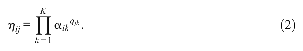
Cognitive diagnosis models of educational test performance decompose overall ability in the domain of the test into a set of specific skills, called “attributes,” that an examinee may or may not possess, thereby providing a detailed description, or “attribute pattern,” of his or her strengths and weaknesses in the domain. The entire set of possible attribute patterns for a given test defines proficiency classes to which examinees can be assigned. Model-based methods use maximum likelihood estimation (MLE) procedures to estimate model parameters that are then used to assign examinees to proficiency classes (de la Torre, 2008, 2009, 2011; de la Torre & Douglas, 2008; Haertel, 1989; Hartz, Roussos, Henson, & Templin, 2005; Henson, Templin, & Willse, 2009; Junker & Sijtsma, 2001; Maris, 1999; Tatsuoka, 1990; Tatsuoka & Tatsuoka, 1987, 1997; von Davier, 2005). Nonmodel-based methods use statistical clustering techniques, such as cluster analysis, to achieve classification without model fitting (Ayers, Nugent, & Dean, 2008; Chiu & Douglas, 2013; Chiu, Douglas, & Li, 2009; Chiu & Seo, 2009). Both approaches require that the Q-matrix (Tatsuoka, 1985) underlying a given test be known. The binary J×K Q-matrix indicates whether test item j, j = 1,…,J, requires that an examinee possess attribute k, k = 1,…,K, to respond correctly to that item. Each “q-entry,”q_jk, of the Q-matrix is coded 0 (not required) or 1 (required). Each row or “q-vector,” q _j, of the Q-matrix thus specifies all attributes that an examinee must possess for a correct response to item j. For a test measuring K attributes, there are 2^K possible attribute patterns and hence, 2^K proficiency classes.

Unfortunately, the Q-matrix for most educational tests is not known, so the (fallible) judgment of experts in the domain of the test is used to establish the associations between the test items and the attributes, risking a misspecified Q-matrix. It is widely recognized (e.g., de la Torre, 2008; de la Torre & Chiu, 2010; Rupp & Templin, 2008) that a misspecified Q-matrix can negatively affect the estimation of the model parameters, which may then result in the misclassification of examinees, but little research into methods for detecting and correcting a misspecified Q-matrix has been conducted.

Recently, however, de la Torre (2008) proposed a model-based method for Q-matrix validation based on an item discrimination index, ϕ_j, that maximizes the difference in the probabilities of a correct response to item j between examinees who possess all the attributes required for a correct response to that item and examinees who do not, for observed item responses conforming to the Deterministic Input, Noisy Output, “And” gate (DINA) model (Junker & Sijtsma, 2001; Macready & Dayton, 1977). The performance of this method was evaluated with a simulation study and two applications to real data sets. The simulation study demonstrated that the method was able to identify and replace the misspecified q-vectors and retain the correct q-vectors in the Q-matrix. Although this method appeared promising, it was not justified theoretically; the simulation study evaluated its performance for only a fixed number of test items, attributes, and examinees, and a single level of error perturbation of the observed item responses; and it is not known whether the method can be used when observed item responses conform to models other than the DINA model.

Accordingly, de la Torre and Chiu (2010) proposed another item discrimination index, $ς_{j}^{2}$ , to be used for Q-matrix validation when the observed item responses conform to the Generalized DINA (G-DINA) model (de la Torre, 2011). The method based on this index corrects a misspecified q-vector one misspecified q-entry at a time, whereas de la Torre’s (2008) method replaces an entire misspecified q-vector with the correct q-vector. De la Torre and Chiu (2010) provided a thorough mathematical justification for their method; a simulation study demonstrated that their method can accurately identify and replace the misspecified q-entries while retaining the correct q-entries. Again, however, the simulation study was limited in scope and did not vary the number of test items, attributes, or examinees, and so the robustness of the method could not be assessed.

DeCarlo (2012) proposed a Bayesian model-based method for Q-matrix validation when the data conform to the R-DINA model, a reparameterization of the DINA model. DeCarlo’s method requires that the possibly misspecified entries in the Q-matrix be identified in advance. They are treated as random variables and estimated simultaneously with the other parameters in the model using OpenBUGS. The method was tested in the simulation studies with positive results. But as DeCarlo cautioned, further studies are needed to assess the robustness and generalizability of the method.

Although the development of model-based methods for Q-matrix validation is ongoing, the MLE procedures on which they are based often encounter difficulties in practice. For example, the technical complexity of these procedures means that sophisticated, high-quality software is necessary; such software tends to be proprietary and so either unavailable to educational practitioners or expensive to obtain. Moreover, the technical complexity of these procedures may seem overwhelming if the application involves only simple data screening or the resolution of ambiguities in the Q-matrix. MLE procedures also require large numbers of examinees that may not be available in small or medium-sized testing programs, are iterative procedures that are sensitive to starting values, and do not guarantee optimal solutions despite often consuming considerable amounts of computer time.

Some researchers have attempted to develop nonparametric methods of Q-matrix validation that do not rely on the estimation of model parameters. Problems encountered in the development of these methods include ambiguities in determining the attributes needed to respond correctly to test items, and, as was the case for the model-based methods, heavy computational burdens. For example, the hill-climbing algorithm proposed by Barnes (2010) attempted to reconstruct the Q-matrix of a test directly from examinees’ observed item responses. Unfortunately, the algorithm often terminates with the estimated q-entries having values between 0 and 1, limiting the usefulness of the estimated Q-matrix for cognitive diagnosis. Liu, Xu, and Ying (2012) developed an algorithm to estimate the Q-matrix by minimizing a loss function and proved that the estimated Q-matrix converges to the true Q-matrix as the number of examinees goes to infinity, given some assumptions. The loss criterion is a function of the entire Q-matrix, so the algorithm may require evaluating all possible 2^KJ Q-matrices, which is not computationally feasible for tests that have more than a few items requiring possession of more than a few attributes for a correct response.

This article develops a new method, the Q-matrix refinement method, for identifying and correcting the misspecified q-entries of a Q-matrix. The method operates by minimizing the residual sum of squares (RSS) between the observed responses and the ideal responses to a test item. The method takes into account the limitations of the few existing methods for validating a Q-matrix, is theoretically justified, can be implemented in readily available statistical packages, does not rely on the estimation of model parameters, and makes no assumptions other than those made by the cognitive diagnosis model supposed to underlie examinees’ observed item responses. Presentation of the Q-matrix refinement method begins with an overview of the two cognitive diagnosis models under consideration and a description of the nonparametric classification method (Chiu & Douglas, 2013) used by the Q-matrix refinement method algorithm to estimate examinees’ proficiency-class memberships. The next section provides a theoretical justification of the Q-matrix refinement method and describes the algorithm developed on the basis of that justification. The performance of the method is then evaluated under a wide range of conditions with three simulation studies and an application to real data. Finally, the discussion addresses an issue raised by the results of the simulation studies, suggests directions for future research, and comments on the advantages of the method.

Overview of Cognitive Diagnosis Models and the Nonparametric Classification Method

The two cognitive diagnosis models—the DINA model and the Noisy Input, Deterministic Output, “And” gate (NIDA) model—under consideration here both require the specification of a J×K Q-matrix, where J is the number of test items and K is the number of attributes. These models differ only in the way that examinees are assumed to use their attributes to respond to the items. Let the ith examinee’s attribute pattern α_i be a K-dimensional vector where the kth entry, $α_{ik}$ , indicates nonpossession (0) or possession (1) of attribute k, where k = 1, 2,…,K. Also, let Y_ij be the observed response (0 = incorrect, 1 = correct) of examinee i to item j. The item response function of the DINA model is

P (Y_{i j} = 1 | α_{i}) = {(1 - s_{j})}^{η_{i j}} {g_{j}}^{(1 - η_{i j})},

where $s_{j} = P (Y_{i j} = 0 | η_{i j} = 1)$ and $g_{j} = P (Y_{i j} = 1 | η_{i j} = 0)$ are the probabilities of slipping (failing to answer the item correctly despite having the skills required to do so) and guessing (answering the item correctly despite lacking the skills required to do so), respectively. Parameter $η_{ij}$ is the ideal item response that associates the attributes possessed by examinee i with the q-entries of item j:

η_{ij} = Π_{k = 1}^{K} {α_{ik}}^{q_{jk}} .

The ideal item response $η_{ij}$ indicates whether examinee i possesses all the attributes needed for answering item j correctly, and the DINA model is thus a conjunctive model.

The NIDA model, introduced by Maris (1999) and named by Junker and Sijtsma (2001), differs from the DINA model in that it defines slipping and guessing parameters at the attribute level rather than at the item level. Let $η_{ijk}$ indicate whether examinee i correctly applied the kth attribute in responding to item j; then the slipping and guessing parameters are $s_{k} = P (η_{i j k} = 0 | α_{i k} = 1, q_{i k} = 1)$ and $g_{k} = P (η_{i j k} = 1 | α_{i k} = 0, q_{i k} = 1),$ respectively. The item response function of the NIDA model is

P (Y_{i j} = 1 | α_{i}) = \prod_{k = 1}^{K} {[{(1 - s_{k})}^{α_{i k}} {g_{k}}^{(1 - α_{i k})}]}^{q_{j k}} .

The NIDA model is somewhat restrictive because it implies that the item response function must be the same for each item requiring possession of the same attributes for a correct response. That item difficulty must be exactly the same for many items in a test is not a realistic expectation. The item response function for the generalized NIDA model that allows the slipping and guessing parameters to differ from item to item is

P (Y_{i j} = 1 | α_{i}) = \prod_{k = 1}^{K} {[{(1 - s_{k})}^{α_{i k}} {g_{jk}}^{(1 - α_{i k})}]}^{q_{j k}} .

The DINA model and the generalized NIDA model are used in the simulation studies presented later to generate observed item responses to be used in evaluating the performance of the Q-matrix refinement method. However, the method does not require actually fitting these models. Instead, it adopts the nonparametric classification method (Chiu & Douglas, 2013) to classify examinees according to their attribute patterns, which are determined by comparing their observed item response patterns to their ideal item response patterns. The class membership of an examinee is estimated by minimizing the distance between the observed item response pattern and all possible ideal item response patterns. More specifically, let $η_{i} = η_{i 1},\dots, η_{i J}$ ) represent the ideal item response pattern of examinee i, where $η_{ij}$ is the ideal item response to item j as defined in Equation 2. It is clear that $η_{i}$ depends only on the Q-matrix and is a function of the unobservable α_i. Therefore, there are 2^K ideal item response patterns, $η^{(1)}, η^{(2)}, \dots, η^{(2^{K})}$ , each of which corresponds to one of the 2^K possible attribute patterns. The problem of obtaining an estimated attribute pattern, ${\hat{α}}_{i}$ for examinee i amounts to minimizing the distance between the observed and the possible ideal item response patterns, $d (y_{i}, η^{(m)}),$ for m = 1, 2, …,M = 2^K. That is, ${\hat{α}}_{i}$ is the attribute pattern that gives an ideal item response pattern, from all possible such patterns, that is the closest (most similar) to the observed item response pattern $y_{i} .$

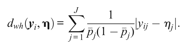
For binary data, a very natural and frequently used distance measure is the Hamming distance, which simply counts the number of times that the entries in two vectors differ. Here, a weighted version of the Hamming distance is used to accommodate item variability. Let ${\bar{p}}_{j}$ be the proportion of examinees responding correctly to item j. Then the weighted Hamming distance is

d_{w h} (y_{i}, η) = \sum_{j = 1}^{J} \frac{1}{{\bar{p}}_{j} (1 - {\bar{p}}_{j})} | y_{i j} - η_{j} | .

Chiu and Douglas (2013) described several desirable features of the nonparametric classification method. First, the method does not require much computer time but nonetheless yields classification rates almost as high as those of the parametric model-based methods that use MLE to obtain the item parameters that are then used to classify examinees. This is so even when the sizes of the item parameters are unreasonably large (e.g., s and g equal to 0.5) and/or when correct responses to the items require possession of a large number of attributes (e.g., K equals 8). Second, the method can be employed with observed item responses that conform to any cognitive diagnosis model that uses an ideal item response to link the q-entries of an item with the attributes possessed by an examinee. This flexibility guarantees good examinee classification even when the true model underlying the observed item responses is unknown. Third, when the Q-matrix has been misspecified, the method can identify examinees’ attribute patterns almost as well as, or even better than, the model-based methods when the true underlying model has been used. Because of its effectiveness, efficiency, and robustness, the nonparametric classification method for estimating examinees’ class memberships has been incorporated into the Q-matrix refinement method.

Q-Matrix Refinement Method

This section provides a justification for the Q-matrix refinement method and describes the algorithm developed on the basis of that justification. The algorithm operates by minimizing the RSS computed from the observed response and the ideal response to each test item. Recall that Y_ij and $η_{ij}$ are the observed and ideal item responses of examinee i to item j, respectively. Then the RSS of item j for examinee i is defined as

R S S_{i j} = {(Y_{i j} - η_{i j})}^{2} .

The RSS of item j across all examinees is therefore

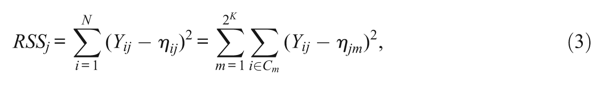
R S S_{j} = \sum_{i = 1}^{N} {(Y_{i j} - η_{i j})}^{2} = \sum_{m = 1}^{2^{K}} \sum_{i \in C_{m}} {(Y_{i j} - η_{i j m})}^{2},

where C_m is the latent proficiency-class m, and N is the number of examinees. Note that the index of the ideal response to item j has changed from “ij” to “jm” because ideal item responses are class-specific; that is, every examinee in the same class has the same ideal response to an item. The use of RSS as a loss function to identify the misspecified q-vector for an item is based on the notion that the RSS of the correct q-vector is expected to be the lowest RSS of all the possible q-vectors, given a correct classification of examinees. Because the RSS of each item is independent of the RSS of every other item, the overall RSS of the test will also be minimized as the misspecified q-vectors are corrected.

Justification

The Q-matrix refinement method is justified by demonstrating that the RSS of the correct q-vector for an item is less than the RSS of each misspecified q-vector for that item, given a correct classification of examinees. Let $α_{m} = (α_{m 1}, α_{m 2},\dots, α_{m K})$ be the K-dimensional attribute pattern of the examinees in class m and $q_{j} = (q_{j 1},\dots, q_{jK})$ be the correct q-vector of item j. Assuming that the observed item responses conform to the DINA model, the item response function in Equation 1 can be rewritten in terms of the attribute pattern α_m associated with class m as

P (Y_{j} = 1 | α_{m}) = {(1 - s_{j})}^{η_{j m}} {g_{j}}^{(1 - η_{j m})},

where $η_{j m} = η_{j} (α_{m}) = \prod_{k = 1}^{k} {α_{m k}}^{q_{j k}}$ is a function of α_m. The conditional expectation of the observed response to item j, given α_m, is then

E (Y_{j} | α_{m}) = {(1 - s_{j})}^{η_{j m}} {g_{j}}^{(1 - η_{j m})} .

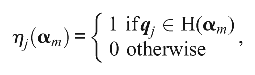
Next, let H(α) = {α_l|α_l is nested within α}, where “nested” means that the attributes present in α_l are a subset of those present in α. Accordingly, $η_{jm}$ can be re-expressed as

η_{j} (α_{m}) = {\begin{matrix} 1 if q_{j} \in H (α_{m}) \\ 0 otherwise \end{matrix},

which leads to

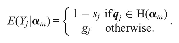
E (Y_{j} | α_{m}) = {\begin{matrix} 1 - s_{j} \\ g_{j} \end{matrix} \begin{matrix} if q_{j} \in H (α_{m}) \\ otherwise . \end{matrix} .

The absolute difference between an observed item response and its corresponding ideal item response, given an attribute pattern α_m, equals

E (| Y_{j} - η_{j} | | α_{m}) = {\begin{matrix} s_{j} \\ g_{j} \end{matrix} \begin{matrix} if q_{j} \in H (α_{m}) \\ otherwise \end{matrix} .

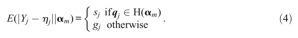
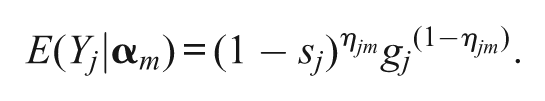
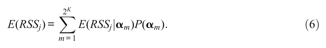
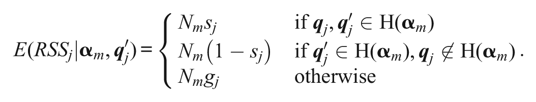
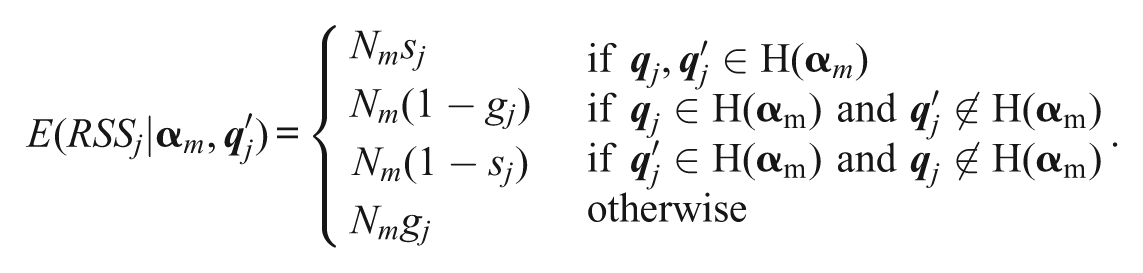
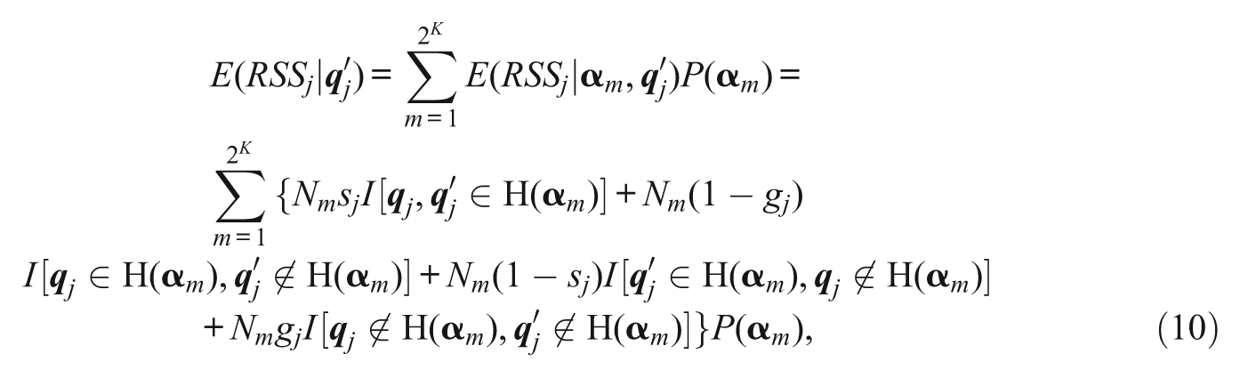
Note that the index “m” has been dropped from $η_{jm}$ to avoid the redundancy due to the conditioning on α_m.

Based on Equation 3, the conditional expectation of the RSS of item j, given attribute pattern α_m, is

\begin{matrix} E (R S S_{j} | α_{m}) = E (\sum_{i \in C_{m}} {(Y_{i j} - η_{j})}^{2} | α_{m}) \\ = E (\sum_{i \in C_{m}} | Y_{i j} - η_{j} | | α_{m}) \\ = \sum_{i \in C_{m}} E (| Y_{i j} - η_{j} | | α_{m}) \\ = N_{m} E (| Y_{j} - η_{j} | | α_{m}) \end{matrix},

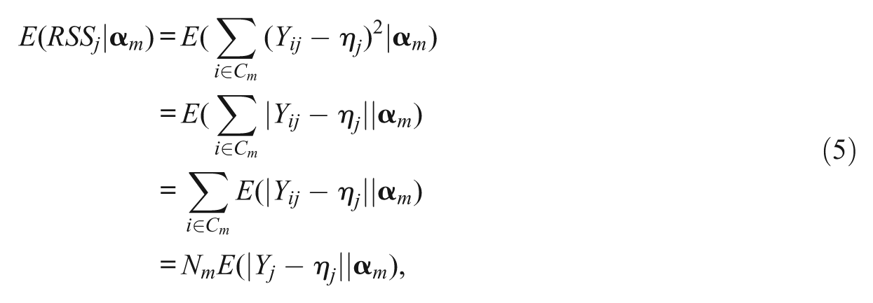
where N_m represents the number of examinees in class m. Then, combining Equation 5 with the definition of the expectation of a discrete random variable gives

E (R S S_{j}) = \sum_{m = 1}^{2^{K}} E (R S S_{j} | α_{m}) P (α_{m}) .

So, $E (RS S_{j})$ can be determined from $E (R S S_{j} | α_{m}),$ provided that $P (α_{m})$ is known.

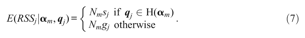
Given the correct q-vector for item j, $q_{j}$ , Equation 4 allows Equation 5 to be elaborated as

E (R S S_{j} | α_{m}, q_{j}) = {\begin{matrix} N_{m} s_{j} \\ N_{m} g_{j} \end{matrix} \begin{matrix} if q_{j} \in H (α_{m}) \\ otherwise \end{matrix} .

Equation 6 then becomes

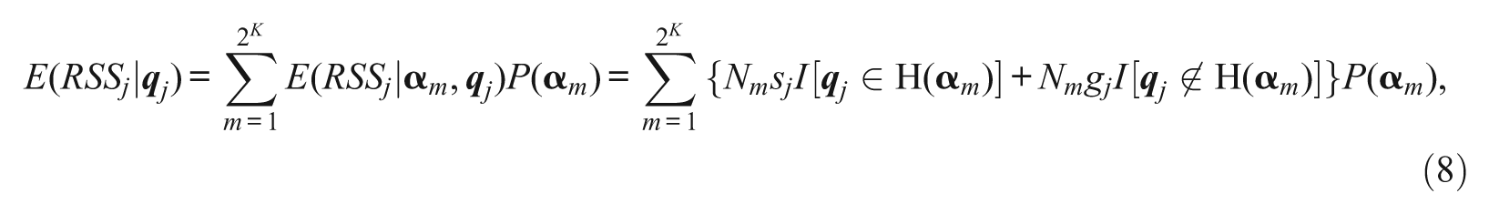
E (R S S_{j} | q_{j}) = \sum_{m = 1}^{2^{K}} E (R S S_{j} | α_{m}, q_{j}) P (α_{m}) = \sum_{m = 1}^{2^{K}} {N_{m} s_{j} I [q_{j} \in H (α_{m})] + N_{m} g_{j} I [q_{j} \notin H (α_{m})]} P (α_{m}),

where I[·] is the indicator function.

Let $q'_{j}$ represent a misspecified q-vector for item j. The next step is to determine $E (RS S_{j} | q'_{j})$ and compare it with $E (RS S_{j} | q_{j}) .$ Three cases must be distinguished:

Case 1: $q_{j}$ is nested within $q'_{j}$ .

Case 1 requires that Equations 7 and 8 be modified so that

E (R S S_{j} | α_{m}, q ’_{j}) = {\begin{matrix} N_{m} s_{j} \\ N_{m} (1 - g_{j}) \\ N_{m} g_{j} \end{matrix} \begin{matrix} if q_{j}, q ’_{j} \in H (α_{m}) \\ if q_{j} \in H (α_{m}), q ’_{j} \notin H (α_{m}) \\ otherwise \end{matrix},

and

E (R S S_{j} | q ’_{j}) = \sum_{m = 1}^{2^{K}} E (R S S_{j} | α_{m}, q ’_{j}) P (α_{m}) = \sum_{m = 1}^{2^{K}} {N_{m} s_{j} I [q_{j}, q ’_{j} \in H (α_{m})] + N_{m} (1 - g_{j}) I [q_{j} \in H (α_{m}), q ’_{j} \notin H (α_{m})] + N_{m} g_{j} I [q_{j} \notin H (α_{m})]} P (α_{m}),

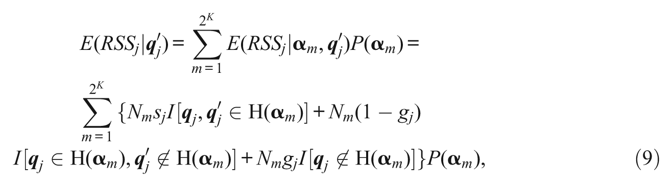
respectively. Comparing Equations 8 and 9 gives $E (RS S_{j} | q'_{j}) > E (RS S_{j} | q_{j})$ assuming that 1−g_j > s_j.

Case 2: $q'_{j}$ is nested within $q_{j} .$

The analogous modification of Equation 7 is

E (R S S_{j} | α_{m}, q ’_{j}) = {\begin{matrix} N_{m} s_{j} \\ N_{m} (1 - s_{j}) \\ N_{m} g_{j} \end{matrix} \begin{matrix} if q_{j}, q ’_{j} \in H (α_{m}) \\ if q ’_{j} \in H (α_{m}), q_{j} \notin H (α_{m}) \\ otherwise \end{matrix} .

The equivalent of Equation 9 is

E (R S S_{j} | q ’_{j}) = \sum_{m = 1}^{2^{K}} E (R S S_{j} | α_{m}, q ’_{j}) P (α_{m}) = \sum_{m = 1}^{2^{K}} {N_{m} s_{j} I [q_{j}, q ’_{j} \in H (α_{m})] + N_{m} (1 - s_{j}) I [q_{j} \in H (α_{m}), q ’_{j} \notin H (α_{m})] + N_{m} g_{j} I [q_{j} \notin H (α_{m})]} P (α_{m}) .

Therefore, assuming that 1−s_j > g_j, the same result $E (RS S_{j} | q'_{j}) > E (RS S_{j} | q_{j})$ is obtained for Case 2 as for Case 1.

Case 3: $q_{j}$ is not nested within $q'_{j}$ and $q'_{j}$ is not nested within $q_{j} .$

For this case, Equations 7 and 8 are modified to be

E (R S S_{j} | α_{m}, q ’_{j}) = {\begin{matrix} N_{m} s_{j} \\ N_{m} (1 - g_{j}) \\ N_{m} (1 - s_{j}) \\ N_{m} g_{j} \end{matrix} \begin{matrix} if q_{j}, q ’_{j} \in H (α_{m}) \\ if q_{j} \in H (α_{m}) and q ’_{j} \notin H (α_{m}) \\ if q ’_{j} \in H (α_{m}) and q_{j} \notin H (α_{m}) \\ otherwise \end{matrix} .

and

E (R S S_{j} | q ’_{j}) = \sum_{m = 1}^{2^{K}} E (R S S_{j} | α_{m}, q ’_{j}) P (α_{m}) = \sum_{m = 1}^{2^{K}} {N_{m} s_{j} I [q_{j}, q ’_{j} \in H (α_{m})] + N_{m} (1 - g_{j}) I [q_{j} \in H (α_{m}), q ’_{j} \notin H (α_{m})] + N_{m} (1 - s_{j}) I [q ’_{j} \in H (α_{m}), q_{j} \notin H (α_{m})] + N_{m} g_{j} I [q_{j} \notin H (α_{m}), q ’_{j} \notin H (α_{m})]} P (α_{m}),

respectively. Assuming that 1−s_j > g_j and 1−g_j > s_j, the same result $E (RS S_{j} | q'_{j}) > E (RS S_{j} | q_{j})$ is obtained for Case 3 as for Cases 1 and 2.

Note that the assumptions 1−g_j > s_j and 1−s_j > g_j are not additions to the existing assumptions of the DINA model, 1−g_j > g_j and 1−s_j > s_j. The assumptions of the DINA model imply that s_j and g_j are both less than 0.5, leading directly to 1−g_j > s_j and 1−s_j > g_j.

The derivations demonstrate that, if the examinees’ class memberships are known and s_j, g_j < 0.5, then the correct q-vector for each item is expected to be the q-vector with the lowest RSS among all possible q-vectors, provided that there is a sufficient number of examinees in each class. Theoretically, this is so regardless of the percentage of misspecified q-entries in the Q-matrix. In practice, however, the true class memberships are not known, and the interrelation of the misclassification of some examinees and a particular misspecified q-vector in the Q-matrix may decrease the RSS of the misspecified q-vector and increase the RSS of the correct q-vector. As a consequence, $E (RS S_{j} | q'_{j}) > E (RS S_{j} | q_{j})$ no longer holds, and the Q-matrix refinement method may not be able to identify the correct q-vector. This situation does not occur very often, and so it is reasonable to predict that it will not have much effect on the performance of the Q-matrix refinement method. The results of simulation studies examining the effectiveness and robustness of the method are presented later.

A noteworthy feature of the Q-matrix refinement method is that it is valid not only for observed item responses conforming to the DINA model but also for those conforming to any cognitive diagnosis model that incorporates the ideal item response η or any other ideal item response. To demonstrate the flexibility of the method, observed item responses conforming to the generalized NIDA model as well as those conforming to the DINA model are analyzed in the simulation studies.

It is important that the results of the Q-matrix refinement method applied to any data set collected for the evaluation of educational test performance be reviewed by experts in the domain of the test to resolve any ambiguities in those results. The method is best viewed as a supplement to, rather than as a replacement for, the judgments of experts in the educational domain.

Algorithm

The Q-matrix refinement method algorithm first identifies the q-vector that is most likely to be misspecified by finding the test item with the highest RSS. Although an item may have a high RSS due to random error rather than to misspecification, it is reasonable to assume that an item with a high RSS may be misspecified. For the targeted item, the algorithm searches over all 2^K− 1 possible q-vectors and replaces the q-vector under consideration with the q-vector with the lowest RSS. The algorithm continues until (a) all items have been visited and (b) the stopping criterion—that the RSS of each item no longer changes—has been met.

The steps of the algorithm are as follows:

Step 0: Initialize the search item pool as S⁽⁰⁾ = {1,…,J} and the input Q-matrix as Q ⁽⁰⁾.

Step 1: Use the nonparametric classification method (Chiu & Douglas, 2013) to estimate

examinees’ class memberships based on Q ⁽⁰⁾.

Step 2: Estimate the ideal item responses of all examinees based on Q ⁽⁰⁾ and the class

memberships estimated for them at Step 1.

Step 3: Compute the mean RSS across examinees for each observed response and its corresponding ideal response (estimated at Step 2) to each item. Select the item in S⁽⁰⁾ with the highest RSS. If the highest RSS occurs for item j, then denote the q-vector of the item as q _j⁽¹⁾, where the superscript (1) is the rank of the corresponding RSS among all items.

Step 4: Compute each remaining 2^K− 2 RSS by replacing q _j⁽¹⁾ in Q ⁽⁰⁾ with the other 2^K− 2 q-vectors, one at a time.

Step 5: Update Q ⁽⁰⁾ by replacing q _j⁽¹⁾ with q _j*⁽¹⁾, the q-vector with the lowest RSS among all the 2^K− 1 possible q-vectors. Call the updated Q-matrix as Q ⁽¹⁾.

Step 6: Omit item j out of the searching item pool. That is, S⁽¹⁾ = S⁽⁰⁾\{j}.

Step 7: Replace Q ⁽⁰⁾ and S⁽⁰⁾ with Q ⁽¹⁾ and S⁽¹⁾, respectively, and repeat Step 1 to Step 6. Iterate until all items have been visited.

Step 8: Repeat Step 1 to Step 7 until the RSS of each item no longer changes.

As indicated, the algorithm begins by targeting the item with the highest RSS and determining whether its q-vector should be updated. It may not be clear, however, whether a high RSS is due to a misspecified q-vector or to examinee misclassification, or is just inherently high (e.g., because of random error). If the RSS is inherently high, it can happen that the RSS for the item remains the highest even after that item has been evaluated, which will prevent the algorithm from continuing. To avoid revisiting an item with a high RSS but a correctly specified q-vector, the algorithm visits each item only once until all items have been evaluated. Because examinees are reclassified with every update of the Q-matrix, the RSS of each item decreases as the algorithm continues. Each update to the Q-matrix may provide new information that allows additional updates to the q-vectors, even those for items that have already been evaluated. Therefore, all items must usually be visited several times until the stopping criterion at Step 8 is met.

A remarkable feature of the Q-matrix refinement method algorithm is that it requires only a few iterations of (2^K− 1) ×J simple computations to refine and validate the Q-matrix input at Step 0. The algorithm described here is thus more efficient than other algorithms that have been proposed (e.g., Liu et al., 2012), even when the number of items and/or the number of attributes are large, at the cost of not necessarily finding a global optimum.

Simulation Studies

The performance of the Q-matrix refinement method is evaluated with three simulation studies that (a) explore its effectiveness, efficiency, and applicability; (b) determine the effects of the number of misspecified q-vectors and the number of misspecified q-entries on the recovery of the Q-matrix; and (c) ascertain the effect of the type of q-entry misspecification on the recovery of the correct Q-matrix, respectively.

Study 1: The Effectiveness, Efficiency, and Applicability of the Q-Matrix Refinement Method

The performance of existing Q-matrix validation methods (e.g., de la Torre, 2008; de la Torre & Chiu, 2010) has been evaluated only for Q-matrices with relatively small numbers of misspecified q-entries. For example, in de la Torre’s (2008) study, the maximum number of misspecified q-entries was 5 out of 150 (about 3.4%). To be useful, a Q-matrix validation or refinement method should be able to handle a much higher percentage of misspecified q-entries. Therefore, Study 1 was designed to evaluate the effectiveness, efficiency, and applicability of the Q-matrix refinement method with greater percentages of misspecified q-entries.

Design and Method

Seven variables were included in the study design: (a) number of examinees (N = 100, 500, 1,000), (b) number of test items (J = 20, 40, 80), (c) number of attributes (K = 3, 4, 5), (d) percentage of misspecified q-entries (10%, 20%), (e) source of the examinees’ attribute patterns (discrete uniform distribution, multivariate normal threshold model, higher-order model), (f) cognitive diagnosis model underlying the simulated item responses (DINA, NIDA), and (g) upper bound of the slipping and guessing parameters (0.2, 0.3, 0.4, 0.5).

The correct Q-matrices for tests containing 20 items and requiring possession of 3 or 4 attributes are shown in Table 1. When the number of attributes equals 5, there are more than 20 possible attribute patterns. Therefore, the correct Q-matrix for 5 attributes was constructed by including the 5 one-attribute patterns; 5, 5, and 4 randomly chosen two-, three-, and four-attribute patterns, respectively; and the single five-attribute pattern. An example of the Q-matrix used when the number of attributes equaled 5 is shown in Table 1. The Q-matrices for tests containing 40 and 80 items were constructed by doubling and quadrupling the 20-item Q-matrices, respectively. The correct Q-matrix was used to generate the simulated item responses; the misspecified Q-matrices were created by randomly changing either 10% or 20% of the q-entries in the correct Q-matrix from 0 to 1 or from 1 to 0. The misspecified Q-matrix was input to Step 0 of the Q-matrix refinement method algorithm.

Table 1.

Q-Matrices for Tests of 20 Items.

Number of attributes
3			4				5
1	0	0	1	0	0	0	1	0	0	0	0
0	1	0	0	1	0	0	0	1	0	0	0
0	0	1	0	0	1	0	0	0	1	0	0
1	1	0	0	0	0	1	0	0	0	1	0
1	0	1	1	0	0	0	0	0	0	0	1
0	1	1	0	1	0	0	1	1	0	0	0
1	0	0	0	0	1	0	0	1	0	1	0
0	1	0	0	0	0	1	1	0	0	0	1
0	0	1	1	1	0	0	0	0	0	1	1
1	1	0	1	0	1	0	0	0	1	1	0
1	0	1	1	0	0	1	0	1	1	1	0
0	1	1	0	1	1	0	1	0	1	0	1
1	0	0	0	1	0	1	0	1	0	1	1
0	1	0	0	0	1	1	0	0	1	1	1
0	0	1	1	1	1	0	1	1	1	0	0
1	1	0	1	1	0	1	1	1	1	0	1
1	0	1	1	0	1	1	0	1	1	1	1
0	1	1	0	1	1	1	1	1	0	1	1
1	1	1	1	1	1	1	1	0	1	1	1
1	1	1	1	1	1	1	1	1	1	1	1

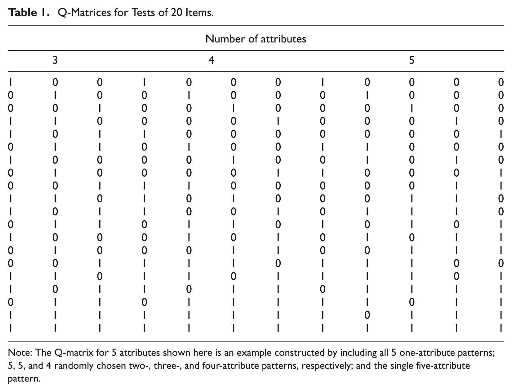
Note: The Q-matrix for 5 attributes shown here is an example constructed by including all 5 one-attribute patterns; 5, 5, and 4 randomly chosen two-, three-, and four-attribute patterns, respectively; and the single five-attribute pattern.

The source of the examinees’ attribute patterns was the discrete uniform distribution with equal probabilities, the multivariate normal threshold model (Chiu et al., 2009), or the higher-order model (de la Torre & Douglas, 2004). The multivariate normal threshold model represents a realistic situation in which attributes are correlated rather than independent, and attribute patterns do not have equal probabilities of occurrence. It was assumed that a multivariate normal distribution underlay the discrete attribute patterns, which were drawn from a multivariate normal distribution MVN(0_K, Σ), with all variances and covariances in the variance-covariance matrix equal to 1.0 and 0.5, respectively. Let the underlying continuous ability for examinee i be θ_i = (θ_i1,…,θ_iK). The attribute pattern α_i = (α_i1,…,α_iK) was determined by

α_{i k} = {\begin{matrix} 1 if θ_{i k} \geq Φ^{- 1} (\frac{k}{K + 1}) \\ 0 otherwise \end{matrix}

where k = 1,…,K.

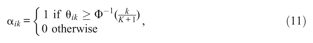
The higher-order model assumed that the entries in the attribute pattern for examinee i were associated with a general unidimensional latent ability, δ_i, through a logit link. That is, the probability of possessing the attribute k, α_ik, was

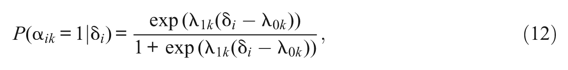
P (α_{ik} = 1 | δ_{i}) = \frac{\exp (λ_{1 k} {(δ}_{i} - λ_{0 k}))}{1 + \exp (λ_{1 k} (δ_{i} - λ_{0 k}))}

where λ_0k and λ_1k are structural parameters, and λ_1k > 0. The K attributes were assumed to be conditionally independent given δ_i; therefore, the joint probability of the attribute patterns was

P (α_{i} | δ_{i}) = \prod_{k = 1}^{K} P (α_{i k} {|δ}_{i}) .

In this simulation, δ_i was drawn from N(0, 1); λ_0k and λ_1k were drawn from N(0, 1) and logN(0, 0.5), respectively.

Examinees’ simulated item responses were generated to conform either to the DINA model or to the NIDA model, with the upper bound of the slipping and guessing parameters set to 0.2, 0.3, 0.4, or 0.5.

Twenty-five data sets were generated for each of the 3 (examinee) × 3 (item) × 3 (attribute) × 2 (misspecification) × 3 (source) × 2 (model) × 3 (slipping/guessing) = 972 conditions in the design. Each data set was analyzed using the Q-matrix refinement method algorithm with a misspecified Q-matrix input to Step 0. Two statistics—CPU time and q-entry recovery rate—were computed for each data set and then averaged across the 25 data sets in each design condition. The q-entry recovery rate equals the ratio of the number of correct q-entries in the final refined Q-matrix to the total number of q-entries. The accuracy base rates were 0.90 and 0.80 for design conditions with 10% and 20% misspecification, respectively. A q-entry recovery rate close to the base rate is less informative; a q-entry recovery rate greater than the base rate is more informative.

Results

Because the impacts of the various factors on the mean q-entry recovery rates (MRRs) for tests of different lengths (i.e., J = 20, 40, and 80) were the same and the MRRs for tests of 40 and 80 items were higher than those of 20 items, only the results for tests of 20 items are included in the tables.

Table 2 presents the mean recovery rates of the correct q-entries from the misspecified q-entries for simulated item responses conforming to the DINA model and J = 20. When the source of the attribute patterns was the discrete uniform distribution, the MRRs indicated perfect or near perfect recovery when the upper bound of the slipping and guessing parameters was less than or equal to 0.4 and the number of attributes equaled 3 or 4; they were a bit lower but still very high when the number of attributes equaled 5. Although an upper bound of the slipping and guessing parameters equal to 0.5 is the maximum accepted by the Q-matrix refinement algorithm, the MRRs for this value of the upper bound were reasonably high. The MRRs when the source of the attribute patterns was either the multivariate normal threshold model or the higher order model were lower than those when the source was the discrete uniform distribution, with those when the source was the multivariate normal threshold model slightly higher than those when the source was the higher order model.

Table 2.

Mean Q-Entries Recovery Rate: DINA Model, 20 Items.

		Source of attribute patterns
		Discrete uniform			Multivariate normal threshold			Higher order
		N			N			N
K	Maximum s	100	500	1,000	100	500	1,000	100	500	1,000
10% Q-matrix misspecification
3	0.2	1.00	1.00	1.00	0.96	0.99	0.99	0.97	0.99	1.00
	0.3	0.99	1.00	1.00	0.95	0.98	0.98	0.98	0.99	0.99
	0.4	0.97	1.00	1.00	0.90	0.95	0.97	0.93	0.98	0.98
	0.5	0.90	0.95	0.96	0.86	0.92	0.93	0.86	0.93	0.94
4	0.2	0.98	1.00	1.00	0.91	0.96	0.97	0.95	0.98	0.97
	0.3	0.97	1.00	1.00	0.89	0.95	0.95	0.93	0.98	0.99
	0.4	0.94	0.98	0.98	0.88	0.92	0.93	0.89	0.97	0.96
	0.5	0.89	0.92	0.94	0.84	0.89	0.91	0.87	0.91	0.91
5	0.2	0.95	0.99	0.99	0.87	0.91	0.92	0.9	0.95	0.97
	0.3	0.93	0.96	0.97	0.85	0.90	0.92	0.87	0.93	0.95
	0.4	0.87	0.93	0.93	0.82	0.89	0.91	0.87	0.91	0.91
	0.5	0.85	0.89	0.91	0.82	0.86	0.88	0.82	0.88	0.92
20% Q-matrix misspecification
3	0.2	1.00	1.00	1.00	0.94	0.95	0.96	0.97	0.99	0.97
	0.3	0.98	1.00	1.00	0.91	0.92	0.95	0.89	0.98	0.99
	0.4	0.95	0.99	1.00	0.87	0.90	0.91	0.89	0.96	0.97
	0.5	0.88	0.92	0.93	0.80	0.86	0.86	0.84	0.90	0.90
4	0.2	0.93	0.99	0.98	0.83	0.87	0.92	0.91	0.97	0.95
	0.3	0.93	0.97	0.98	0.83	0.87	0.87	0.89	0.92	0.95
	0.4	0.87	0.91	0.91	0.81	0.83	0.87	0.83	0.89	0.89
	0.5	0.79	0.85	0.86	0.75	0.81	0.80	0.79	0.83	0.85
5	0.2	0.86	0.88	0.93	0.79	0.83	0.81	0.84	0.90	0.88
	0.3	0.82	0.86	0.88	0.79	0.82	0.82	0.80	0.85	0.86
	0.4	0.80	0.83	0.83	0.74	0.81	0.82	0.78	0.83	0.85
	0.5	0.74	0.81	0.81	0.73	0.79	0.80	0.76	0.80	0.81

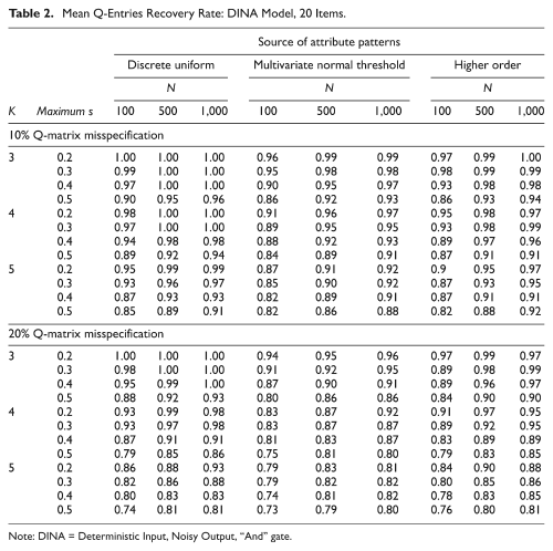
Note: DINA = Deterministic Input, Noisy Output, “And” gate.

It is not surprising that the MRRs increased as the number of examinees increased, but a large number of examinees was not necessary for a high MRR when the source of the attribute patterns was the discrete uniform distribution; N = 100 was sufficient to ensure excellent recovery. It is surprising that the MRRs increased as the number of items increased. One might expect that recovery would be more difficult for a long test, because, given a particular misspecification percentage, the number of misspecified q-entries increases as the number of items increases. However, the nonparametric classification method embedded in the Q-matrix refinement method is known to yield higher classification rates for longer tests (Chiu & Douglas, 2013), which in turn appeared to boost the q-entry recovery rate for long tests.

The differences in the MRRs across the three sources of attribute patterns were greater for 20% misspecification than for 10% misspecification; the smaller the number of examinees, the greater the differences. It may be that, when the source of the attribute patterns was the multivariate normal threshold model or the higher-order model, some classes contained few or even no examinees, especially when the number of attributes was large. In this situation, the RSS might have provided limited or biased information, which then resulted in poor recovery. For example, if the q-vector (110) was misspecified as (100), the misspecified q-entry could be detected only if there were sufficient examinees with attribute patterns of (100) or (101) because the item responses of the examinees in the other classes did not provide useful diagnostic information about the item.

Table 3 presents the mean recovery rates of the correct q-entries from the misspecified q-entries for item responses conforming to the NIDA model and J = 20. The performance of the Q-matrix refinement method was excellent when the source of the attribute patterns was the discrete uniform distribution and still very good when the source was the higher order model. Differences in the MRRs when the sources of the attribute patterns were the higher order model and the multivariate normal threshold model were noticeable only when the number of examinees was small and the number of attributes was large, suggesting that the performance of the Q-matrix refinement method was not much influenced by the source of the attribute patterns as long as there were sufficient examinees in each class. As was the case in Table 2, the MRRs decreased as the number of attributes or the upper bound of the slipping and guessing parameters increased.

Table 3.

Mean Q-Entry Recovery Rate: NIDA Model, 20 Items.

		Source of attribute patterns
		Discrete uniform			Multivariate normal threshold			Higher order
		N			N			N
K	Maximum s	100	500	1,000	100	500	1,000	100	500	1,000
10% Q-matrix misspecification
3	0.2	1.00	1.00	1.00	0.94	0.99	0.99	0.98	1.00	1.00
	0.3	0.99	1.00	1.00	0.92	0.97	0.98	0.93	1.00	1.00
	0.4	0.95	0.99	0.99	0.89	0.94	0.95	0.88	0.95	0.98
	0.5	0.91	0.95	0.95	0.85	0.92	0.92	0.93	0.92	0.93
4	0.2	0.98	0.99	1.00	0.90	0.96	0.95	0.97	0.99	0.98
	0.3	0.95	0.98	0.98	0.88	0.94	0.94	0.95	0.98	0.98
	0.4	0.91	0.95	0.95	0.85	0.93	0.92	0.86	0.94	0.95
	0.5	0.87	0.92	0.92	0.84	0.89	0.91	0.90	0.89	0.90
5	0.2	0.92	0.95	0.97	0.85	0.90	0.92	0.92	0.98	0.98
	0.3	0.90	0.93	0.94	0.84	0.89	0.90	0.92	0.89	0.94
	0.4	0.88	0.90	0.92	0.84	0.88	0.90	0.88	0.91	0.91
	0.5	0.83	0.90	0.90	0.82	0.87	0.88	0.78	0.87	0.90
20% Q-matrix misspecification
3	0.2	0.98	1.00	1.00	0.93	0.95	0.92	0.95	0.99	0.98
	0.3	0.98	0.99	1.00	0.89	0.94	0.95	0.92	0.96	0.97
	0.4	0.90	0.96	0.97	0.81	0.86	0.89	0.84	0.90	0.94
	0.5	0.84	0.86	0.87	0.80	0.82	0.84	0.83	0.87	0.87
4	0.2	0.93	0.95	0.97	0.81	0.87	0.90	0.90	0.96	0.94
	0.3	0.87	0.93	0.93	0.80	0.85	0.86	0.86	0.90	0.89
	0.4	0.80	0.88	0.86	0.76	0.81	0.83	0.81	0.85	0.87
	0.5	0.79	0.83	0.83	0.77	0.80	0.81	0.80	0.82	0.85
5	0.2	0.81	0.88	0.86	0.74	0.80	0.81	0.80	0.88	0.86
	0.3	0.77	0.83	0.84	0.76	0.81	0.82	0.78	0.83	0.84
	0.4	0.76	0.80	0.81	0.74	0.79	0.80	0.78	0.81	0.81
	0.5	0.74	0.79	0.79	0.72	0.78	0.79	0.73	0.79	0.80

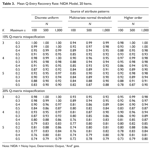
Note: NIDA = Noisy Input, Deterministic Output, “And” gate.

Table 3 also shows that the performance of the Q-matrix refinement method was excellent when the source of the attribute patterns was either the discrete uniform distribution or the higher order model, but deteriorated slightly when the source was the multivariate normal threshold model. The ratios of the correct q-entries recovered from the misspecified q-entries for the two misspecification percentages indicated that misspecification percentage had little or no impact on the effectiveness of the Q-matrix refinement method.

Comparison of the MRRs for item responses conforming to the DINA model with those for item responses conforming to the NIDA model suggest that the Q-matrix refinement method was generally less tolerant of larger values of the upper bound of the slipping and guessing parameters for item responses generated from the NIDA model, with slight decreases in the MRRs when the number of attributes was large. It may not be appropriate, however, to ascribe this intolerance to the fact that a method developed for item responses conforming to the DINA model was applied to item responses conforming to the NIDA model, because in the NIDA model, slipping and guessing operates at the attribute level, not at the item level, and so their effects can be multiplicative. Therefore, a comparative evaluation of the performance of the Q-matrix refinement method across the two models may not be valid.

The Q-matrix refinement method algorithm, which was implemented in the software environment R, was very efficient, using little computer time. On average, it took the algorithm only 1 s (for N = 100, J = 20, K = 3, maximum s (max.s) = 0.2) to 10 min (for N = 1,000, J = 80, K = 5, max.s = 0.5) to complete an analysis. The misspecification percentage had little effect on efficiency.

Study 2: Effects of the Number of Misspecified Q-Vectors and the Number of Misspecified Q-Entries on Q-Matrix Recovery

The comparison in Study 1 between the MRRs for Q-matrices with 10% misspecification and Q-matrices with 20% misspecification did not clarify the relation between the percentage of misspecification and the MRR. Therefore, Study 2 was designed to determine the effects of the number of misspecified q-vectors (N_mis.v) and the number of misspecified q-entries (N_mis.e) on Q-matrix recovery.

Design and Method

The Q-matrix with J = 80 items and K = 4 attributes from Study 1 was used as the correct Q-matrix. The number of examinees was set to 1,000. To avoid confounding, either the N_mis.v or N_mis.e was controlled while the other was varied. N_mis.v was varied from 10 to 40. N_mis.e was varied from 1 to 40, with only one misspecified q-entry appearing in any one q-vector. (N_mis.e equal to 40 is equivalent to 12.5% misspecified q-entries in the Q-matrix.) Each misspecified Q-matrix was created by randomly changing the appropriate number of q-entries from 0 to 1 or from 1 to 0, and then input to Step 0 of the Q-matrix refinement method algorithm. Simulated item responses were generated from the DINA model with the source of the attribute patterns being either the discrete uniform distribution or the higher order model. The upper bound of the slipping and guessing parameters took on the values 0.2, 0.3, and 0.4. Twenty-five data sets were generated for each condition of the design.

N_mis.v was plotted against the MRR computed across the 25 data sets for each design condition. Because different values of N_mis.e correspond to different accuracy base rates, however, a particular value of the MRR reflects a different degree of recovery success for different values of N_mis.e. For example, for a Q-matrix with 20 items, 5 attributes, and N_mis.e = 1, the base rate accuracy equals 0.99. Therefore, a MRR of 0.99 indicates that the Q-matrix refinement method was not successful in recovering the correct q-entry for the single misspecified q-entry. If N_mis.e = 20 for the same Q-matrix, the base rate accuracy equals 0.80. Then, a MRR of 0.99 indicates that the Q-matrix refinement method was able to recover the correct q-entry for 19 of the 20 misspecified q-entries, a much greater degree of success. Therefore, N_mis.e was plotted against the mean number of recovered q-entries computed across the 25 data sets for each design condition rather than against the MRR.

Results

The results of the simulation for all design conditions for which the source of the attribute patterns was the discrete uniform distribution were not sufficiently distant from perfect recovery to be able to discern any effect of N_mis.v or N_mis.e on q-entry recovery. In addition, the results for different max.s levels appeared to follow the same pattern. Therefore, only the results for design conditions in which the source of the attribute patterns was the higher-order model and max.s = 0.4 (i.e., the most extreme case) are displayed in the figure.

Figure 1a shows the relation between N_mis.v and the MRR for max.s = 0.4. The horizontal dashed reference line in the figure represents the mean of the MRRs. Examination of Figure 1a shows that the points representing the MRRs are scattered randomly around and close to the reference line, implying that, given that the number of misspecified q-entries was fixed, the performance of the Q-matrix refinement method was not affected by the number of misspecified q-vectors.

Figure 1.

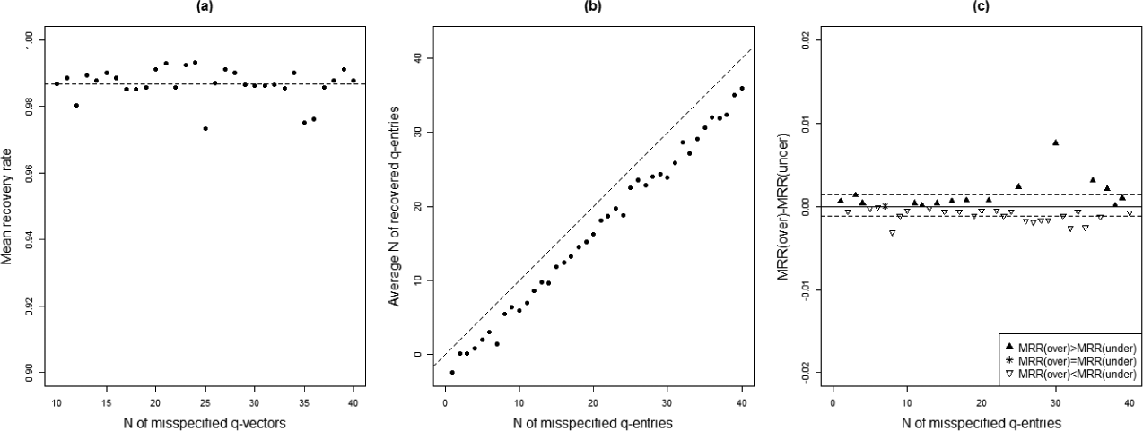
(a) Number of misspecified q-vectors (N_mis.v) plotted against MRR, (b) number of misspecified q-entries (N_mis.e) plotted against mean number of recovered q-entries, (c) number of misspecified q-entries (N_mis.e) plotted against difference in MRR for paired analyses using overspecified and underspecified Q-matrix as input to the Q-matrix refinement method algorithm.

Figure 1b shows the relation between N_mis.e and the mean number of recovered q-entries for max.s = 0.4. The diagonal dashed reference line Y = X in the figure represents perfect q-entry recovery. Examination of Figure 1b shows that the points representing the mean number of recovered q-entries all lie below and close to the reference line in no discernible pattern, although there is a slight tendency for points representing low values of N_mis.e (i.e., 1-10) to lie closer to the reference line than points representing high values of N_mis.e (i.e., 30-40). It appears, therefore, that the number of misspecified q-entries had little effect on the performance of the Q-matrix refinement method.

Study 3: Effect of Misspecification Type on Q-Matrix Recovery

There are two types of misspecification in a binary Q-matrix: overspecification, when q-entries of 0 are incorrectly coded as 1, and underspecification, when q-entries of 1 are incorrectly coded as 0. The simulation studies presented thus far changed correct q-entries to misspecified q-entries randomly and did not distinguish between overspecification and underspecification. Knowing whether the Q-matrix refinement method handles the two types of misspecification differently may aid in the interpretation of the results obtained from the Q-matrix refinement method. Therefore, Study 3 was designed to determine whether the effectiveness of the method is affected by the type of misspecification.

Design and Method

The number of examinees, the number of items, and the number of attributes were fixed at 1,000, 80, and 4, respectively; N_mis.e ranged from 1 to 40; and the upper bound of the slipping and guessing parameters took on the values 0.2, 0.3, and 0.4. Twenty-five data sets were generated for each condition of the design. Simulated item responses were generated from the DINA model with the source of the attribute patterns being the higher order model.

Each data set was analyzed twice, once using a purely overspecified Q-matrix and once using a purely underspecified Q-matrix as input to Step 0 of the Q-matrix refinement method algorithm. As in Study 2, each misspecified q-vector contained only one misspecified q-entry to avoid confounding N_mis.e with N_mis.v, although it was shown that N_mis.v does not affect Q-matrix recovery.

For each set of paired analyses, the MRR (across the 25 data sets) computed for the analysis using the underspecified Q-matrix was subtracted from the MRR computed for the analysis using the overspecified Q-matrix; these differences were then plotted against the number of misspecified q-entries. The distance from each difference point to the horizontal solid reference line Y = 0 equals the difference between the two MRRs.

Results

Each solid triangle, open triangle, and asterisk in Figure 1c represents a value of N_mis.e for which the difference between the two MRRs for the paired analyses was positive, negative, or zero, respectively. The means of these differences for the positive-difference cases and the negative-difference cases are represented by horizontal dashed lines above and below the reference line, on which the zero-difference cases fall.

A glance at Figure 1c suggests that the Q-matrix refinement method was as successful in Q-matrix recovery for the analyses based on the underspecified Q-matrix as it was for the analyses based on the overspecified Q-matrix when N_mis.e was less than 25, but was less successful when N_mis.e was greater than 25. Note, though, that all differences between the MRRs lie between −0.01 and 0.01, a range too narrow to conclude that the type of Q-matrix misspecification had any effect on Q-matrix recovery.

Real Data Analysis

The Fraction-Subtraction Data Set

In addition to being applied to simulated data, the Q-matrix refinement method was applied to a real data set, Tatsuoka’s (1984) well-known fraction-subtraction data. This data set consists of the binary responses of 536 middle-school students to 20 arithmetic problems requiring the subtraction of fractions; these problems are listed in Table 4, which also provides the Q-matrix and describes the skills (attributes) needed to respond correctly to the problems.

Table 4.

Problems and Q-Matrix for the Fraction-Subtraction Data (Tatsuoka, 1984).

		Q-Matrix
Item	Problem	S1	S2	S3	S4	S5	S6	S7	S8
1	$\frac{5}{3} - \frac{3}{4}$	0	0	0	1	0	1	1	0
2	$\frac{3}{4} - \frac{3}{8}$	0	0	0	1	0	0	1	0
3	$\frac{5}{6} - \frac{1}{9}$	0	0	0	1	0	0	1	0
4	$3 \frac{1}{2} - 2 \frac{3}{2}$	0	1	1	0	1	0	1	0
5	$4 \frac{3}{5} - 3 \frac{4}{10}$	0	1	0	1	0	0	1	1
6	$\frac{6}{7} - \frac{4}{7}$	0	0	0	0	0	0	1	0
7	$3 - 2 \frac{1}{5}$	1	1	0	0	0	0	1	0
8	$\frac{2}{3} - \frac{2}{3}$	0	0	0	0	0	0	1	0
9	$3 \frac{7}{8} - 2$	0	1	0	0	0	0	0	0
10	$4 \frac{4}{12} - 2 \frac{7}{12}$	0	1	0	0	1	0	1	1
11	$4 \frac{1}{3} - 2 \frac{4}{3}$	0	1	0	0	1	0	1	0
12	$1 \frac{1}{8} - \frac{1}{8}$	0	0	0	0	0	0	1	1
13	$3 \frac{3}{8} - 2 \frac{5}{6}$	0	1	0	1	1	0	1	0
14	$3 \frac{4}{5} - 3 \frac{2}{5}$	0	1	0	0	0	0	1	0
15	$2 - \frac{1}{3}$	1	0	0	0	0	0	1	0
16	$4 \frac{5}{7} - 1 \frac{4}{7}$	0	1	0	0	0	0	1	0
17	$7 \frac{3}{5} - \frac{4}{5}$	0	1	0	0	1	0	1	0
18	$4 \frac{1}{10} - 2 \frac{8}{10}$	0	1	0	0	1	1	1	0
19	$4 - 1 \frac{4}{3}$	1	1	1	0	1	0	1	0
20	$4 \frac{1}{3} - 1 \frac{5}{3}$	0	1	1	0	1	0	1	0

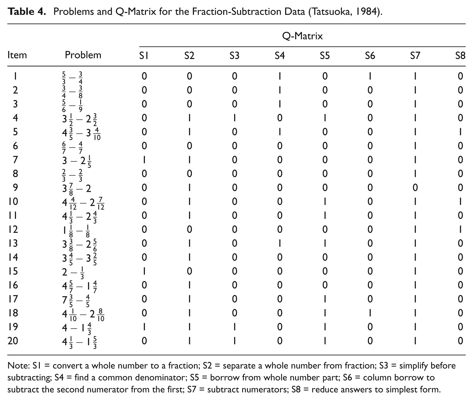
Note: S1 = convert a whole number to a fraction; S2 = separate a whole number from fraction; S3 = simplify before subtracting; S4 = find a common denominator; S5 = borrow from whole number part; S6 = column borrow to subtract the second numerator from the first; S7 = subtract numerators; S8 = reduce answers to simplest form.

DeCarlo (2011) fitted several extended DINA models to the fraction-subtraction data and noted that large estimates of class sizes might indicate that the Q-matrix has been misspecified. He suggested that possession of the third skill (S3: simplify before subtracting) was not required to respond correctly to any of the items and that S3 should be eliminated from the Q-matrix.

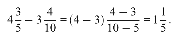
Unfortunately, the Q-matrix for the fraction-subtraction data is not complete. A complete Q-matrix allows identification of all possible attribute patterns and requires that each attribute be represented by at least one single-attribute item (for proof, see Chiu et al., 2009). Therefore, it may not be possible to identify the attribute patterns of all 536 examinees. Inspection of the ideal item response patterns indicated that only 58 of the 2⁸ = 256 possible attribute patterns can be identified by the items, an indication that multiple classes may be collapsed. For example, 64 of the 256 attribute patterns correspond to the ideal item response pattern consisting of all zeroes. In this situation, the assignment of an examinee whose attribute pattern cannot be identified to a class is a random process that may result in misclassification. Accordingly, the Q-matrix refinement method algorithm was run multiple times, producing two different results. In partial agreement with DeCarlo (2011), the first result indicated that possession of the third attribute was not required to respond correctly to Item 4. The second result concurred with the first and also indicated that possession of the seventh skill (S7: subtract numerators) was not required to respond correctly to Item 5. Note that an incorrect strategy for solving the problem ( $4 \frac{3}{5} - 3 \frac{4}{10}$ ) in Item 5—subtract the first numerator from the second numerator and subtract the first denominator from the second denominator—happens to give the correct answer:

4 \frac{3}{5} - 3 \frac{4}{10} = (4 - 3) \frac{4 - 3}{10 - 5} = 1 \frac{1}{5} .

This example serves as a reminder that input from experts in the educational domain of the test is essential to the correct interpretation of the results produced by the Q-matrix refinement method.

Simulation Study Based on Model Parameters

A simulation study was conducted to verify that the Q-matrix refinement method can be effectively applied to the fraction-subtraction data. De la Torre and Douglas (2004) used a Markov chain Monte Carlo (MCMC) algorithm to fit a higher order DINA model to the fraction-subtraction data, with good results. Therefore, the model parameter estimates from their study (see Tables 11 and 12 on pp. 350-351, de la Torre and Douglas, 2004) were used to generate 25 data sets, each with 536 examinees and 20 items requiring possession of up to eighty skills for a correct response. The Q-matrix shown in Table 4 was assumed to be the correct Q-matrix and used to generate the simulated item responses. Because the number of misspecified q-entries is unknown in practice, and because, as demonstrated by the earlier simulation studies, the misspecification percentage has little effect on the performance of the Q-matrix refinement method, it was decided to construct a Q-matrix with 10% misspecification by randomly altering 16 (20 items × 8 attributes × 0.10) q-entries in the Q-matrix from 0 to 1 or from 1 to 0. The misspecified Q-matrix was input to Step 0 of the Q-matrix refinement method algorithm.

As mentioned earlier, a test requiring possession of eight skills but containing only 20 items is too short to identify all 256 possible attribute patterns. Therefore, it was to be expected that the Q-matrix refinement method would be hampered in its ability to recover the correct q-entries from the misspecified q-entries. The result shows that the method recovered on average 4.6 correct q-entries from the 16 misspecified q-entries (28.75%), which might be taken as an indication that the performance of the method can be affected in situations where short tests are used to measure a relatively large number of skills.

Discussion

Validating the Q-matrix for a given test is a serious problem in cognitive diagnosis research. Various solutions to this problem have been proposed (e.g., Barnes, 2010; de la Torre, 2008; de la Torre & Chiu, 2010; Liu et al., 2012), but computational feasibility, the identification of misspecified q-entries, and the difficulty of distinguishing between a misspecified Q-matrix and a genuinely ill-fitting cognitive diagnosis model remain problematic. The Q-matrix refinement method described in this article offers an alternative solution. The three simulation studies using this method and the application to a real data set demonstrated that it is both effective and efficient in recovering the correct Q-matrix from a misspecified Q-matrix under a variety of conditions. The numbers of misspecified q-entries and q-vectors, and the type of misspecification have little effect on the performance of the method, enhancing its applicability. Moreover, for observed item responses conforming to the DINA model or to the generalized NIDA model, the method tolerates a substantial degree of error perturbation of those responses. However, it should be noted that the Q-matrix refinement method may be limited in dealing with other types of misspecifications in the Q-matrix, such as the misspecification of the total number of attributes. The method can be used to delete a redundant skill from the Q-matrix, but it cannot detect skills that have been entirely missed. Similarly, the Q-matrix refinement method cannot identify a misspecified cognitive diagnosis model, but the method can be used as a logical first step in addressing misfit concerns. After the Q-matrix has been cleaned up, any remaining indication of misfit can be very likely attributed to the misspecification of the cognitive diagnosis model supposed to underlie the data.

The simulation studies raise the question of why the q-entry recovery rates were not as good when the source of the examinees’ attribute patterns was the realistic multivariate normal threshold model rather than the discrete uniform distribution. The reason may be that some proficiency classes may have contained too few examinees to be able to identify a misspecified q-vector for an item by minimizing that item’s RSS. An obvious solution to this problem is to develop a loss function that is independent of the class size. Consider Equation 9. (Developing loss functions for Equations 8 and 10 follows the same principle.) A rescaled loss function, $E [RS S_{j} | q_{j}'] / N_{m}$ , can be directly established by

\frac{E [R S S_{j} | q_{j}^{’}]}{N_{m}} = \sum_{m = 1}^{2^{K}} {s_{j} I [q_{j}, q_{j}^{’} \in H (α_{m})] + (1 - g_{j}) I [q_{j} \in H (α_{m}), q_{j}^{’} \notin H (α_{m})] + g_{j} I [q_{j} \notin H (α_{m})]} P (α_{m}) .

The rescaled loss function preserves the relation $E [R S S_{j} | q_{j}^{’}] / N_{m} > E [R S S_{j} | q_{j}] / N_{m}$ ; the right-hand side of Equation 13 indicates that it does not rely on the class size N_m. So, this loss function should be more appropriate for a data set with proficiency classes containing only a few examinees. A preliminary simulation study indicates that the Q-matrix refinement method algorithm using the rescaled loss function does indeed improve the q-entry recovery rate; however, with the currently implemented stopping criterion, the method consumes much more computer time than does the algorithm using the original loss function. Taking into consideration both the improvement in the q-entry recovery rate and the increase in computer time for the algorithm using the rescaled loss function, the algorithm using the original loss function seems preferable. Future research could focus on identifying a better stopping criterion for the algorithm using the rescaled loss function.

Other research might focus on improving the rate of detection of the misspecified q-entries and q-vectors. For example, the RSS used as a test criterion for each item could be differentially weighted to reflect individual variation in the observed item responses.

The fact that the Q-matrix refinement method is nonparametric is advantageous because no commitment to a possibly questionable parameter structure supposed to determine educational test performance is required. Additional advantages of the method include the fact that, unlike the parametric model based approaches to Q-matrix validation, it requires neither a large number of examinees nor a great deal of computer time. Thus, the method should be of particular benefit to small and medium-sized educational testing programs.

Footnotes

Declaration of Conflicting Interests

The author(s) declared no potential conflicts of interest with respect to the research, authorship, and/or publication of this article.

Funding

The author(s) received no financial support for the research, authorship, and/or publication of this article.

References

Ayers

Nugent

Dean

(2008). Skill set profile clustering based on student capability vectors computed from online tutoring data. In de Baker

R. S. J.

Barnes

Beck

J. E.

(Eds.), Educational data mining: Proceedings of the 1st international conference on education data mining (pp. 210-217). Montréal, Québec, Canada: International Data Mining Society.

Barnes

(2010). Novel derivation and application of skill matrices: The q-matrix method. In Ramero

Vemtora

Pechemizkiy

de Baker

R. S. J.

(Eds.), Handbook of educational data mining (pp. 159-172). Boca Raton, FL: Chapman & Hall.

Chiu

C.-Y.

Douglas

J. A.

(2013). A nonparametric approach to cognitive diagnosis by proximity to ideal item response patterns. Journal of Classification, 30, 225-250.

Chiu

C.-Y.

Douglas

(2009). Cluster analysis for cognitive diagnosis: Theory and applications. Psychometrika, 74, 633-665.

Chiu

C.-Y.

Seo

(2009). Cluster analysis for cognitive diagnosis: An application to the 2001 PIRLS reading assessment. IERI Monograph Series, 2, 137-159.

DeCarlo

L. T.

(2011). On the analysis of fraction subtraction data: The DINA model, classification, latent class sizes, and the Q-matrix. Applied Psychological Measurement, 35, 8-26.

DeCarlo

L. T.

(2012). Recognizing uncertainty in the Q-matrix via a Bayesian extension of the DINA model. Applied Psychological Measurement, 36, 447-468.

de la Torre

(2008). An empirically based method of Q-matrix validation for the DINA model: Development and applications. Journal of Educational Measurement, 45, 343-362.

de la Torre

(2009). DINA model and parameter estimation: A didactic. Journal of Educational and Behavioral Statistics, 34, 115-130.

10.

de la Torre

(2011). The generalized DINA model framework. Psychometrika, 76, 179-199.

11.

de la Torre

Chiu

C.-Y.

(2010, April). A general empirical method of Q-matrix validation. Paper presented at the annual meeting of the National Council on Measurement in Education, Denver, CO.

12.

de la Torre

Douglas

J. A.

(2004). Higher-order latent trait models for cognitive diagnosis. Psychometrika, 69, 333-353.

13.

de la Torre

Douglas

J. A.

(2008). Model evaluation and multiple strategies in cognitive diagnosis: An analysis of fraction subtraction data. Psychometrika, 73, 595-624.

14.

Haertel

E. H.

(1989). Using restricted latent class models to map the skill structure of achievement items. Journal of Educational Measurement, 26, 301-321.

15.

Hartz

S. M.

Roussos

L. A.

Henson

R. A.

Templin

J. L.

(2005). The fusion model for skill diagnosis: Blending theory with practicality. Unpublished manuscript.

16.

Henson

R. A.

Templin

J. L.

Willse

J. T.

(2009). Defining a family of cognitive diagnosis models using log-linear models with latent variables. Psychometrika, 74, 191-210.

17.

Junker

B. W.

Sijtsma

(2001). Cognitive assessment models with few assumptions, and connections with nonparametric item response theory. Applied Psychological Measurement, 25, 258-272.

18.

Liu

Ying

(2012). Data-driven learning of Q-matrix. Applied Psychological Measurement, 36, 609-618.

19.

Macready

G. B.

Dayton

C. M.

(1977). The use of probabilistic models in the assessment of mastery. Journal of Educational and Behavioral Statistics, 2, 99-120.

20.

Maris

(1999). Estimating multiple classification latent class models. Psychometrika, 64, 187-212.

21.

Rupp

A. A.

Templin

(2008). The effects of Q-matrix misspecification on parameter estimates and classification accuracy in the DINA model. Educational and Psychological Measurement, 68, 78-96.

22.

Tatsuoka

K. K.

(1984). Analysis of errors in fraction addition and subtraction problems (Report No. NIE-G-81–0002). Urbana: Computer-based Education Research Laboratory, University of Illinois.

23.

Tatsuoka

K. K.

(1985). A probabilistic model for diagnosing misconceptions by the pattern classification approach. Journal of Educational and Behavioral Statistics, 10, 55-73.

24.

Tatsuoka

K. K.

(1990). Toward an integration of item-response theory and cognitive error diagnosis. In Frederiksen

Glaser

Lesgold

Shafto

(Eds.), Diagnostic monitoring of skill and knowledge acquisition (pp. 453-488). Hillsdale, NJ: Erlbaum.

25.

Tatsuoka

K. K.

Tatsuoka

M. M.

(1987). Bug distribution and pattern classification. Psychometrika, 52, 193-206.

26.

Tatsuoka

K. K.

Tatsuoka

M. M.

(1997). Computerized cognitive diagnostic adaptive testing: Effect on remedial instruction as empirical validation. Journal of Educational Measurement, 34, 3-20.

27.

von Davier

(2005, September). A general diagnostic model applied to language testing data (Research report No. RR-05–16). Princeton, NJ: Educational Testing Service.

Number of attributes
3			4				5
1	0	0	1	0	0	0	1	0	0	0	0
0	1	0	0	1	0	0	0	1	0	0	0
0	0	1	0	0	1	0	0	0	1	0	0
1	1	0	0	0	0	1	0	0	0	1	0
1	0	1	1	0	0	0	0	0	0	0	1
0	1	1	0	1	0	0	1	1	0	0	0
1	0	0	0	0	1	0	0	1	0	1	0
0	1	0	0	0	0	1	1	0	0	0	1
0	0	1	1	1	0	0	0	0	0	1	1
1	1	0	1	0	1	0	0	0	1	1	0
1	0	1	1	0	0	1	0	1	1	1	0
0	1	1	0	1	1	0	1	0	1	0	1
1	0	0	0	1	0	1	0	1	0	1	1
0	1	0	0	0	1	1	0	0	1	1	1
0	0	1	1	1	1	0	1	1	1	0	0
1	1	0	1	1	0	1	1	1	1	0	1
1	0	1	1	0	1	1	0	1	1	1	1
0	1	1	0	1	1	1	1	1	0	1	1
1	1	1	1	1	1	1	1	0	1	1	1
1	1	1	1	1	1	1	1	1	1	1	1

Number of attributes
3			4				5
1	0	0	1	0	0	0	1	0	0	0	0
0	1	0	0	1	0	0	0	1	0	0	0
0	0	1	0	0	1	0	0	0	1	0	0
1	1	0	0	0	0	1	0	0	0	1	0
1	0	1	1	0	0	0	0	0	0	0	1
0	1	1	0	1	0	0	1	1	0	0	0
1	0	0	0	0	1	0	0	1	0	1	0
0	1	0	0	0	0	1	1	0	0	0	1
0	0	1	1	1	0	0	0	0	0	1	1
1	1	0	1	0	1	0	0	0	1	1	0
1	0	1	1	0	0	1	0	1	1	1	0
0	1	1	0	1	1	0	1	0	1	0	1
1	0	0	0	1	0	1	0	1	0	1	1
0	1	0	0	0	1	1	0	0	1	1	1
0	0	1	1	1	1	0	1	1	1	0	0
1	1	0	1	1	0	1	1	1	1	0	1
1	0	1	1	0	1	1	0	1	1	1	1
0	1	1	0	1	1	1	1	1	0	1	1
1	1	1	1	1	1	1	1	0	1	1	1
1	1	1	1	1	1	1	1	1	1	1	1

Number of attributes
3			4				5
1	0	0	1	0	0	0	1	0	0	0	0
0	1	0	0	1	0	0	0	1	0	0	0
0	0	1	0	0	1	0	0	0	1	0	0
1	1	0	0	0	0	1	0	0	0	1	0
1	0	1	1	0	0	0	0	0	0	0	1
0	1	1	0	1	0	0	1	1	0	0	0
1	0	0	0	0	1	0	0	1	0	1	0
0	1	0	0	0	0	1	1	0	0	0	1
0	0	1	1	1	0	0	0	0	0	1	1
1	1	0	1	0	1	0	0	0	1	1	0
1	0	1	1	0	0	1	0	1	1	1	0
0	1	1	0	1	1	0	1	0	1	0	1
1	0	0	0	1	0	1	0	1	0	1	1
0	1	0	0	0	1	1	0	0	1	1	1
0	0	1	1	1	1	0	1	1	1	0	0
1	1	0	1	1	0	1	1	1	1	0	1
1	0	1	1	0	1	1	0	1	1	1	1
0	1	1	0	1	1	1	1	1	0	1	1
1	1	1	1	1	1	1	1	0	1	1	1
1	1	1	1	1	1	1	1	1	1	1	1