
Abstract
Hierarchical generalized linear models (HGLMs) have been used to assess differential item functioning (DIF). For model identification, some literature assumed that the reference (majority) and focal (minority) groups have an equal mean ability so that all items in a test can be assessed for DIF. In reality, it is very unlikely that the two groups have an identical mean. If so, other model identification procedures should be adopted. A feasible procedure for model identification is to set an item that is the most likely to be DIF-free as a reference, so that the two groups can have different means and the other items can be assessed for DIF. In Simulation Study 1, several methods based on HGLMs in selecting DIF-free items were compared. In Simulation Study 2, those items assessed as DIF-free were anchored, and the other items were assessed for DIF. This new method was compared with the traditional method based on HGLMs in which the two groups are assumed to have an equal mean in terms of the Type I error rate and the power rate. The results showed that the new method outperformed the traditional method when the two groups did not have an equal mean.
Keywords
Differential item functioning (DIF) assessment has been widely conducted in routine item analysis for decades. Many methods have been proposed for assessing DIF, such as the Mantel–Haenszel method (Holland & Thayer, 1988), the logistic regression method (Swaminathan & Rogers, 1990), the simultaneous item bias test method (Shealy & Stout, 1993), the likelihood ratio test method (Thissen, Steinberg, & Wainer, 1988), the chi-square test method (Lord, 1980; Wright & Stone, 1979), and the multiple indicators, multiple causes method (MIMIC; Finch, 2005; Shih & Wang, 2009). Unlike these well-developed methods, the hierarchical generalized linear model (HGLM) method for DIF assessment (Kamata, 1998) is relatively new, and its performance under a variety of conditions needs further investigations, which is the main goal of this study.
HGLMs (Raudenbush, 1995; Raudenbush & Bryk, 2002) are a combination of generalized linear models (McCullagh & Nelder, 1989) and hierarchical linear models (Bryk & Raudenbush, 1992) to account for categorical data with a multilevel structure. To formulate the Rasch (1960) model as a HGLM (Kamata, 2001), measure issues in item response theory (IRT) or the family of Rasch models, such as dimensionality, rater effect, and DIF, can be easily investigated with the framework of HGLMs (Beretvas & Williams, 2004; Kamata, 1998; Muckle & Karabatsos, 2009). Though the HGLM can be taken as equivalent to Rasch model, using HGLM to assess DIF is expected to be different from other well-developed methods. Because these well-developed methods did not taking the data structure, for example, students are nested within schools (Cheong, 2006), into consideration, and ignoring the multilevel data structure may result in a underestimation of standard error and, in turn a substantial inflation of Type I error rates in assessing DIF (French & Finch, 2010 ). Therefore, to assess DIF for data with multilevel structure, the HGLM is expected to perform differently from other methods. In addition, using HGLM to assess DIF has many advantages. First, multiple items can be assessed for DIF simultaneously. Second, multiple grouping variables (e.g., gender and ethnicity) can be compared for DIF simultaneously. The grouping variables can be categorical or continuous. Third, items can be dichotomous or polytomous (Williams & Beretvas, 2006). Fourth, where appropriate, item features can be added to the model to explain DIF (Kamata, Chaimongkol, Genc, & Bilir, 2005; Swanson, Clauser, Case, Nungester, & Featherman, 2002). Fifth, the estimation of examinee-level variability in the test score in HGLM enables researchers to assess the consequences of the DIF (Wu, Adams, & Wilson, 1997).
More specifically, to deal with the hierarchical structure of data when assessing DIF, HGLM can be generalized by introducing a person covariate (e.g., group variable) in the second level with individual responses in the first level. When DIF is assessed with this model, some authors constrained the mean abilities for two groups to be equal to identify the model (Williams & Beretvas, 2006). Therefore, every item difficulty parameter for both groups can be freely estimated, and the DIF effect for each item can be assessed. However, in reality, the mean abilities of examinees from different groups of a targeted group variable (such as gender) are seldom identical. Group bias (or impact) between gender or racial groups exists on achievement tests and on emotional scales. For example, women’s mean scores on the mathematics portion of the Scholastic Assessment Test (SAT-M) are significantly lower than men’s (Rebhorn & Miles, 1999). For second- and third-grade elementary school students, middle and high socioeconomic status (SES) males outperform their female counterparts on two spatial abilities tasks (Levine, Vasilyeva, Lourenco, Newcombe, & Huttenlocher, 2005). In addition, Riegle-Crumb (2006) claimed that gender gaps in academic achievement vary significantly across race and SES at the high school and postsecondary levels. Furthermore, through reviewing 24 large data sets, Willingham and Cole (1997) concluded that by the end of high school, the largest differences between gender (which favored women) are found for writing (effect size between 0.5 and 0.6) and language usage (effect size between 0.4 and 0.5) in the United States. As for the emotional scale, the scores on the negative-affectivity-related measure were higher for women than for men by about 0.25 to 0.5 SD (Francis, 1993; Jorm, 1987). Other than gender difference, Coley (2001) stated large racial and ethnic group differences appear overall, in which the size of the differences between women and men within each racial and ethnic group differs. With the presence of impact between groups, not only do the Type I error rates of DIF assessment become inflated (DeMars, 2010), but the procedures described also biased and the following DIF assessment become invalid.
To see how impact and inappropriate model identification can bias the DIF assessment, consider a three-item test administered to two groups of examinees with mean abilities for the reference and focal groups of 0 and −1, respectively (i.e., the impact is 1.0 logit). Figure 1 depicts how the DIF effect of each item is influenced by inappropriately assuming the impact was zero when impact existed. For better understanding, each item is marked as a blank rectangle when it is assessed as DIF-free, whereas the item is marked as a gray rectangle when it is assessed as DIF. The number in parentheses indicates the magnitude of DIF. Assuming the three item parameters for the reference and focal groups are −1, 0, 1, and −2, 0, 1, respectively, the DIF effects for these three items are −1, 0, and 0 in order, where a negative value indicates the item favoring the focal group. To assume the impact = 0, which is usually adopted in the HGLM, the item parameters, as well as the DIF effect, for every item for the focal group will be shifted by 1.0 logit (the amount of the impact) to maintain the relative position between the items and mean ability. Therefore, the DIF effect for the three items becomes 0, 1, and 1, respectively. Thus, the HGLM will incorrectly deem Items 2 and 3 as DIF and in turn inflate the Type I error rate (i.e., mistreating Items 2 and 3 as DIF items) and reduce power (i.e., mistreating Item 1 as a DIF-free item). Figure 1 shows that inappropriate model identification can bias the DIF assessment results of the HGLM. To extend the capability of the HGLM in assessing DIF, other way for model identification should be adopted, as is investigated in this study and Cheong and Kamata (2013).

Graphical presentation of the DIF assessment when impact is equal to 1.0.
Three Ways to Identify the HGLM
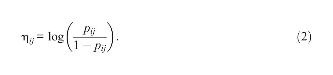
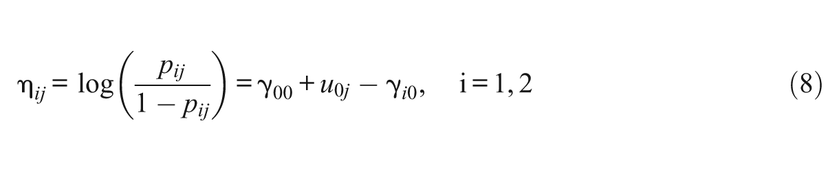
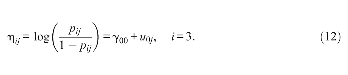
In general, there are three popular model identification methods, both in single-group and multiple-group conditions. Because readers might be more familiar with that under the IRT framework, the authors show how to form the Rasch model as a HGLM. Let pij be the probability of success on item i for person j. Under the Rasch model, the log odds of a correct answer over an incorrect answer are defined as

where θ
j
is the latent trait of person j and δ
i
is the difficulty of item i. There are three elements in HGLM: a probability distribution from the exponential family, a link function, and a linear predictor at each level. To form the Rasch model as a HGLM, a two-level model should be created where Level 1 is the item response level and Level 2 is the person level. The response of person j (
At Level 1 (item level), the linear predictor is

where
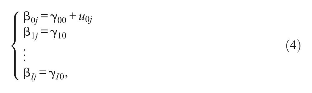
where
Equations 3 and 4 are not identifiable without constraint. If the Rasch model is to be formed using Equations 3 and 4, one constraint has to be made. In the Rasch model, either the mean of the person ability is fixed at a value (e.g., zero) or the mean of the item difficulty is fixed at a value (e.g., zero). Where appropriate (e.g., in linking design), the difficulty of an item (e.g., the last item) can be fixed at a value (e.g., zero). Below, the authors show how to set these three kinds of constraints by specifying the design matrix
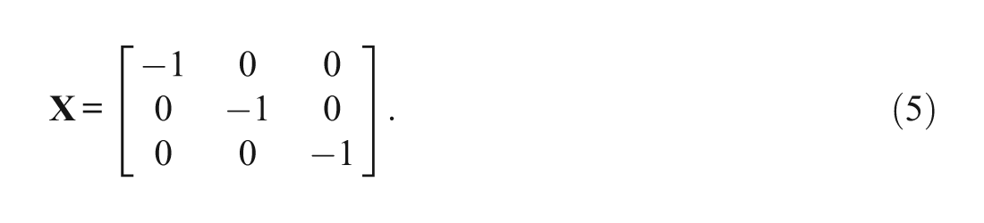
With γ00 = 0 and Equation 5, Equations 2 through 4 can be combined as
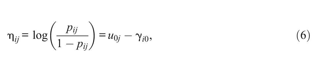
where γ10 is the difficulty of Item 1, γ20 is the difficulty of Item 2, and γ30 is the difficulty of Item 3.
When the mean item difficulty is assumed to be zero, γ00 can be freely estimated, and it depicts the mean ability. The design matrix should be set as

With this design matrix, Equation 3 becomes

In other words, γ00 is the mean ability, γ10 is the difficulty of Item 1, γ20 is the difficulty of Item 2, and −(γ10+γ20) is the difficulty of Item 3.
When the difficulty of the last item is assumed to be zero, γ00 can be freely estimated, and it depicts the mean ability. The design matrix should be set as
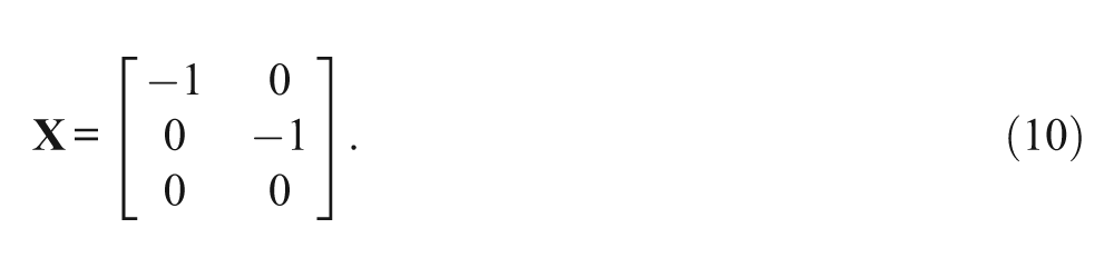
With this design matrix, Equation 3 becomes

That is, γ00 is the mean ability, γ10 is the difficulty of Item 1, γ20 is the difficulty of Item 2, and the difficulty of Item 3 is zero.
DIF Assessment With the HGLM
Let Gj be the group membership for person j. For simplicity, let there be two groups: one is the reference group (Gj = 0), and the other is the focal group (Gj = 1). To assess DIF, the regression coefficient can be set as

Again, the three-item test is taken as an example. When the mean ability is assumed to be zero for both groups (i.e., γ00 = γ01 = 0), the design matrix should be set as Equation 5. Thus, γ10 is the difficulty of Item 1 for the reference group, γ10+γ11 is the difficulty of Item 1 for the focal group, γ20 is the difficulty of Item 2 for the reference group, γ20+γ21 is the difficulty of Item 2 for the focal group, γ30 is the difficulty of Item 3 for the reference group, and γ30+γ31 is the difficulty of Item 3 for the focal group. In this setting, γ11 reflects the DIF size for Item 1, γ21 reflects the DIF size for Item 2, and γ31 reflects the DIF size for Item 3. In other words, all items can be assessed for DIF, at the cost of the assumption of equal mean ability between groups. This assumption may not hold in practice, especially in cognitive tests for majority and minority groups. It can be predicted that the more the reference and focal groups differ in mean ability, the worse the performance of DIF assessment based on this equal mean ability assumption, which is called the equal mean ability method (Wang, 2004), and Williams and Beretvas (2006) used this method to identify a HGLM.
When the mean item difficulty is assumed to be zero for both groups, the mean abilities for both groups can be freely estimated, and the design matrix should be set as Equation 7. Thus, γ00 is the mean ability for the reference group, γ00+γ01 is the mean ability for the focal group, γ10 is the difficulty of Item 1 for the reference group, γ10+γ11 is the difficulty of Item 1 for the focal group, γ20 is the difficulty of Item 2 for the reference group, γ20+γ21 is the difficulty of Item 2 for the focal group, −(γ10+γ20) is the difficulty of Item 3 for the reference group, and −(γ10+γ20) − (γ11+γ21) is the difficulty of Item 3 for the focal group. This method is referred to as the equal mean difficulty method (Wang, 2004), and Luppescu (2002) used this method to identify the HGLM. When there is a single DIF item in a test, by definition, the equal mean difficulty method is not appropriate. Even if there are multiple DIF items in a test, it is not likely that the DIF sizes will be balanced (symmetric) between groups such that the mean item difficulties are equal between groups. Only when the test does not have any DIF item or the DIF sizes are balanced, will this method be appropriate. The worse the balance, the worse the method will perform (Wang, 2004).
When the difficulty of an item (e.g., the last item) is assumed to be zero for both groups, the mean abilities for both groups can be freely estimated, and the design matrix should be set as Equation 10. It can be shown that γ00 is the mean ability for the reference group, γ00+γ01 is the mean ability for the focal group, γ10 is the difficulty of Item 1 for the reference group, γ10+γ11 is the difficulty of Item 1 for the focal group, γ20 is the difficulty of Item 2 for the reference group, γ20+γ21 is the difficulty of Item 2 for the focal group, and the difficulty of Item 3 for both groups is, by design, zero. This method is referred to as the constant item (CI) method (Wang, 2004) because when assessing items for DIF, a fixed item (or a set of fixed items) is set as DIF-free. This method has been adopted to identify the HGLM in Cheong (2006). If the fixed (anchored) item (Item 3 in this example) is indeed DIF-free, this method will perform appropriately. However, if the fixed item has DIF, then this method will perform inappropriately.
According to the preceding description as the identification of equal mean ability and equal mean difficulty are both unrealistic when applying the HGLM in DIF assessment, the focus of the question in this study is switched to the identification of CI method. When assessing DIF with the CI method, a set of DIF-free items were used to anchor the scales for different groups. An anchored scale in this way is quite similar to the one that assesses DIF with the MIMIC method, where the factor loading of the first item (i.e., the reference item) is constrained to 1 for both groups. After the reference item was selected, all other items in the test, except for the reference item, were taken as the studied item and were assessed for DIF on the common metric. Through a simulation, the CI method was found to yield well-controlled Type I error rates in assessing DIF, even when 40% items of the test are DIF items, given that the anchor is indeed pure (i.e., DIF-free; Shih & Wang, 2009; Wang & Yeh, 2003). By setting one DIF-free item as reference for identifying the HGLM, the equal mean ability constraint can be released, and the DIF assessment can proceed correctly, given the reference item is indeed DIF-free. Though the CI method has been adopted in Cheong (2006), the reference items were arbitrarily selected. Accordingly, the question is further transformed into how to select a DIF-free item first and then conduct DIF analysis using the HGLM with the CI method. Methods that can be used to select reference items for the CI method will be introduced later. Setting these items as reference items, the CI method can be used to assess DIF for items. Combining the two procedures where selecting the most likely DIF-free items as reference first and then assessing DIF for other items in the test, the new DIF assessment strategy is called the DIF-free-then-DIF (DFTD; Wang, Shih, & Sun, 2012). Though the DFTD strategy is new, it has been applied to the MIMIC method and the likelihood ratio test method (Shih & Wang, 2009; Wang et al., 2012; Wang & Shih, 2010). However, because both MIMIC and likelihood ratio test did not take the data structure into consideration, ignoring the multilevel data structure may result in a substantial inflation of Type I error rates in assessing DIF (French & Finch, 2010). Therefore, the effect of applying the DFTD strategy to the HGLM to assess DIF, as well as the performances of different methods in selecting DIF-free items, was investigated under various conditions through a series of simulations in this study.
This study is organized as follows. First, the reference item selection method and the DFTD strategy are introduced. Second, the authors discuss how they apply the DFTD strategy to the HGLM, including both steps of selecting DIF-free items and then assessing DIF with the CI method. Third, two simulation studies are conducted to explore the performance of applying the HGLM in selecting DIF-free items and using previously identified DIF-free items as anchors to assess other items for DIF. Finally, the results are reported, and then conclusions are drawn.
Reference Item Selection Method and DFTD Strategy
The CI method establishes a common metric for the groups by anchoring one or several items as the reference and then assessing DIF for other items in the test by assuming these reference items are DIF-free. To assess DIF with the likelihood ratio test method, Wang and Yeh (2003) conducted a simulation study to compare the performance of the CI method and the all-other-item (AOI) method. The results showed that the CI method performed better than the AOI method in controlling the Type I error rate and increasing power rate given the anchor was indeed DIF-free. By introducing the iterative CI method to select the most likely DIF-free items as reference, Shih and Wang (2009) recommended the CI method should be used to assess DIF for items for the method’s good control over Type I error rates.
To correctly select DIF-free items as the reference for the DFTD strategy, two methods derived from DIF assessment methods have been proposed in the literature (Shih & Wang, 2009; Woods, 2009). For the first one, the CI method was used iteratively to assess DIF for items and then select a set of items that are most likely to be DIF-free as an anchor. This so-called iterative constant item (ICI) method (Shih & Wang, 2009) contains the following steps:
Set Item 1 as the reference and assess all other items in the test for DIF using the CI method with one-item reference. Estimate the DIF effect for each studied item.
Set the next item as the reference and assess all other items in the test for DIF using the CI method with a one-item reference. Estimate the DIF effect for each studied item.
Repeat Step 2 until the last item is set as the reference item.
Compute the mean absolute values of the DIF effects for each item over all iterations and select the item that has the smallest mean absolute value as DIF-free.
The ICI method was successfully applied to the MIMIC method and yielded nearly perfect accuracy in selecting one DIF-free item, especially when the sample sizes of the two groups are large, for example, both groups contain 1,000 examinees (Shih & Wang, 2009). In applying this method to the HGLM, this new method for selecting reference items is called H-IT (HGLM method with ICI strategy).
The second method, called rank-based strategy, was proposed by Woods (2009) and has been applied to the likelihood ratio test method. Through a simulation, Woods found that the rank-based strategy could almost always select a DIF-free reference item set when there were 20% to 50% DIF items in the test. Because the procedure for the rank-based strategy contains the original DIF assessment procedure of the likelihood ratio test, and Woods stated that the strategy was applicable to any other DIF assessment method, the strategy could be applied to the HGLM with an original procedure that assumes the mean ability is zero for both groups. This new application is called H-OR (original HGLM method).
The DFTD strategy has been applied to the MIMIC method and the likelihood ratio test method and yielded satisfying results (Shih & Wang, 2009; Wang et al., 2012; Wang & Shih, 2010). Furthermore, Chen, Chen, and Shih (2010) explored the performance of the DIF assessment using the HGLM and indicated it was appropriate for assessing DIF. In addition, they found that using DIF-free items to serve as references for assessing DIF within the HGLM can yield high power rates and well-controlled Type I error rates. Based on the findings, the DFTD strategy is combined with the HGLM method in this study. To select DIF-free items as the reference, H-IT and H-OR were examined, and their performances were compared through simulation. To better understand the difference between H-IT and H-OR, a test that contains k items is used as an example.
In the H-IT method, DIF assessment with the CI method should be carried out k times by setting each item as the reference iteratively. Except for when the item is itself a reference, each item is assessed for DIF k– 1 times, and the DIF effects are estimated and then recorded. After the absolute values of the DIF effects across iterations are averaged, the item with the lowest value on the DIF effect is deemed DIF-free and then identified as the reference for the following DIF assessment. In the H-OR method, the original HGLM procedure for DIF assessment is implemented, and the item with the least value on the DIF effect is selected as the reference. The two methods should perform similarly when there is no impact, whereas the H-IT method should perform better (i.e., with higher accuracy) in selecting DIF-free items than the H-OR when there is a nonignorable impact.
In this study, the DFTD strategy is applied to the HGLM, and its performance is evaluated through simulation studies. Because investigating the effect of the number of reference items in DIF assessment is an important issue for researchers and practitioners, the efficiency of assessing DIF between the one- and four-reference-item CI methods is also compared. Two anchor lengths were considered because one- and four-reference items were suggested by Woods (2009) and Shih and Wang (2009), respectively. When the HGLM is applied to DIF assessment, reference items are used to anchor the scale of the latent trait for two groups. The quality of the scale being linked with the four-reference item would be better than for that with one-reference item if all the reference items are DIF-free. However, the possibility of including DIF items in the reference set is also higher for the four-reference-item condition than for the one-reference-item condition. There is a trade-off between the quality of the scale linking and the accuracy of selecting all DIF-free items as the reference.
Another DIF assessment strategy that contains multiple steps is the scale purification (SP) procedure (Lord, 1980). The SP procedure improves the performance of the DIF assessment by iteratively relinking the matching scale that consists of the items assessed as DIF-free in a previous iteration and then assesses DIF for all items in this iteration. Most SP procedures consist of the following major steps (Wang, Shih, & Yang, 2009): (a) initially assessing DIF for all items, (b) removing those items that are assessed as exhibiting DIF from the matching variable, (c) reassessing DIF for all items, and (d) repeating steps (b) and (c) until the same set of items are assessed as exhibiting DIF in two consecutive iterations. For readers who are familiar with the SP procedure and its extensions (Candell & Drasgow, 1988; Holland & Thayer, 1988; Park & Lautenschlager, 1990), the DFTD strategy is different from the SP procedure in at least two ways. First, the matching variable used to match examinees of different groups and estimate ability parameters is different in the DFTD and the SP procedure. Based on different length of matching variable, the ability estimates could be different, and therefore, it is expected to affect Type I error and power rates of DIF assessment for DFTD and SP procedure, respectively. In the DFTD strategy, the matching variable contains a fixed number of items (i.e., all items in the test), whereas in the SP procedure the length of the matching variable varies and depends on whether the studied item is exhibiting DIF. All items assessed as DIF in the previous iteration should be removed from the matching variable in the current iteration. The only exception is that the studied item is always involved in the matching variable no matter it is exhibiting DIF or not. Taking a 20-item test for example, assume that Items 1, 2, and 3 were assessed as DIF items in the first iteration (i.e., the original DIF assessment procedure). If the SP procedure is adopted, the number of items contained in the matching variable varies in the second iteration. When assessing DIF for Items 1 to 3, the matching variable contains 18 items (Items 4-20, which were deemed DIF-free in the first iteration, plus the studied item), whereas the matching variable contains 17 items (Items 4-20) when Items 4 to 20 were being assessed for DIF. However, when DFTD is adopted, the matching variable always contains 20 items, both in the selection of DIF-free items as the reference and the following DIF assessment.
Second, the logic of DIF assessment is different between the DFTD strategy and the SP procedure. In the DFTD strategy, after the items have been selected as the reference, they (the reference items) are deemed DIF-free and are not assessed for DIF in the DFTD procedures that follow. Setting these DIF-free items as the reference, all other items are assessed for DIF only once, and the results are taken as the outcome of the DFTD strategy. However, every item is continuously being assessed for DIF in every iteration of the SP procedure (i.e., step (c) of SP procedure) until the same set of items is deemed DIF in two consecutive iterations. According to the authors’ experiences, each item is on average assessed for DIF about 4 times in the SP procedure but only 2 times in the DFTD strategy, one for selecting DIF-free items as the reference and the other for the following DIF assessment.
Method
The main goal of this study is to apply the DFTD strategy to the HGLM in assessing DIF and to compare the strategy’s performance with an original HGLM. To implement the DFTD strategy, two methods for selecting reference items were used: H-IT and H-OR. After the comparison, the method with higher accuracy in selecting DIF-free items was then used to select the reference item for the CI method while proceeding with the following DIF assessment (called H-DFTD [HGLM method with DFTD strategy]). In addition, H-OR was applied to assess all test items for DIF without the DFTD strategy, and this was regarded as a baseline to show the improvement in applying the DFTD strategy to the HGLM in assessing DIF.
Simulation Study 1
The purpose of Simulation Study 1 was to compare the accuracy in selecting DIF-free items. Five independent variables were manipulated in this simulation study: (a) the amount of impact: 0 and 0.5; (b) the number of reference items to be selected: 1 and 4 items; and (c) the DIF pattern: constant and balanced. For the constant DIF pattern, all the DIF items favored the same group (usually the reference group), whereas one half of DIF items favored one group and the other half favored another group in the balanced pattern; (d) the percentage of DIF items: 0%, 20%, and 40%; and (e) sample size: R500/F250, R250/F250, and R250/F150, where R and F represented the reference and focal groups, respectively. The purpose for manipulating these independent variables is listed in the following.
Impact
Mean ability differences are common among groups in real data, and it can interact with other variables and degraded power rates of DIF assessment (Jodoin & Gierl, 2001). In addition, the Type I error rates tended to be inflated when there exists mean ability difference between groups (DeMars, 2010). Furthermore, the main difference between the two methods (H-OR and H-DFTD) is expected to be found when impact existed. Therefore, impact was manipulated in this study. The impact was set at 0 for the no difference in mean ability between groups, whereas 0.5 was chosen to represent the largest difference between genders in the literature reviewed in this study (Willingham & Cole, 1997).
Number of Reference Items
The number of reference items in DIF assessment was investigated in many studies and the recommended number is different across studies (Shih & Wang, 2009; Thissen et al., 1988; Wang & Yeh, 2003; Woods, 2009). A four-item reference is generally recommended but single reference item is also recommended for large sample size. To investigate how many reference items should be used in H-DFTD to yield a satisfying performance in assessing DIF, various lengths of reference items suggested in the literature (Shih & Wang, 2009; Woods, 2009) were manipulated in this study.
DIF Pattern
The DIF pattern was manipulated for the balanced and constant conditions to depict the most fair and most unfair situations, respectively, given the percentage of DIF items held fixed. In real tests, the DIF patterns may fall between the two extremes of DIF patterns; that is, most DIF items favor the reference group. The results obtained from these two extremes enable appropriate inferences (Wang et al., 2012). Therefore, this variable is manipulated in this study, as well as in many other studies (Ankenmann, Witt, & Dunbar, 1999; Chang, Mazzeo, & Roussos, 1996; Gierl, Gotzmann, & Boughton, 2004; Shih & Wang, 2009; Wang & Su, 2004; Wang & Yeh, 2003; Zwick, Donoghue, & Grima, 1993).
Percentage of DIF Items
Large percentage of DIF items can reduce the validity of the matching variable and result in less accurate ability estimates, therefore it is expected to affect Type I error and power rates of DIF assessment (French & Maller, 2007; Jodoin & Gierl, 2001). Consequently, this variable is manipulated here, as well as in many other studies (Shih & Wang, 2009; Wang et al., 2012; Wang & Yeh, 2003).
Sample Size
Type I error and power rates for many DIF assessment methods were increased as sample size of the reference and focal groups increased (Jodoin & Gierl, 2001; Narayanan & Swaminathan, 1994; Rogers & Swaminathan, 1993; Roussos & Stout, 1996). Besides, the authors wanted to know if the methods investigated in this study performed well when the sample size is relatively small, which can help practitioners know how many samples should be drawn if they want to assess DIF with this method.
The dependent variable is the accuracy of selecting DIF-free items. When four-reference items were selected, the accuracy was 0.25, 0.50, 0.75, and 1.00, respectively, as 1, 2, 3, and 4 of the selected items were indeed DIF-free. To fully implement the DFTD strategy in the HGLM, the method with higher accuracy rate in selecting DIF-free items was then used to select reference items for the HGLM method and then assess DIF for other items by setting these selected items as the reference.
Simulation Study 2
The purpose of Simulation Study 2 was to compare the performance of the DIF assessment between the original HGLM method and the H-DFTD method. The independent variables were identical to those in Simulation Study 1, whereas the dependent variables were Type I error rates and power rates of DIF assessment.
In Studies 1 and 2, the abilities of examinees in the reference group were sampled from standard normal distribution, whereas those of the focal group were sampled from N(−0.5, 1) and N(0,1) when the impact was set at 0.5 and 0, respectively. The test length was set to be 30 items to mimic a general medium length test. Item parameters were taken from Cohen, Kim, and Wollack (1996), in which difficulty parameters ranged from −2.28 to 1.51, with a mean of −0.53 and a standard deviation of 1.16. The DIF amount for each item was sampled from a normal distribution with mean and variance equal to 0.6 and 0.01, respectively.
The data in the simulation study were generated according to the Rasch (1960) model using a Fortran 6.6.0 computer program written by the authors with 100 replications for each condition. The replication was set at 100 for the outcomes of the simulations are quite similar to the outcomes with 200 replications in the authors’ pilot study, and 100 replications are relatively larger than the 50 replications adopted in previous HGLM studies (Luppescu, 2002; Williams & Beretvas, 2006). The parameter estimation and corresponding DIF assessment of HGLM were implemented with the software HLM 6.02 (Raudenbush, Bryk, & Congdon, 2005).
Results
Study 1: Accuracy of Selecting DIF-Free Items Using H-OR and H-IT
The accuracies of selecting DIF-free items using H-OR and H-IT are summarized in Table 1. When the impact is zero, both methods performed fairly well in selecting DIF-free items. The accuracies ranged from 0.90 to 1.00 and in general increased as (a) the percentage of DIF items in the test decreased, (b) the sample size increased, (c) fewer DIF-free items were selected, and (d) the DIF pattern was balanced. When impact was equal to 0.5, the accuracy of H-IT was almost the same as with the no-impact condition, whereas the accuracy for H-OR decreased remarkably, especially when the DIF pattern was balanced. The accuracies of H-OR ranged from .77 to .93 and .19 to .68 for the constant and balanced conditions, respectively. However, H-IT yielded nearly perfect accuracy (no less than .90) in selecting one- or four-reference items, no matter what the DIF pattern was. In summary, the H-IT method is recommended for selecting DIF-free items within the HGLM framework for superior performance across various conditions.
Accuracy of Selecting DIF-Free Items Using H-IT and H-OR.
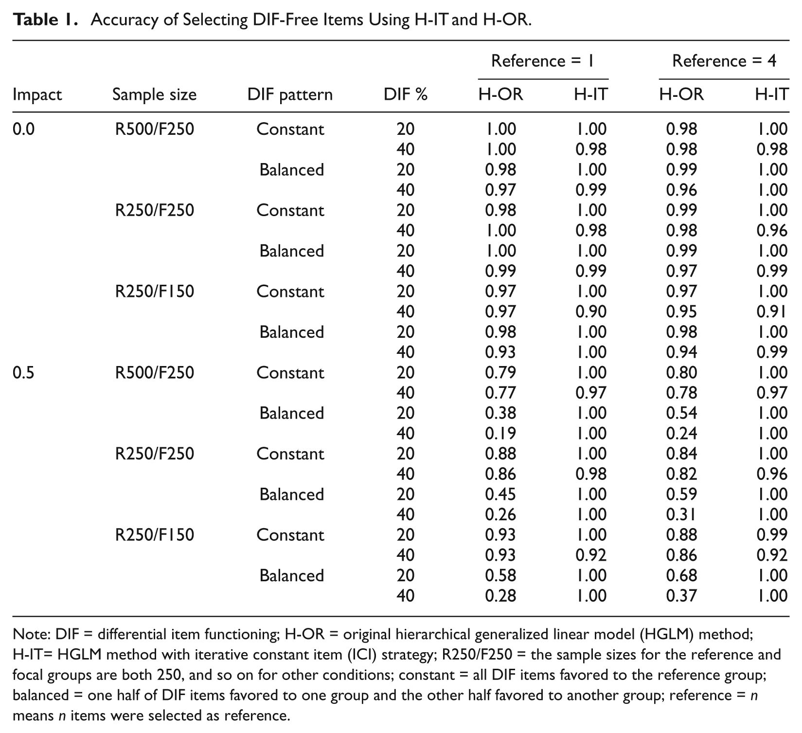
Note: DIF = differential item functioning; H-OR = original hierarchical generalized linear model (HGLM) method; H-IT= HGLM method with iterative constant item (ICI) strategy; R250/F250 = the sample sizes for the reference and focal groups are both 250, and so on for other conditions; constant = all DIF items favored to the reference group; balanced = one half of DIF items favored to one group and the other half favored to another group; reference = n means n items were selected as reference.
Study 2: Outcomes of DIF Assessment Using H-OR and H-DFTD
Through the results of Simulation Study 1, the H-IT method outperformed the H-OR method in selecting DIF-free items as the reference. Therefore, the H-IT method was adopted in Simulation Study 2 to select reference items for the H-DFTD method. Results of Simulation Study 2 were divided into two parts and listed in Tables 2 and 3 for impact equal 0 and 0.5, respectively. Within these two tables, inflated mean Type I error rates and their corresponding power rates are given in italics. A conservative criterion of Type I error rate of 0.10 was used in this study, that is, Type I error rates higher than 0.10 would be taken as inflated.
Type I Error Rates and Powers of DIF Assessment Using H-OR and H-DFTD for Conditions With the Impact = 0.
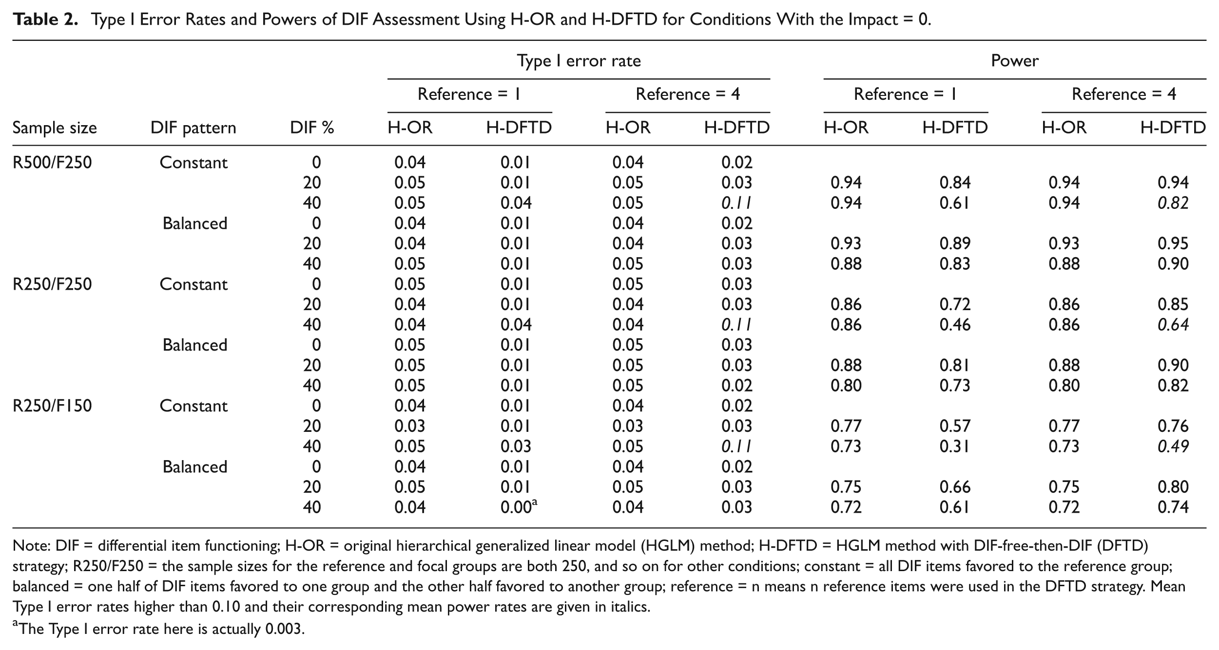
Note: DIF = differential item functioning; H-OR = original hierarchical generalized linear model (HGLM) method; H-DFTD = HGLM method with DIF-free-then-DIF (DFTD) strategy; R250/F250 = the sample sizes for the reference and focal groups are both 250, and so on for other conditions; constant = all DIF items favored to the reference group; balanced = one half of DIF items favored to one group and the other half favored to another group; reference = n means n reference items were used in the DFTD strategy. Mean Type I error rates higher than 0.10 and their corresponding mean power rates are given in italics.
The Type I error rate here is actually 0.003.
Type I Error Rates and Powers of DIF Assessment Using H-OR and H-DFTD for Conditions With the Impact = 0.5.
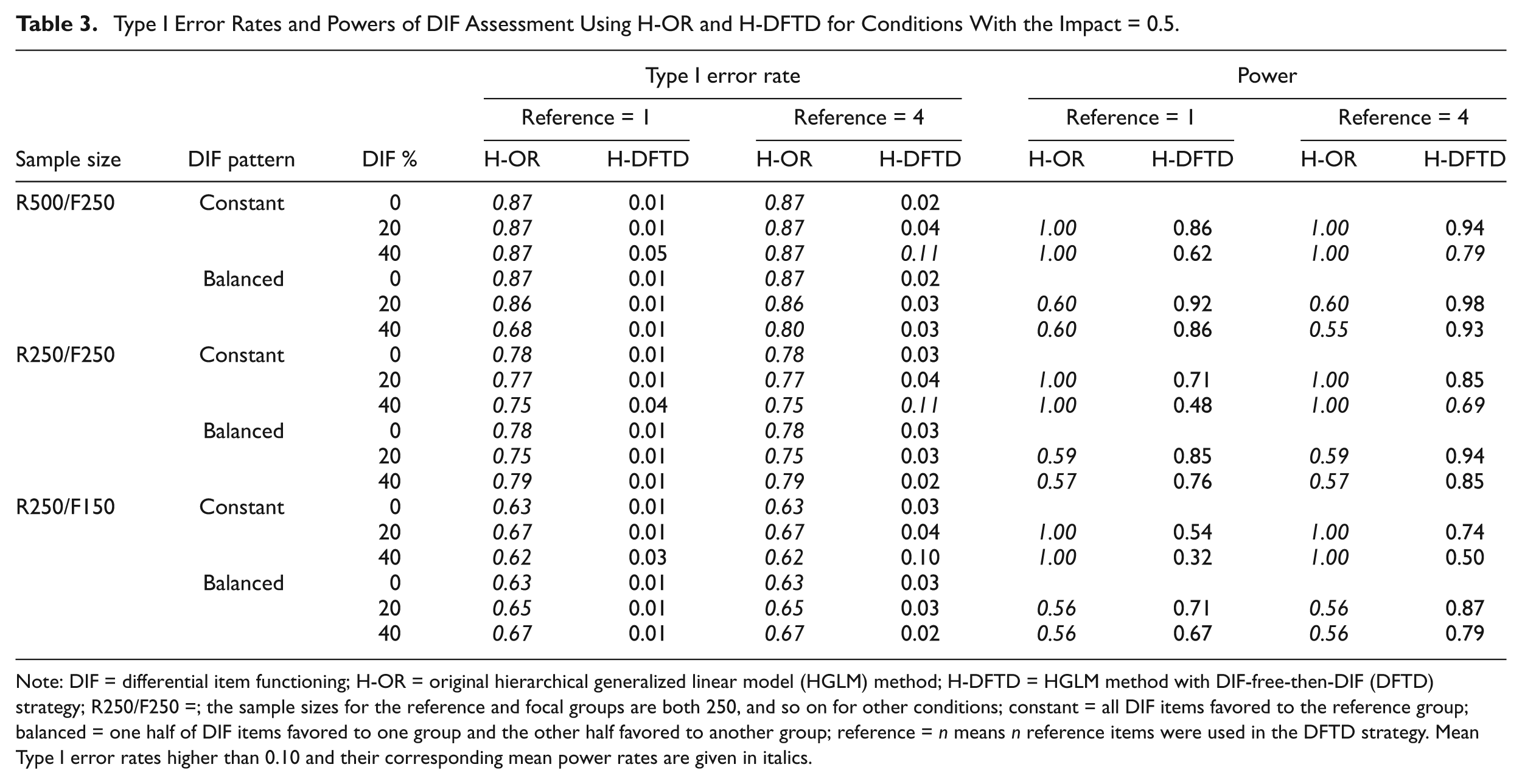
Note: DIF = differential item functioning; H-OR = original hierarchical generalized linear model (HGLM) method; H-DFTD = HGLM method with DIF-free-then-DIF (DFTD) strategy; R250/F250 =; the sample sizes for the reference and focal groups are both 250, and so on for other conditions; constant = all DIF items favored to the reference group; balanced = one half of DIF items favored to one group and the other half favored to another group; reference = n means n reference items were used in the DFTD strategy. Mean Type I error rates higher than 0.10 and their corresponding mean power rates are given in italics.
Impact = 0
The mean Type I error rates and power rates of DIF assessment across replications under the no-impact conditions are listed in Table 2. The Type I error rates for H-OR were well controlled under all conditions (ranging from .03 to .06). For H-DFTD, the Type I error rates were conservative yet acceptable under most conditions (ranging from .003 to .03), but slightly inflated (.11) when using four-reference items on the test contained 40% DIF items and all favored the same group, across various sample sizes for both groups. Referring to Table 1, the accuracy under these conditions was slightly lower than 1.00 (ranging from 0.91 to 0.98), which caused incorrectly selected DIF items as the anchor, and therefore inflated the Type I error rates of the following DIF assessment procedure.
The power rates increased as the sample size increased and the DIF percentages decreased. Moreover, for the H-DFTD method, the power rates under balanced DIF pattern were higher than those under constant DIF pattern. Comparing the performance of the two methods showed that the power rates for H-OR were slightly higher than for H-DFTD, especially under the one-reference-item conditions. The only exception was using the four-reference item under balanced pattern conditions. As to the effect of anchor length, there was no difference between the one-reference item and the four-reference item for the H-OR method, whereas the H-DFTD method yielded higher power rates and reasonable Type I error rates under the four-reference-item conditions.
Impact = 0.5
The mean Type I error rates and power rates of the DIF assessment across replications when the impact was 0.5 are summarized in Table 3. The Type I error rates and the power rates for H-DFTD were similar to those under no-impact conditions. However, the Type I error rates for H-OR were highly inflated (ranging from .62 to .87) for the one- and four-reference-item conditions, and therefore, the corresponding power rates, even as higher as 1.00 in several conditions, are meaningless. As the power rates were meaningless when Type I error rates were out of control, the H-DFTD seemed to be the only reasonable choice under these conditions. In light of the results shown in Table 3, H-DFTD can maintain well-controlled Type I error rates under nonzero impact conditions with satisfactory power, whereas the H-OR method performed poorly in maintaining Type I error rates.
Discussion and Conclusion
Several multilevel formulations of IRT models have been proposed in the literature (Adams, Wilson, & Wang, 1997; Hedeker & Gibbons, 1993; Spiegelhalter, Thomas, Best, & Gilks, 1996). Treating the item response model in this way, the hierarchical structure presented in the data can be better handled, which was not taken into account in the IRT models. Because the two-level item analysis model has been shown to be algebraically equivalent to the Rasch model, issues such as dimensionality, rater effect, and DIF assessment can be easily handled by the HGLM. Furthermore, predictors for investigating the possible sources for DIF can be added to the model due to the flexibility of the HGLM, which cannot be done in IRT models.
Three ways for identifying an HGLM were introduced in this study. However, assessing DIF with the HGLM that adopted equal mean ability (Williams & Beretvas, 2006) or equal mean difficulty (Luppescu, 2002) to identify the model is not reasonable in reality. As this assumption is not reasonable and hardly held in multiple-group issues, another option was suggested. By applying the DFTD strategy to the HGLM method, a set of items that are most possibly DIF-free should be selected first and can be set as the reference for the following DIF assessment. Because the DIF-free reference item can be selected with perfect or nearly perfect accuracies, the CI method should be used to identify the HGLM, and therefore, DIF assessment can be implemented accordingly. This DFTD strategy is somewhat different from the well-known SP procedure. However, the SP procedure should not be applied to HGLM due to technical considerations. The computational burden is heavy when using HLM 6.02 (Raudenbush et al., 2005) for many replications, especially for the SP procedure. More specifically, a common analysis in software HLM needs two distinct syntax files: one is used to create an .MDM file for analysis, and the other is used to specify the model for analyzing the data and other related settings. Within the SP procedure, items that are deemed DIF usually differ across the first several iterations, and the DIF assessment procedure then keeps processing. Under these conditions, both syntax files must be modified to perform a DIF assessment. This results in great complexity in syntax modification and causes difficulty for practitioners in applying the SP procedure to the HGLM.
A series of simulations was conducted in this study to investigate the accuracies of selecting DIF-free items using two methods under the HGLM framework, and then the efficiency of the DIF assessment was examined by setting these items as the reference. The results showed that the HGLM with the ICI method performed quite well in selecting DIF-free items as well as in assessing DIF items regardless of the existence of impact, whereas the H-OR method correctly selected DIF-free items only when there was no impact between the groups. H-OR performed poorly in selecting DIF-free items as the reference under the balanced condition when impact existed. This is because by applying the equal mean ability method under the balanced condition, the mean ability of the focal group, as well as all item parameters, should be shifted by 0.5 logit to maintain the relative position between the items and the mean ability. Thus, the magnitude of DIF for DIF items that favored the focal group would be −0.5 logit accordingly. They then became the items nearest the mean ability and tended to be mistakenly selected as the reference after the shift. Therefore, all DIF-free items and DIF items that favored the reference group were then assessed as DIF items, which caused inflated Type I error rates, and only half of the DIF items (favored to the reference group) were correctly deemed DIF. This is consistent with the fact that the power rates are close to .50 under the balanced conditions in Table 3. By setting these items as reference and then assessing DIF with the CI method, the power increased as the number of reference items and sample size increased. In summary, for readers who want to assess DIF with the HGLM method, the DFTD strategy is strongly recommended for yielding well-controlled Type I error rates and higher power rates than the H-OR method did. Furthermore, the advantages of applying the HGLM in the DIF assessment, such as the capability of handling hierarchical data, are available due to the procedures for assessing DIF established in this study.
To implement the HGLM and all methods discussed in this study, researchers and practitioners can use the software HLM to help estimate all the parameters. For those who are more familiar with R language (R Development Core Team 2011), the HGLM has been incorporated into R, and a package called HGLMMM was recently developed that might be another choice. Detailed information can be found in Molas and Lesaffre (2011).
Several issues remain unclear and need further investigation. First, the Type I error rates for H-DFTD seemed overly conservative under most of the conditions, and were not found in other studies that used the HGLM for DIF assessment (Kamata, 1999; Williams & Beretvas, 2006). Second, extending this study to polytomous or multidimensional scales, which are used in many social and behavioral domains to improve the application of the DIF assessment using the HGLM, is essential. Third, investigating the performance of H-DFTD in selecting various DIF items and assessing possible sources simultaneously would be beneficial. By adding item covariates to the model, the specific source of the difficulty can be considered in the model, and therefore, the DIF source can be explained by specific item covariates (Van den Noortgate & De Boeck, 2005). Finally, the scale indeterminacy issue, DIF assessment, and item purification in generalized linear mixed models (GLMM) has been investigated recently (Cheong & Kamata, 2013; Liu, 2011); the effect of DFTD in GLMM can be also further investigated.
Footnotes
Declaration of Conflicting Interests
The authors declared no potential conflicts of interest with respect to the research, authorship, and/or publication of this article.
Funding
The authors disclosed receipt of the following financial support for the research, authorship, and/or publication of this article: Ching-Lin Shih was supported by a grant from the National Science Council of Taiwan (NSC 100-2410-H-110-015).