A Numerical Investigation of the Recovery of Point Patterns With Minimal Information

Backbone Algorithm

The algorithm, outlined below, is described by Levine and Kreifeldt (1994). It recursively builds an adjacency matrix for a graph possessing n vertices (points). An n×n adjacency matrix is a binary matrix with entry (i,j) being 1 if vertices i and j are connected, and 0 otherwise. The retained dissimilarities are indicated by a value of 1 in the adjacency matrix. The algorithm develops an n vertex graph from an n − 1 vertex graph for all n≥5. Note that the complexity of determining which edges (branches) to add and to remove does not increase as n increases.

Because the identification of the points is arbitrary, relabeling the vertices allows for n! isomorphs of each graph, each giving rise to a different set of desired dissimilarities.

The advantages of using the backbone are twofold. The volume of the data collection task can be vastly reduced. In the backbone case, the number of dissimilarities required, for n > 3 and n odd, there are ½(3n + 1) dissimilarities, while if n is even there are ½3n (Levine & Kreifeldt, 1994), compared with ½n(n − 1) for the full set of dissimilarities.

In addition, when, for example, evaluating the stress in nonmetric MDS (Cox & Cox, 2001), only the available dissimilarities need be considered. The computational effort is thus greatly reduced.

The “degrees of freedom” ratio is the ratio of the number of dissimilarities that would remain for a given percentage to the “degrees of freedom” of the coordinates, m(n− 1) − ½m(m − 1), where there are n points in m dimensions (here m = 2). Spence and Domoney (1974) reported that recovery of the original configuration was found to be satisfactory provided that the “degrees of freedom” ratio exceeded 3.5, irrespective of error level. With zero error, this ratio should exceed about 2.5 for good recovery and with moderate and high levels of error, the respective values are about 3.0 and 3.5. Young (1970) found that, with complete data, if the ratio exceeded about three, metric recovery was acceptable even with the highest levels of error. The study of Spence and Domoney confirms that this rule of thumb holds approximately in the context of incomplete data. Although their results may be extrapolated quite safely to larger numbers of points, they may not hold for configurations with fewer than 30 points.

It is often necessary to compare a configuration of points in one Euclidean space with another, where there is a one-to-one mapping between the sets of points. The technique of matching one configuration to another and producing a measure of the match is called Procrustes analysis. Procrustes analysis seeks the isotropic dilation and the rigid translation, reflection, and rotation needed to best match one configuration to the other (for further details, see Mardia, Kent, & Bibby, 1979; Sibson, 1979).

The remaining sections use the backbone procedure; first, the breakfast cereal data (Cox & Cox, 2001) is used. This data set was introduced for the 1993 Statistical Graphics Exposition organized by the American Statistical Association. It was proposed for analysis by interested people and could be presented at the Annual Meeting of the Association. For clarity of graphical illustration, only those breakfast cereals manufactured by Kellogg are analyzed here, reducing the number of cereals to 23. This example is of a similar size to the caffeine molecule problem (n = 24) considered by Tsogo et al. (2001). This will provide a direct indication of the effect of removing available information as the suggested backbone is approached.

Does Reduction to the Backbone Dissimilarities Affect the Solution?

The calculation commences with the full data set. To investigate the effect of removing dissimilarities, a selected backbone is identified. Successive redundant dissimilarities, which are not in this backbone, are randomly removed, and the resulting matrix of dissimilarities is analyzed using nonmetric MDS. For ease of computation, a 2D solution is considered.

Initially, a random 2D vector associated with the full set of points is generated and the standard MDS procedure (Kruskal, 1964; Lingoes & Roskam, 1973) used. At each stage, the last solution vector obtained provides a starting point for the calculation. The initial solution vector is retained and compared with successive solutions, which are obtained as dissimilarities are removed, a Procrustes statistic being used to make this comparison. The results are presented in Figures 1 and 2.

OPEN IN VIEWER

Figure 1.

2D stress with successive dissimilarities excluded

OPEN IN VIEWER

Figure 2.

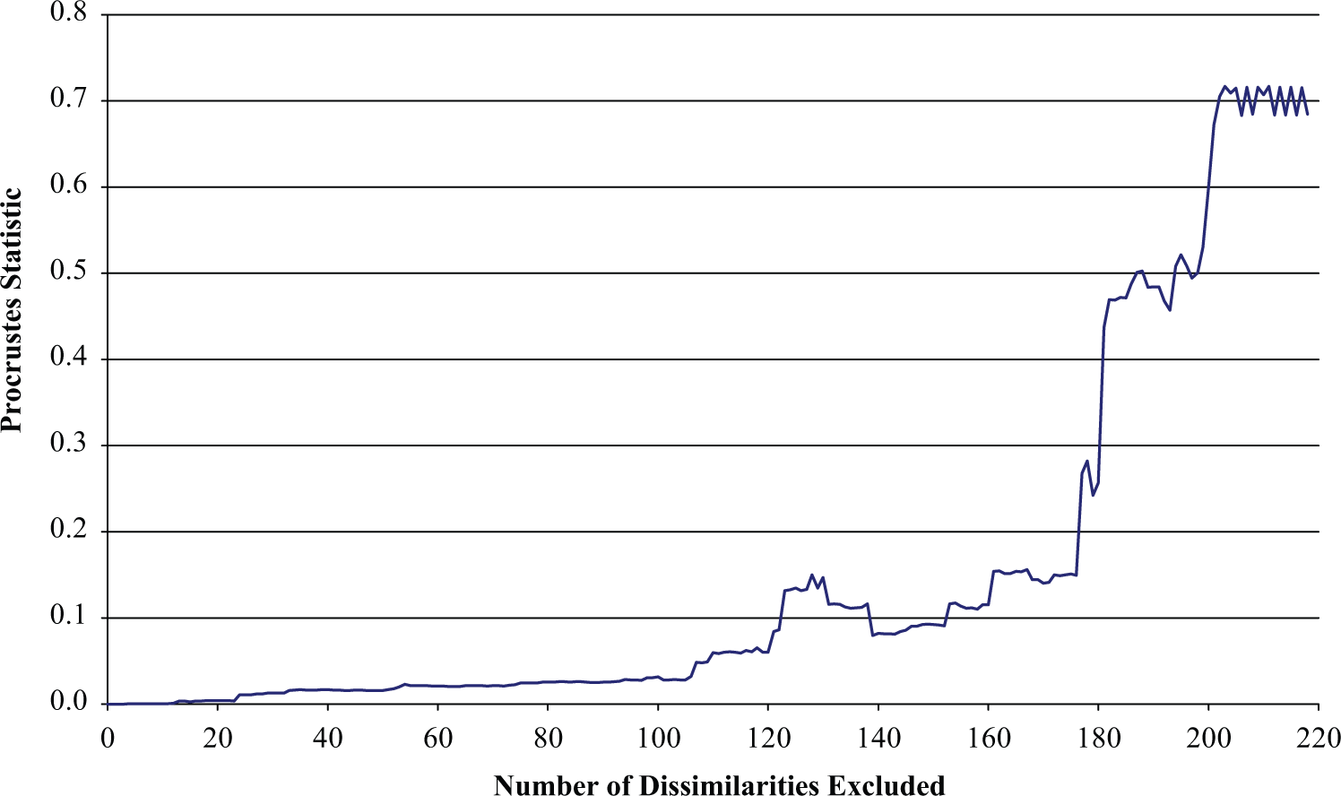
Procrustes statistic with successive dissimilarities excluded

For 23 points, the backbone requires 35 dissimilarities from the original 253 available, so removal of 218 dissimilarities is possible. As expected, as the minimal number of dissimilarities is approached, a perfect fit is attained.

Reduction to the backbone radically affects the solution. However, this approach can work. The procedure may prove effective. A two dimensional vector with random entries, but with the same number of points as in the previous example was generated. Dissimilarities were obtained from this vector and subjected to an identical analysis to that used for the cereal data. The graphs are not produced here because in every case, the stress (mean 6⁻¹⁰) and Procrustes statistic (mean 8⁻³³) were effectively 0. Similar results were obtained when deriving an l dimensional solution to data corresponding to an l dimensional vector. So for “perfect” data, the procedure works extremely well.

A check (in particular have the methods been correctly programmed) using a traditional data set of French cities is explored. This is exactly the same example as that used by Tsogo et al. (2001), who provided the raw dissimilarity data in addition to the true structure (the actual map of the French cities) and the recovered structure (a plot of the coordinates resulting from their procedure).

A Traditional Example

This classic example also provides a cautionary tail; it relates to 11 cities of France and was presented by Tsogo et al. (2001). The inter-city distances were obtained from the French railway company (SNCF). The authors very kindly not only provided the full data set of dissimilarities but also identified the backbone. As a check on the calculation, the latitude/longitude of the towns was obtained. These coordinates will not strictly match the SNCF distances, because the rail distances will not necessarily be the shortest route between cities. Using these coordinates, the dissimilarities retained in the backbone (Tsogo et al., 2001) are indicated in Figure 3.

OPEN IN VIEWER

Figure 3.

The backbone for a traditional problem

The solution of the two options (full solution and the backbone problem) using MDS and LSQ are displayed in Figure 4, with the associated Procrustes statistics in Table 1. Units have been included on the axis in Figure 4, although this is not strictly necessary, because any translation, rotation, and reflection of the configuration of points will give rise to an equivalent solution. For the solutions reported here, 1,000 random starts were used to avoid identifying a local minimum, followed by at most 500 cycles of the algorithm (Kruskal, 1964; Lingoes & Roskam, 1973). As a comparison, the coordinates obtained from Tsogo et al. (2001; Figure 9c) provide the final row/column in Table 1.

OPEN IN VIEWER

Figure 4.

Comparison of the solutions using MDS and LSQ for a traditional problem

OPEN IN VIEWER

Table 1.

Procrustes Comparison of the Solutions Using MDS and LSQ for a Traditional Problem.

	True location	Full LSQ solution	Backbone LSQ solution	Full MDS solution	Backbone MDS solution	Tsogo et al. solution
True location	0	0.0695	0.6406	0.3296	0.5552	0.1286
Full LSQ solution	0.0695	0	0.7414	0.2260	0.6081	0.0774
Backbone LSQ solution	0.6406	0.7414	0	0.6539	0.7523	0.6722
Full MDS solution	0.3296	0.2260	0.6539	0	0.7561	0.3780
Backbone MDS solution	0.5552	0.6081	0.7523	0.7561	0	0.6095
Tsogo et al. solution	0.1287	0.0775	0.6722	0.3780	0.6096	0

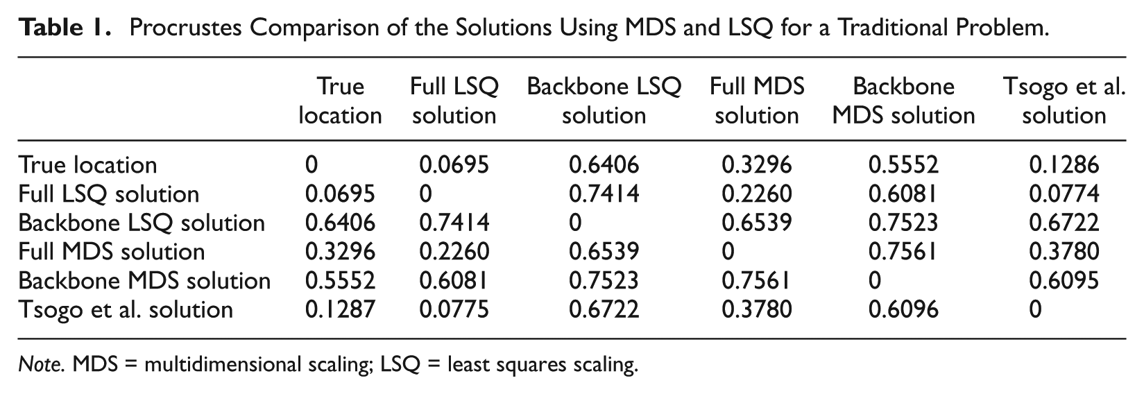
Note. MDS = multidimensional scaling; LSQ = least squares scaling.

As expected, the full set of dissimilarities provide a good fit to the true (geographic) location, which is not the case with the backbone. This is contrary to results previously reported by Tsogo et al. (2001), who, on comparing the true and recovered structure, “concluded that these two structures are visually similar.” Their solution corresponds to the LSQ approach. It is illuminating to report the function values corresponding to the solutions.

The MDS stress from the full solution was 12% and that for the backbone solution was 0%, while that for the Tsogo et al. (2001) was 6%. The LSQ stress from the full solution, that for the backbone solution and that for the Tsogo et al. were all 0%. Hence, they all provide a perfect fit. As pointed out by Tsogo et al., “the minimisation is not a straightforward optimization problem because of the very complex response surface over which the search is carried out.” Therefore, caution must be used; the starting position may greatly affect the solution. It is unclear which starting point was used in the original work. In the LSQ case, there is no criterion to aid in the selection of a specific solution, all providing a perfect fit.

The appearance of the backbone solution is not surprising, given the adjacency matrix of the selected backbone presented in Table 2.

OPEN IN VIEWER

Table 2.

An Adjacency Matrix For the Backbone Problem: Sorted by Cluster.

	Brest	Dijon	Lille	Nice	Rennes	Lyon	Marseille	Toulouse	Grenoble	Paris	Strasbourg
Brest	0	1	1	0	0	1	0	0	0	0	1
Dijon	1	0	0	0	0	0	1	0	1	0	0
Lille	1	0	0	0	0	0	0	0	1	1	0
Nice	0	0	0	0	0	0	1	1	1	0	0
Rennes	0	0	0	0	0	1	0	0	0	1	1
Lyon	1	0	0	0	1	0	0	0	1	1	0
Marseille	0	1	0	1	0	0	0	0	0	0	1
Toulouse	0	0	0	1	0	0	0	0	0	1	1
Grenoble	0	1	1	1	0	1	0	0	0	0	0
Paris	0	0	1	0	1	1	0	1	0	0	0
Strasbourg	1	0	0	0	1	0	1	1	0	0	0

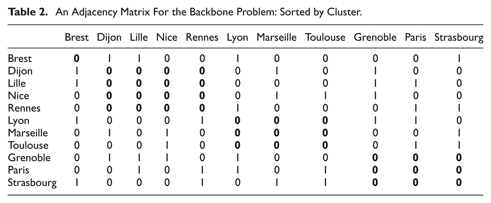
Here, cities connected by a backbone dissimilarity (such as Brest and Dijon) are adjacent and have an entry “1,” all other values being 0. The cities are arranged to reflect the clusters in the backbone solution of Figure 4. The reason for the clustering becomes clear on examining the highlighted diagonal entries. There are no internal dissimilarities defined within the clusters, for instance, linking (Dijon, Lille, Nice, and Rennes). This is less of a problem if LSQ is used (Figure 4 and Table 1).

Uniqueness of the solution is a problem. The binary matrix provides the structure; any permutation of the labels (cities) will suffice. In addition, if, say, three points lay in a straight line, the structure, while rigid, would not be unique. So if they were in an effectively straight line, a reflected reconstruction would produce very little stress but a very poor reconstruction from the visual point. In general, the coordinates of the individual points (and their linearity) are not available in advance and so cannot be used when selecting the backbone.

Contrary to suggestions made elsewhere (Tsogo et al., 2001), the backbone procedure does not necessarily reconstruct a geometrical configuration using minimal information. This has been illustrated by the examples investigated here. However, there is certainly a place for extracting the backbone and analyzing this information. The solution(s) obtained differ from that for the full problem. The backbone appears reliable when using LSQ. It also works well if the data are reliable in accurately reflecting the Euclidean distance between the points. This was illustrated by adopting a random approach to data matching the dimension of the cereal data. Unfortunately, in reality, this situation is unlikely to occur. A perfect (error-free) m dimensional solution, to a set of observed dissimilarities, is unlikely to arise. One constructive suggestion is to use the backbone, with its ease of analysis, to provide a starting point for analysis of the full problem.