An Extension of the DINA Model Using Covariates

Abstract

When students solve problems, their proficiency in a particular subject may influence how well they perform in a similar, but different area of study. For example, studies have shown that science ability may have an effect on the mastery of mathematics skills, which in turn may affect how examinees respond to mathematics items. From this view, it becomes natural to examine the relationship of performance on a particular area of study to the mastery of attributes on a related subject. To examine such an influence, this study proposes a covariate extension to the deterministic input noisy “and” gate (DINA) model by applying a latent class regression framework. The DINA model has been selected for the study as it is known for its parsimony, easy interpretation, and potential extension of the covariate framework to more complex cognitive diagnostic models. In this approach, covariates can be specified to affect items or attributes. Real-world data analysis using the fourth-grade Trends in International Mathematics and Science Study (TIMSS) data showed significant relationships between science ability and attributes in mathematics. Simulation study results showed stable recovery of parameters and latent classes for varying sample sizes. These findings suggest further applications of covariates in a cognitive diagnostic modeling framework that can aid the understanding of how various factors influence mastery of fine-grained attributes.

Keywords

DINA model latent class regression TIMSS

When students solve problems, their proficiency in a particular subject may influence how well they perform in a similar, but different area of study. In particular, it is viewed that mathematics and science have a structural and functional relationship; mathematics can be used as a tool for science, and science can also function as a stimulus for further mathematical discoveries (Li, Shavelson, Kupermintz, & Ruiz-Primo, 2002). Educators have implemented this tradition into the curriculum by teaching the interconnectedness of mathematics and science domains (Halton, 1973). Assessments that require the use of skills from both subjects have been developed, and mathematics items from the Trends in International Mathematics and Science Study (TIMSS) are taken to demonstrate this idea (see Figure 1).

Figure 1.

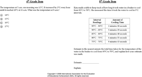
Exemplar mathematics items from the fourth- (Left: M031335) and eighth-grade (Right: M022232) TIMSS.

In Figure 1, two items are presented from two grade levels: fourth and eighth grade. Both items are mathematics items; however, they require basic knowledge in science, in particular the principle of temperature measurement. For the fourth-grade item on the left, examinees are asked to calculate the increase in temperature after 2 hours, assuming that temperature increases by intervals of 2° every hour. In addition to skills in whole numbers, students need to grasp the scientific context used in a Celsius scale to correctly apply the mathematical concepts. A similar idea is demonstrated in the eighth-grade item. In this item, the examinee is asked to estimate the time for the beaker to cool, given the temperature and duration provided in the table. Although this item does not require the sole knowledge of science skills, it does require basic principles of temperature and duration of heat to answer the item correctly. Although the two exemplar items do not infer causal relationships, there is an association in skills that extend beyond one specific subject of study.

From this view, it becomes natural to examine the relationship science ability may have on mathematics skills, which in turn may also affect how examinees respond to mathematics items. Again, the relationship may not necessarily be causal, but the direction and magnitude of association can be valuable information. In fact, the question that may be of value to instructors and researchers is whether features of science are related to specific mathematics skills; conversely, they can also ask whether mathematics ability affects specific attributes in science. This concept extends above and beyond calculating simple correlations of student performance in mathematics and science that is traditionally done in many studies. If the ability and knowledge from one subject area can influence the mastery of skills and concepts in another area, then identifying these specific fine-grained skills can improve not only instruction but also feedback to students that lack such skills. Although previous modes of research have investigated the relationship between mathematics and science education from broad content domains, there has not been a study that examined the effect that knowledge in either subject affects the likelihood of an examinee to master skills or improve solving questions in a different subject.

Cognitive diagnostic models (CDMs) provide an ideal framework for conducting such an analysis as it classifies examinees into attribute profiles that indicate their mastery in fine-grained skills. This study extends the deterministic input noisy “and” gate (DINA; Junker & Sijtsma, 2001) model by including a covariate. In the DINA model, a covariate can be specified at two levels; at the lower level, it can affect how examinees solve items (i.e., response probability), and at the higher level, it can influence the mastery of attributes (i.e., latent classification). That is, the DINA model can be specified to investigate the effect that science ability has on an examinee’s probability of solving mathematics items; it can also be parameterized to examine the influence that science ability has on the mastery of fine-grained mathematics skills.

This study introduces a framework for examining a covariate extension of the DINA model, demonstrated using real-world data from the TIMSS where science proficiency is modeled as a covariate for the mastery of skills required for mathematics items. A simulation study is supplemented to investigate parameter recovery and sensitivity of the model under various specifications of sample sizes, attributes, and its relationship to the covariate. The combination of both real-world data analysis and simulation study will inform researchers on the use of covariates to examine the relationship between factors that influence items and attributes as possible sources of additional diagnostic information. In addition, the results of this study provide a meaningful extension of the DINA model to answer questions of substantive need and also provide implications for more complex and generalized CDMs.

Theoretical Framework

DINA Model

The DINA model requires the identification of skills or attributes needed to answer a question and implements the construction of a Q-matrix (Tatsuoka, 1985). Let Y_ij be examinee i’s response for item j, and $\underline{α} = (α_{1}, α_{2}, …, α_{K})'$ be a vector of K attributes, which indicates the presence or the absence of the attributes. The Q-matrix is a J by K binary matrix that specifies the relationship between the items and the attributes; a value of 1 signals the requirement of the particular attribute, whereas the value of 0 represents that the particular attribute is not necessary.

The DINA model is a conjunctive model, which assumes that all specified attributes are required for an examinee to solve the problem. This is indicated by the binary latent variable, $η_{ij} = Π_{k = 1}^{K} α_{ik}^{q_{jk}}$ , which classifies whether examinee i has mastered all required attributes for item j. The DINA model calculates the probability that examinee i solves item j correctly given the attribute vector η_ij as,

p (Y_{i j} = 1 | η_{i j}) = {(1 - s_{j})}^{η_{i j}} {(g_{j})}^{1 - η_{i j}} .

There are two parameters: the slip and the guessing parameters (Junker & Sijtsma, 2001). Students who possess all the attributes required for an item can slip and incorrectly answer the item, and students who do not possess all the attributes required for an item may guess and correctly answer the item. The DINA model defines the slip parameter as $s_{j} = p (Y_{ij} = 0 | η_{ij} = 1)$ and the guessing parameter as $g_{j} = p (Y_{ij} = 1 | η_{ij} = 0)$ for item j. A reparameterized version of the DINA model from Equation 1 takes the logit function of the DINA model as follows:

logit p (Y_{i j} = 1 | η_{i j}) = f_{j} + d_{j} η_{i j} .

In the reparameterized deterministic input noisy “and” gate model (RDINA; DeCarlo, 2011), the f_j parameter provides the log odds estimates of the guessing parameter, whereas the d_j parameter provides a measure of how well the item can discriminate an examinee with or without the mastery of the attribute. As noted in Junker and Sijtsma (2001), exponentiating the parameters yields the original guessing and slip parameters as follows:

g_{j} = \exp (f_{j}) / [1 + \exp (f_{j})],

s_{j} = 1 - \exp (f_{j} + d_{j}) / [1 + \exp (f_{j} + d_{j})] .

A Covariate Extension to the DINA Model

Various latent class models have incorporated covariates as extensions (Dayton & Macready, 1988; DeCarlo, 2005; van der Heijden, Dessens, & Böckenholt, 1996). In the DINA model, covariates can be specified at two levels: at the lower level, characterized by item parameters, and at the higher level that measures the attributes. Dayton and Macready (1988) introduced the view that covariates can affect the latent class (attribute) probabilities and demonstrated a case using a logistic model. This approach is meaningful in the CDM approach, because this allows an interpretation of covariates that can serve its diagnostic purpose. Treating the DINA model as a latent class model, examinee i’s response probabilities can be modeled as follows (DeCarlo, 2011):

p (Y_{i 1}, Y_{i 2}, …, Y_{i J}) = \sum_{\underline{α}} p (\underline{α}) p (Y_{i 1}, Y_{i 2}, …, Y_{i J} | \underline{α}) = \sum_{\underline{α}} p (\underline{α}) \prod_{j} p (Y_{i j} | \underline{α}) .

Equation 5 indicates that the unconditional response probability is the weighted sum of the conditional response probability across the latent classes (see first two terms of the equation). Applying the basic assumption of independence for the responses given latent classes (Clogg, 1995), the third term can be derived, where the p(Y_ij | $\underline{α}$ ) term is the DINA model from Equation 1. When the constrained assumption of independence for the attribute structure is applied, $p (\underline{α})$ becomes

p (\underline{α}) = \prod_{k} p ({\underline{α}}_{k}) = \prod_{k} \exp (b_{k}) / [1 + \exp (b_{k})] .

As expressed in Equation 6, the model for $p ({\underline{α}}_{k}) = \exp (b_{k}) / [1 + \exp (b_{k})]$ uses an attribute difficulty parameter, b_k. The use of the independence model in the formation of the covariate extension provides a useful comparison with more complex CDMs (von Davier, 2014) that may assume a conditional independence structure, such as the higher order–deterministic input noisy “and” gate model (HO-DINA; de la Torre & Douglas, 2004).

When a discrete or a continuous covariate, $\underline{Z}$ , is introduced into the framework, the equation for the response probability in Equation 5 can be modified as follows:

p (Y_{i 1}, Y_{i 2}, …, Y_{i J} | \underline{Z}) = \sum_{\underline{α}} p (\underline{α} | \underline{Z}) \prod_{j} p (Y_{i j} | \underline{α}, \underline{Z}) .

Equation 7 represents the response probability conditioning on the covariate $\underline{Z}$ that can subsequently be separated into two terms to examine the effect of the covariate on the response probabilities, p(Y_ij | α, Z ), or on the attribute probability, p(α | Z ). Equation 8 shows the term for the covariate affecting the response probability, and Equation 9 shows the term for the covariate affecting the attributes:

logit p (Y_{i j} | \underline{α}, \underline{Z}) = f_{j} + d_{j} η_{i j} + l_{j} \underline{Z},

logit p (α_{k} | \underline{Z}) = b_{k} + h_{k} \underline{Z} .

When the covariate is conditioned on the response probabilities, the covariate can shift the estimate of the guessing and slip parameters. For simplicity, if we assume that Z is a binary covariate, then the presence or the absence of the covariate (i.e., Z = 1 or 0) can influence the guessing and slip rates in the DINA model by a factor of l_j, conditional on the value of the covariate. Equation 10 shows the increase in the guessing parameter for examinees with Z = 1, and Equation 11 shows the decrease in the slip parameter for examinees with Z = 1. For continuous covariates, the parameter l_j indicates changes in the guessing and slip parameters for a unit increase in Z, conditional on the value of the covariate:

g_{j} = \exp (f_{j} + l_{j}) / [1 + \exp (f_{j} + l_{j})],

s_{j} = 1 - \exp (f_{j} + d_{j} + l_{j}) / [1 + \exp (f_{j} + d_{j} + l_{j})] .

When the covariate is conditioned on the attribute probabilities as expressed in Equation 9, it becomes a predictor of the attribute patterns that affect the latent class membership. Similar to the interpretation of the item-level parameter, l_j, the parameter h_k reflects the shift in the attribute difficulty parameter, b_k, when the covariate is present to affect the attribute. When a conditional independence model is assumed, the covariate extension could be added; for example, if a HO-DINA model is used to account for a higher order θ that uses the K attributes as indicators of a latent trait, then Equation 9 will be $logit p (α_{k} | \underline{Z}, θ) = b_{k} + a_{k} θ + h_{k} \underline{Z}$ , where the parameter h_k will affect the attribute difficulty (b_k) and attribute discrimination (a_k) parameters for different levels of Z . As such, estimates of parameters l_j and h_k can infer information about the covariate and its influence on the item and on the attribute, respectively.

Study I: Real-World Data Study

Method

The covariate extension of the DINA model is examined using the 2007 TIMSS fourth-grade data. The TIMSS releases data in block formats that provide about 20 to 30 items per group of examinees (Foy & Olson, 2009). The advantage of using TIMSS to conduct this study is that it is one of the rare international assessments that provides both mathematics and science performance at the item level for the same examinee. The data used for this study consisted of 25 mathematics items from Booklet 4 using combined data (n = 825) from the U.S. national sample and two benchmark states—Massachusetts and Minnesota. A Q-matrix was derived from Lee, Park, and Taylan (2011), which originally had 15 attributes; these attributes were collapsed by related skills in a particular domain to reduce the number of attributes to seven (see Table A1, in the online supplement). The collapsing of the attributes was conducted to resemble topic areas in the TIMSS 2007 framework.

Examinee’s number-correct score from the science assessment (27 items) was used as a covariate. At the fourth-grade level, students were tested on knowledge from physical science, life science, and earth science. In mathematics, three content domains, Number, Geometric Shapes and Measures, and Data Display, were tested. Using the empirical data, three models were fit: (a) RDINA model, (b) RDINA model with the science number-correct score affecting attributes (latent classification), and (c) RDINA model with the science number-correct score affecting items (response probabilities). Model fit indices were calculated using information criteria measures (Akaike information criterion [AIC] and Bayesian information criterion [BIC]) based on the maximum log likelihood estimates (−2LL) to select the best-fitting model.

Estimation was conducted using Latent GOLD 4.5 to fit the RDINA and covariate extensions of the RDINA model. The syntax for fitting the covariate RDINA in Latent GOLD is given in the Appendix (see the online supplement). Both Expectation-Maximization (EM) and Newton–Raphson algorithms were used to obtain maximum likelihood (ML) or posterior mode (PM) estimates. The use of PM estimation avoids boundary problems commonly associated with latent class models (DeCarlo, 2011); this method uses a prior distribution to smooth solutions that are near the boundary of the parameter space. In addition, to avoid problems of local maxima, 100 sets of starting values were used to obtain the global maximum. Finally, to check for local identification, the rank of the Jacobian matrix was examined to be of full rank as specified as a required condition for local identification in latent class regression models (Huang & Bandeen-Roche, 2004).

Results

Model fit

RDINA, RDINA with covariate affecting attributes, and RDINA with covariate affecting items were fit to examine the effect of science ability on mathematics items and on the mastery of mathematics attributes in a CDM framework. Table 1 shows the fit statistics of the three models used for this study.

Table 1.

Fit Statistics.

Model	No. of Parameters	AIC	BIC
RDINA model	57	23,296.54	23,565.32
RDINA models (with science score covariate)
Attribute-level model	64	22,692.78	22,994.56
Item-level model	82	22,317.04	22,703.70

Note. AIC = Akaike information criterion; BIC = Bayesian information criterion; RDINA = reparameterized deterministic input noisy “and” gate.

The first model included no covariate (RDINA), which was fit as a baseline model for comparison. The next RDINA model specified science ability to affect mathematics attributes, which would influence the mastery classification of the seven attributes. The mathematics (M = 14.85, SD = 5.00) and science (M = 17.18, SD = 5.00) number-correct scores had a correlation of .66. Finally, the RDINA model with science ability affecting mathematics items was fit. To select the best-fitting model, results from model fit indices were examined. Both the AIC and BIC indicated that the item-level covariate model fits best with the lowest fit indices. In the RDINA model without covariate, there are 57 parameters from the 50 RDINA item parameters (f_j and d_j) and seven attribute parameters (attribute intercept, b_k). In the models with covariates, additional parameters were estimated. For the attribute-level model, seven additional parameters were estimated for each of the attributes as regression coefficients for the covariate (h_k). For the item-level model, 25 additional regression coefficients for the covariate affecting the items (l_j) were estimated in addition to the original 57 parameters in the RDINA model.

RDINA item parameters

Table 2 presents the f_j and d_j parameters from the RDINA model (the original guessing and slip DINA parameters can be derived by exponentiating the RDINA parameters as indicated in Equations 3 and 4 above). In general, the f_j and d_j parameters were similar between the RDINA and the attribute-level covariate model. Items 1 (Number domain), 6 (Geometric Shapes and Measures domain), and 12 (Data Display domain) had the greatest guessing estimates. For the slip parameter, Items 11 (Geometric Shapes and Measures) and 21 (Number domain) had high estimates, respectively. When compared with the item-level covariate model, the guessing parameters were lower and the slip parameters were higher, indicating a shift in the parameter locations due to the effect of the covariate (l_j) on the RDINA item parameters as expressed in Equations 10 and 11. The average guessing parameter estimates, derived using Equation 3, across the Number domain for the RDINA, RDINA with covariates affecting attributes, and RDINA with covariates affecting items were 0.33, 0.33, and 0.05, respectively; for the Geometric Shapes and Measures domain, they were 0.37, 0.38, and 0.09, respectively; and for the Data Display domain, they were 0.47, 0.48, and 0.10, respectively.

Table 2.

RDINA Item Parameters: f and d Parameters.

Item	Domain	No covariates				Covariate affecting attributes				Covariate affecting items
		f_j		d_j		f_j		d_j		f_j		d_j
1	Number	0.91	(0.12)	1.51	(0.23)	0.89	(0.12)	1.48	(0.22)	−1.56	(0.36)	1.50	(0.25)
2	Number	−2.43	(1.19)	2.58	(1.22)	−2.13	(0.37)	3.01	(0.40)	−5.34	(1.10)	2.06	(0.96)
3	Number	−0.94	(0.13)	1.78	(0.19)	−0.79	(0.12)	1.60	(0.18)	−3.21	(0.38)	2.00	(0.25)
4	Number	0.14	(0.11)	1.93	(0.26)	0.19	(0.10)	2.03	(0.25)	−1.78	(0.32)	1.27	(0.24)
5	Number	−0.42	(0.12)	2.75	(0.24)	−0.44	(0.12)	2.76	(0.24)	−4.30	(0.47)	2.49	(0.28)
6	Geometric Shapes and Measures	1.31	(0.24)	4.60	(3.20)	1.53	(0.19)	7.39	(7.46)	−2.32	(0.94)	6.84	(7.53)
7	Geometric Shapes and Measures	−0.71	(0.22)	1.87	(0.31)	−0.57	(0.17)	2.03	(0.29)	−2.83	(0.45)	1.49	(0.44)
8	Geometric Shapes and Measures	−0.88	(0.12)	1.99	(0.20)	−0.89	(0.12)	1.88	(0.19)	−3.06	(0.36)	1.64	(0.23)
9	Geometric Shapes and Measures	−0.24	(0.26)	2.62	(0.36)	−0.27	(0.27)	2.79	(0.35)	−3.05	(0.65)	2.39	(0.49)
10	Geometric Shapes and Measures	−0.79	(0.27)	1.65	(0.30)	−0.67	(0.25)	1.61	(0.27)	−2.16	(0.43)	1.33	(0.36)
11	Geometric Shapes and Measures	−0.88	(0.12)	0.53	(0.17)	−0.89	(0.12)	0.56	(0.18)	−1.61	(0.29)	0.42	(0.19)
12	Data Display	0.82	(0.11)	1.28	(0.24)	0.81	(0.11)	1.33	(0.24)	−1.01	(0.31)	0.94	(0.24)
13	Data Display	0.49	(0.11)	2.14	(0.27)	0.52	(0.11)	2.05	(0.26)	−2.36	(0.37)	1.71	(0.30)
14	Data Display	−1.08	(0.12)	1.91	(0.22)	−1.02	(0.11)	1.95	(0.20)	−3.01	(0.33)	1.37	(0.22)
15	Number	0.29	(0.11)	2.13	(0.23)	0.23	(0.12)	2.21	(0.23)	−2.34	(0.36)	1.48	(0.23)
16	Number	−1.37	(0.16)	2.98	(0.22)	−1.49	(0.17)	3.04	(0.22)	−5.74	(0.52)	2.45	(0.27)
17	Number	−1.96	(0.17)	1.74	(0.21)	−1.96	(0.17)	1.72	(0.21)	−4.64	(0.43)	1.71	(0.24)
18	Number	−0.41	(0.12)	2.35	(0.21)	−0.41	(0.12)	2.30	(0.21)	−3.43	(0.39)	1.74	(0.23)
19	Data Display	−1.32	(0.14)	2.65	(0.22)	−1.36	(0.14)	2.76	(0.23)	−5.06	(0.47)	2.09	(0.26)
20	Data Display	−0.11	(0.11)	2.07	(0.23)	−0.11	(0.10)	2.19	(0.24)	−1.89	(0.33)	1.66	(0.24)
21	Number	−2.58	(0.23)	1.81	(0.26)	−2.66	(0.24)	1.91	(0.26)	−4.99	(0.48)	1.08	(0.26)
22	Geometric Shapes and Measures	−0.61	(0.18)	0.91	(0.23)	−0.64	(0.15)	1.08	(0.20)	−1.58	(0.31)	0.53	(0.27)
23	Number	−0.74	(0.13)	2.78	(0.22)	−0.81	(0.13)	2.77	(0.21)	−4.45	(0.44)	2.33	(0.24)
24	Geometric Shapes and Measures	−1.62	(0.32)	1.91	(0.34)	−1.54	(0.28)	1.83	(0.30)	−3.10	(0.54)	1.74	(0.46)
25	Data Display	0.42	(0.11)	2.49	(0.33)	0.42	(0.11)	2.57	(0.33)	−3.20	(0.44)	2.29	(0.39)

Note. The values in parentheses represent standard errors. The f_j and d_j parameters can be reparameterized to derive the guessing and slip parameters: guessing = exp(f_j)/[(1 + exp(f_j)] and slip = 1 − {exp(f_j+ d_j)/[(1 + exp(f_j+ d_j)]}. The discrimination index (de la Torre, 2008), δ = 1 − guessing − slip, can be calculated based on the following: {exp(f_j+d_j)/[(1 + exp(f_j+d_j)]} − {exp(f_j)/[(1 + exp(f_j)]}. RDINA = reparameterized deterministic input noisy “and” gate.

For the slip parameter derived using Equation 4, the average estimates across the Number domain for the three models were 0.25, 0.24, and 0.83, respectively; for the Geometric Shapes and Measures domain, they were 0.29, 0.28, and 0.66, respectively; and for the Data Display domain, they were 0.14, 0.14, and 0.71, respectively. As these values indicate, the guessing and slip parameter estimates for the RDINA and covariate model affecting attributes were very close. However, the parameter estimates for the covariate model affecting items were shifted down for the guessing and shifted up for the slip parameters.

Discrimination indices that represent how well an item is able to classify an examinee as having mastered an attribute were calculated for each item, δ = 1 −g−s (de la Torre, 2008). This discrimination index was calculated based on the RDINA using the following form: δ = 1 −g−s = {exp(f_j+d_j)/[(1 + exp(f_j+d_j)]} − {exp(f_j)/[(1 + exp(f_j)]}. For the Number domain, the mean discrimination estimates for RDINA, RDINA with covariates affecting attributes, and RDINA with covariates affecting items were 0.41, 0.42, and 0.12, respectively; for the Geometric Shapes and Measures domain, the mean estimates were 0.35, 0.36, and 0.18, respectively; and for the Data Display domain, the mean estimates were 0.36, 0.37, and 0.30, respectively. These estimates show that the discrimination indices decreased for the covariate model affecting items due to the lower guessing and higher slip parameter estimates; the extent that the slip parameters shifted up was greater than the extent that the guessing parameters shifted down.

Unique parameters from the covariate model affecting attributes

Table 3 shows the regression coefficients (h_k) for the covariate model affecting attributes. Science score affected the response probabilities of all attributes, except Attribute 4 (Lines and Angles), which did not have a significant effect (p = .120). Among the attributes, science score had relatively large effects on Whole Numbers, Location and Movement, and Fractions and Decimals.

Table 3.

Attribute Parameters: Covariate (Science Score).

Attribute	Attribute parameter (h_k)		p value
1. Whole Numbers	0.34	(0.03)	<.001
2. Fractions and Decimals	0.33	(0.05)	<.001
3. Number Sentences, Patterns, and Relationships	0.21	(0.10)	.041
4. Lines and Angles	0.14	(0.09)	.120
5. Two- and Three-Dimensional Shapes	0.23	(0.03)	<.001
6. Location and Movement	0.34	(0.09)	<.001
7. Reading, Interpreting, Organizing, and Representing	0.21	(0.06)	<.001

Note. Values represent regression coefficient (h_k) in the covariate model affecting attributes; values in parentheses represent standard errors.

Unique parameters from the covariate model affecting items

Items 5, 16, and 23 from the Number domain; Items 19 and 25 from the Data Display domain; and Item 6 from the Geometric Shapes and Measures domain had the greatest estimates. On average, the parameter estimates for the Number, Geometric Shapes and Measures, and Data Display domains were 0.17, 0.13, and 0.18, respectively. Estimates of l_j for items ranged between 0.05 and 0.27, and all estimates were p < .01; specific regression coefficients l_j for the covariate model affecting items are presented in Table A2 (see online supplement). The significance of these estimates indicates that science score affected the item response probabilities for all 25 items tested.

Attribute prevalence

Table 4 presents the attribute prevalence of the seven attributes. Attribute prevalence is the latent class size of the seven attributes, α_k (DeCarlo, 2011).

Table 4.

Attribute Prevalence.

Attribute	No covariate		Covariate: Attributes		Covariate: Items
1. Whole Numbers	0.56	(0.02)	0.58	(0.02)	0.58	(0.03)
2. Fractions and Decimals	0.81	(0.06)	0.57	(0.04)	0.82	(0.07)
3. Number Sentences, Patterns, and Relationships	0.98	(0.02)	0.91	(0.06)	0.99	(0.02)
4. Lines and Angles	0.97	(0.04)	0.90	(0.08)	0.93	(0.08)
5. Two- and Three-Dimensional Shapes	0.74	(0.04)	0.73	(0.04)	0.76	(0.06)
6. Location and Movement	0.90	(0.07)	0.74	(0.06)	0.76	(0.10)
7. Reading, Interpreting, Organizing, and Representing	0.85	(0.03)	0.71	(0.05)	0.81	(0.05)

Note. The values in parentheses represent standard errors.

For Attributes 3 (Number Sentences, Patterns, and Relationships) and 4 (Lines and Angles), the attribute prevalence was particularly high, above 0.90; this was consistent across the three models. The attribute prevalence for Attributes 1 (Whole Numbers) and 5 (Two- and Three-Dimensional Shapes) had lower probabilities, but remained consistent. However, for Attributes 2 (Fractions and Decimals), 6 (Location and Movement), and 7 (Reading, Interpreting, Organizing, & Representing), their prevalence was lower for the covariate model affecting attributes. The significance in the regression coefficient for these attributes affected the intercept parameter to decrease the attribute prevalence. However, given the large regression parameter (h_k) for Attribute 1 (Whole Number), there was no change in its prevalence (change from 0.56 to 0.58 between the RDINA model without a covariate and the covariate model affecting the attribute, respectively). The marginal change in prevalence, given the large estimate of h₁ (0.34, p < .001; see Table 3), was partly due to the structure of the Q-matrix for Attribute 1, which was specified in 18 items (see Table A1, online supplement). In comparison, for Attribute 2 with a similar parameter estimate (h₂ = 0.33, p < .001; see Table 3) but specified in only 4 items, the attribute prevalence shifted from 0.81 to 0.57. These results indicate that the effect of h_k on the prevalence of attribute k is affected not only by the covariate but also by the Q-matrix structure, which indicates how frequently the attribute is specified.

Study II: Simulation Study

Method

A simulation study was conducted to examine the parameter recovery of the (a) RDINA, (b) RDINA model with covariate affecting attributes, and (c) RDINA model with covariate affecting items. Four sample sizes of 500, 1,000, 2,000, and 5,000 were used across a specification of five and seven attributes. Data were generated using population (true) values derived from the TIMSS real-world data analyzed in the previous section (see Q-matrix in Table A1, online supplement). For creating the Q-matrix for five attributes, two attributes among the seven attributes were collapsed, based on recommendation from mathematics educators: Attributes 2 (Fractions and Decimals) and 3 (Number Sentences, Patterns, & Relationships) were combined, and Attributes 4 (Lines and Angles) and 5 (Two- and Three-Dimensional Shapes) were combined. The use of TIMSS estimates represents a realistic value of parameters, rather than selecting values defined by the authors. Similar to the real-world data analysis, only one continuous covariate (M = 17.18, SD = 5.00) was used in the simulation study. Depending on the model, the probabilities of the attributes (covariate model affecting attributes) and item responses (covariate model affecting items) were generated while being conditioned on the covariate. Moreover, to examine the effect of incorrect models fit to simulated data, data generated using the RDINA model with covariate affecting attributes were fit using the RDINA and RDINA model with covariate affecting items; similarly, RDINA model with covariate affecting items was generated and fit using RDINA and RDINA model with covariate affecting attributes. Together, these represent a total of 56 conditions (24 conditions fit using the correct model + 32 conditions fit using an incorrect model = 3 models × 4 sample sizes × 2 attribute sizes fit using the correct model + 2 covariate models × 4 sample sizes × 2 attribute sizes × 2 incorrect models).

Data were generated using Stata 12 for 100 replications of the 56 conditions studied in the simulation study. A DOS batch file was created to fit the results in Latent GOLD 4.5. Parameter estimates for the replications were summarized and compared with the population values used to generate data. Three measures of parameter recovery, (a) bias, (b) % bias, and (c) mean squared error (MSE), were calculated for each of the conditions. The specific formulas used for calculating bias, % bias, and MSE are presented as follows, where x is an arbitrary indicator of a parameter, e(x) is the generating (true) parameter value, and ${\hat{e}}_{n} (x)$ is the nth replicate estimate of parameter x among a total of N = 100 replications: $Bias (x) = \frac{1}{N} \sum_{n = 1}^{N} [{\hat{e}}_{n} (x) - e (x)] = \frac{1}{N} \sum_{n = 1}^{N} {\hat{e}}_{n} (x) - e (x)$ , % Bias = |Bias(x)/e(x)| × 100%, $MSE (x) = \frac{1}{N} \sum_{n = 1}^{N} {[{\hat{e}}_{n} (x) - e (x)]}^{2}$ . Proportion correctly classified (P_c; Clogg, 1995; de la Torre & Douglas, 2004) was calculated to examine the accuracy in the recovery of latent classes using the maximum posterior probability for each attribute, and % bias was used to measure deviations in the attribute prevalence, compared with generating values. Similar to the real-world data analysis, both ML and PM estimations were used to avoid boundary estimation problems. In addition, to prevent estimation at the local maxima, 20 sets of starting values were used; local identification was checked by ensuring that the Jacobian matrix was of full rank.

Results

RDINA model

Table 5 presents the bias, % bias, and MSE estimates for the eight conditions studied in this model. Results are summarized by averaging the measures of recovery across the parameters to facilitate the presentation of the findings. Three parameters are presented, with one attribute-level parameter representing the intercept of the attribute (b_k), and the remaining two item-level parameters representing the intercept (f_j) and the coefficient (d_j) of the latent class (η_j). For the RDINA model with five attributes, the parameter estimates had % bias estimates that were all below 4% (except for f_j estimates for sample size of 500). The positive mean biases show that the estimates were overestimated. For this condition, estimates of the item intercepts (f_j) had larger bias. In the RDINA model with seven attributes, % bias was larger, reaching 8.7% for the attribute intercept parameter (b_k). In both five- and seven-attribute RDINA models, when sample size increased, the MSE estimates decreased accordingly.

Table 5.

Recovery of the RDINA, RDINA With Covariate Affecting Attributes, and RDINA With Covariate Affecting Items.

	Sample size for five attributes				Sample size for seven attributes
	500	1,000	2,000	5,000	500	1,000	2,000	5,000
RDINA
b_k
Bias	0.018	0.002	0.006	0.006	0.086	0.050	0.028	0.013
% Bias	2.3%	2.7%	2.2%	1.0%	8.7%	4.5%	2.2%	1.7%
MSE	0.035	0.025	0.014	0.005	0.096	0.059	0.035	0.019
f_j
Bias	0.025	0.012	0.001	0.004	−0.008	0.001	−0.014	−0.005
% Bias	7.3%	3.7%	2.7%	1.8%	7.0%	2.3%	2.2%	1.2%
MSE	0.099	0.060	0.037	0.033	0.084	0.046	0.035	0.016
d_j
Bias	0.015	0.008	0.017	0.009	0.030	0.027	0.042	0.043
% Bias	3.4%	2.1%	1.3%	0.8%	4.2%	1.8%	2.0%	1.4%
MSE	0.214	0.123	0.084	0.052	0.207	0.117	0.100	0.086
RDINA with covariate affecting attributes
h_k
Bias	−0.003	−0.001	0.003	0.000	−0.003	−0.004	0.003	0.001
% Bias	1.9%	0.6%	1.1%	0.6%	5.5%	6.0%	2.4%	1.8%
MSE	0.005	0.003	0.002	0.001	0.009	0.008	0.003	0.001
b_k
Bias	−0.040	−0.019	0.010	−0.004	0.000	−0.016	0.011	0.004
% Bias	2.6%	1.5%	0.6%	0.7%	9.6%	12.7%	7.6%	12.8%
MSE	0.366	0.211	0.107	0.036	0.640	0.519	0.211	0.098
f_j
Bias	−0.016	−0.007	−0.007	−0.005	−0.013	−0.009	−0.006	−0.003
% Bias	4.4%	3.8%	1.5%	2.6%	4.4%	1.9%	2.2%	1.0%
MSE	0.059	0.029	0.014	0.006	0.055	0.029	0.012	0.005
d_j
Bias	−0.031	−0.035	−0.019	−0.004	−0.057	−0.072	−0.063	−0.051
% Bias	2.6%	1.8%	1.1%	0.7%	4.5%	2.4%	1.8%	1.4%
MSE	0.254	0.145	0.082	0.053	0.466	0.313	0.215	0.138
RDINA with covariate affecting items
b_k
Bias	−0.009	−0.008	−0.002	−0.003	0.155	0.094	0.051	0.019
% Bias	3.7%	4.6%	2.4%	1.2%	13.9%	9.5%	5.8%	3.2%
MSE	0.045	0.021	0.009	0.004	0.159	0.086	0.048	0.032
l_j
Bias	0.001	0.000	0.000	0.000	0.002	0.001	0.001	0.000
% Bias	1.7%	1.1%	0.8%	0.6%	2.3%	1.4%	1.0%	0.4%
MSE	0.001	0.000	0.000	0.000	0.001	0.000	0.000	0.000
f_j
Bias	0.029	0.023	−0.001	0.009	−0.017	−0.028	−0.022	−0.011
% Bias	2.9%	2.0%	1.5%	0.9%	2.9%	1.3%	1.2%	0.6%
MSE	0.528	0.231	0.101	0.047	0.445	0.208	0.104	0.047
d_j
Bias	−0.133	−0.108	−0.081	−0.070	−0.040	−0.049	−0.054	−0.050
% Bias	6.0%	4.1%	3.2%	2.1%	8.2%	4.7%	3.3%	2.1%
MSE	0.707	0.431	0.276	0.202	0.655	0.372	0.277	0.183

Note. The parameter b_k is the intercept parameter affecting the attributes. The parameters h_k and l_j are the coefficient parameters of the covariate affecting the attributes and items, respectively. The parameters f_j and d_j are at the item level. RDINA = reparameterized deterministic input noisy “and” gate; MSE = mean squared error.

Moreover, when the sample size was 1,000 or above, the % bias was all below or equal to 4.5%. However, unlike the five-attribute conditions that had the greatest bias in the item intercept parameter (f_j), in the seven-attribute conditions, the greatest bias was in the attribute intercept parameter (b_k).

RDINA model with covariate affecting attributes

In this model, the h_k parameter represents the coefficient estimate for the covariate affecting the attributes. For the five-attribute conditions, the greatest % bias was from the item intercept parameter (f_j). However, for all sample sizes and parameters, the % bias was all below or equal to 4.4%. For the seven-attribute conditions, the intercept of the attribute-level parameter (b_k) showed the greatest % bias, ranging from 7.6% to 12.8% across the sample sizes. At the attribute level, parameter bias was largest for attributes with population values close to the boundaries; the high bias may be attributed to estimation problems. Across both five- and seven-attribute conditions, the item parameters were underestimated as evidence from the negative bias estimates. Moreover, the MSE estimates decreased when sample size increased. Although the five-attribute condition showed consistent recovery of parameters for varying sample sizes, the % bias of the attribute intercept parameter for the seven-attribute condition was more than 10% even with a sample size of 5,000.

RDINA model with covariate affecting items

This model has the most parameters, as additional parameters have to be estimated for each item, leading to three parameters per item. In addition to the parameters in the RDINA model, the coefficients of the covariate affecting items (l_j) are added. For the five-attribute condition, the parameter d_j had the greatest % bias. The recovery of the l_j parameters had the lowest bias. For the seven-attribute conditions, the greatest % bias was from the b_k parameter; even with a sample size of 2,000, the % bias was above 5%. In general, for both five- and seven-attribute conditions, an increase in sample size decreased % bias and MSE. Furthermore, the d_j parameter was underestimated in both models as indicated by the negative bias estimates. Moreover, for the five-attribute condition, a sample size of 1,000 showed % bias estimates to be less than 5%; a larger sample size more than 2,000 was needed for the seven-attribute condition.

Attribute prevalence and classification

Estimates of the maximum posterior probability were used to classify the mastery in each of the five- and seven-attribute conditions. These classifications were used to calculate the % bias of the attribute prevalence and the P_c statistics. Results are summarized in Table A3 (online supplement) for the five- and seven-attribute conditions across four sample sizes and for the three models examined in this study (RDINA, RDINA with covariate affecting attributes, and RDINA with covariate affecting items). Columns indicate the sample sizes for the two attribute conditions, and the rows indicate the % bias and P_c for each attribute of the three models. Overall, the % bias in attribute prevalence was all below or equal to 2.2% even with a sample size of 500 for the five-attribute condition, across the three models; P_c was all above 0.81. For the seven-attribute condition, the % bias was all below or equal to 14.2% for a sample size of 500, with the largest % bias from Attribute 4; P_c was all above or equal to 0.80. Although small differences in % bias and P_c were found between models, the recovery of attribute prevalence was relatively similar across conditions with only minor changes, indicating stability in attribute prevalence and classification.

Fitting simulated data to incorrect models

Data generated using the RDINA covariate extensions (affecting attributes or items) were fit with incorrect models (e.g., RDINA model with covariate affecting attributes fit using the RDINA model or RDINA model affecting items). Model fit indices, P_c, and % bias of parameters (item and attribute) are presented in the online supplement Table A4. Across the four sample sizes (500, 1,000, 2,000, and 5,000) and five- or seven-attribute conditions, both AIC and BIC selected the correct model. Moreover, the correct model had the highest P_c and the lowest % bias in item parameter estimates. Incorrect models had higher AIC and BIC values and lower P_c estimates. The greatest impact of using incorrect models was found in the % bias of item parameters. When data generated using RDINA with covariate affecting attributes were fit using the RDINA with covariate affecting items, % bias was more than 305% for the five-attribute condition and more than 132% for the seven-attribute condition; conversely, for the RDINA model with covariate affecting items fit using the RDINA with covariate affecting attributes, % bias was more than 102% for the five-attribute condition and more than 86% for the seven-attribute condition. In both cases, fitting the covariate models using the simple RDINA without a covariate resulted in the lower % bias than the incorrect covariate model.

Discussion and Conclusion

Researchers have long used broad domain-based scores from large-scale assessments to improve their educational systems. CDMs were developed to provide more targeted information in the form of score profiles that resolve the limitation of classical methods and unidimensional item response theory (IRT) models. Various CDMs have been proposed in the measurement literature. Although most CDMs provide an ideal framework for conducting an analysis to classify examinees into attribute profiles that indicate their mastery in fine-grained skills, this study extends the DINA framework by including a covariate in a reparameterized DINA model.

As described in this study, a covariate in the DINA model can be specified to affect examinees’ response probability at the lower level; it can also be specified to affect the latent classification by influencing the attributes at the higher level. To investigate how the covariate extension of the DINA model can be applied to real-world data, this study examined the effect of science ability (number-correct score on TIMSS science assessment) on an examinee’s probability of solving mathematics items; it was also parameterized to examine the influence that science ability had on the mastery of fine-grained mathematics skills. As indicated in the results, science ability had a significant effect on both items and attributes; students with higher science ability had a greater likelihood of solving mathematics items as well as being classified as having mastery in six of the seven attributes (all attributes except Lines and Angles) specified in the Q-matrix. These findings do not suggest a causal relationship between science scores and mathematics ability; however, the significant association for the attributes can provide additional studies that can lead to meaningful results for applied researchers.

Results from the simulation study showed stability in the model to recover parameters at various sample sizes, type of covariate model, and number of attributes. In particular, the findings from this study indicate that a sample size of 500 may be adequate to use a covariate within a DINA model when there are five attributes. When there are seven attributes, the required sample size may need to increase to 2,000 examinees for the bias in the parameter estimates to be reduced below a 5% level. Although this study investigated only one test length consisting of 25 items, various test lengths, attributes, and attribute specification in the Q-matrix should be studied. Moreover, different types of covariates (e.g., dichotomous or ordinal) as well as mix of continuous and discrete covariates that include demographic or learning characteristics of students should be examined in future simulations and empirical studies. Classification of latent classes and attribute prevalence were relatively similar across different conditions and models examined, indicating stability in attribute profiles in the framework of a covariate extension in the RDINA framework. Covariates can be specified at the item level as well as at the attribute level; this specification can be extended to parameterize covariates at both attribute and item levels (DeCarlo, 2005). Previous work by Templin (2005) indicated that specifying a covariate such as gender that can affect the higher order latent trait, can have different item parameters, leading to uniform differential item functioning (DIF) in the context of CDMs. Using the current covariate model, such uniform DIF studies can be studied, by examining estimates of parameters when covariates are specified at the item level.

The covariate extension in this article was conducted in the framework of the RDINA model, which used an independence model for the attribute specification. It is noted that the CDM specification is independent of the attribute specification; that is, CDMs can be used in conjunction with any attribute specification, such as saturated, independence, or conditional independence. While a saturated attribute structure that has no constraints represents the most general model for the attribute distribution, this study examined the use of constrained attribute specifications (independence and conditional independence). As such, comparisons of constrained and unconstrained attribute specifications, in the context of covariate extensions in CDMs, may need to be examined in future studies. In that manner, this study provides a basis for comparison and extensions to a wider array of more complex and generalized CDM frameworks in the literature, such as the generalized DINA model (de la Torre, 2011), general diagnostic model (von Davier, 2014), and the loglinear CDM (Henson, Templin, & Wilse, 2009). In addition to applying a covariate in a DINA model, this study provided an ideal demonstration of the TIMSS data to examine features of mathematics and science education and their consequence on international assessments. In the fields of medicine and public health where competency-based learning is emphasized, covariate extensions of CDMs can lead to understanding the interconnectedness between fine-grained constructs. This framework allows meaningful interpretations of the covariate to provide feedback to instructors and examinees and adds to the diagnostic utility of the model, which are central to CDMs.

Footnotes

Declaration of Conflicting Interests

The author(s) declared no potential conflicts of interest with respect to the research, authorship, and/or publication of this article.

Funding

The author(s) received no financial support for the research, authorship, and/or publication of this article.

Supplemental Material

The online data supplements are available at

References

Clogg

C. C.

(1995). Latent class models. In Arminger

Clogg

C. C.

Sobel

M. E.

(Eds.), Handbook of statistical modeling for the social and behavioral sciences (pp. 311-359). New York, NY: Plenum Press.

Dayton

C. M.

Macready

G. B.

(1988). A latent class covariate model with applications to criterion-referenced testing. In Langeheine

Rost

(Eds.), Latent trait and latent class models (pp.129-143). New York, NY: Plenum Press.

DeCarlo

L. T.

(2005). On the use of covariates in a latent class signal detection model for essay grading. Unpublished manuscript.

DeCarlo

L. T.

(2011). On the analysis of fraction subtraction data: The DINA model, classification, latent class sizes, and the Q-matrix. Applied Psychological Measurement, 35, 80-26.

de la Torre

(2008). An empirically-based method of Q-matrix validation for the DINA model: Development and applications. Journal of Educational Measurement, 45, 343-362.

de la Torre

(2011). The generalized DINA model framework. Psychometrika, 76, 179-199.

de la Torre

Douglas

J. A.

(2004). Higher-order latent trait models for cognitive diagnosis. Psychometrika, 69, 333-353.

Formann

A. K.

(1992). Linear logistic latent class analysis for polytomous data. Journal of the American Statistical Association, 87, 476-486.

Foy

Olson

J. F.

(2009). TIMSS 2007 user guide for the international database. Chestnut Hill, MA: International Association for the Evaluation of Educational Achievement.

10.

Halton

(1973). Thematic origins of scientific thought: Kepler to Einstein. Cambridge, MA: Harvard University Press.

11.

Henson

Templin

Wilse

(2009). Defining a family of cognitive diagnosis models using log-linear models with latent variables. Psychometrika, 74, 191-210.

12.

Huang

G. H.

Bandeen-Roche

(2004). Building an identifiable latent class model with covariate effects on underlying and measured variables. Psychometrika, 69, 5-32.

13.

Junker

B. W.

Sijtsma

(2001). Cognitive assessment models with few assumptions, and connections with nonparametric item response theory. Applied Psychological Measurement, 25, 258-272.

14.

Lee.

Y.-S.

Park

Y. S.

Taylan

(2011). A cognitive diagnostic modeling of attribute mastery in Massachusetts, Minnesota, and the US national sample using the TIMSS 2007. International Journal of Testing, 11, 144-177.

15.

Shavelson

R. J.

Kupermintz

Ruiz-Primo

M. A.

(2002). On the relationship between mathematics and science achievement in the United States. In Robitaille

D. F.

Beaton

A. E.

(Eds.), Secondary analysis of the TIMSS data (pp. 233-249). Norwell, MA: Kluwer Academic Publisher.

16.

Tatsuoka

K. K.

(1985). A probabilistic model for diagnosing misconceptions in the pattern classification approach. Journal of Educational Statistics, 12, 55-73.

17.

Templin

(2005). Generalized linear mixed proficiency models for cognitive diagnosis (Unpublished doctoral dissertation). University of Illinois at Urbana-Champagne.

18.

van der Heijden

P. G. M.

Dessens

Böckenholt

(1996). Estimating the concomitant variable latent class model with the EM algorithm. Journal of Educational and Behavioral Statistics, 21, 215-229.

19.

von Davier

(2014). The DINA model as a constrained general diagnostic model: Two variants of a model equivalency. British Journal of Mathematical and Statistical Psychology, 67, 49-71. doi:10.1111/bmsp.12003