Assessing Item-Level Fit for the DINA Model

Abstract

This research focuses on developing item-level fit checking procedures in the context of diagnostic classification models (DCMs), and more specifically for the “Deterministic Input; Noisy ‘And’ gate” (DINA) model. Although there is a growing body of literature discussing model fit checking methods for DCM, the item-level fit analysis is not adequately discussed in literature. This study intends to take an initiative to fill in this gap. Two approaches are proposed, one stems from classical goodness-of-fit test statistics coupled with the Expectation-Maximization algorithm for model estimation, and the other is the posterior predictive model checking (PPMC) method coupled with the Markov chain Monte Carlo estimation. For both approaches, the chi-square statistic and a power-divergence index are considered, along with Stone’s method for considering uncertainty in latent attribute estimation. A simulation study with varying manipulated factors is carried out. Results show that both approaches are promising if Stone’s method is imposed, but the classical goodness-of-fit approach has a much higher detection rate (i.e., proportion of misfit items that are correctly detected) than the PPMC method.

Keywords

DINA model chi-square index power-divergence index posterior predictive model checking false positive rate correct detection rate

Cognitive diagnosis has recently gained prominence in educational and psychological assessment, psychiatric evaluation, and many other disciplines (Rupp, Templin, & Henson, 2010). In cognitive diagnosis, one attempts to identify the tasks, subtasks, cognitive processes, and/or skills involved in responding to items on an assessment. Each task or skill is generally referred to as an attribute. For example, the attributes of a math test might include converting mixed numbers to improper fractions, finding a common denominator, or multiplying fractions.

The main objective of cognitive diagnosis is to discover the participants’ latent profiles (e.g., mastery of skills, presence of disease or disorders) based on their responses to item questions (e.g., answers to exam problems, occurrence of symptoms) and the item information (e.g., item parameters, item-attribute relationship).

Psychometric models designed for cognitive diagnosis are divided into two general camps: continuous latent trait models and latent class models. Latent trait models, such as item response theory (IRT), posit that each examinee can be represented as a point in a K-dimensional space, where K denotes the number of dimensions underlying a series of test items (Reckase, 2009; Wang & Nydick, 2015). Latent class models, such as diagnostic classification models (DCMs), assume that the latent space consists of a constellation of 0-1 discrete cognitive states (denoted by α). Within this framework, each participant is thus provided with a profile detailing the skills (also called “attributes”) that he or she masters. For example, psychiatrists identify patients’ presence or absence of disorders based on their symptoms through their responses to diagnostic questions; teachers learn students’ mastery of different skills based on their answers to exam questions. In doing so, DCM has been shown to potentially support fine-grained diagnosis that can be used for developing targeted interventions (Rupp et al., 2010; Wang, Chang, & Huebner, 2011).

A number of DCMs have been proposed in the literature. One of the earliest, and probably the simplest DCM is the “Deterministic Input; Noisy ‘And’ gate” (DINA) model (Haertel, 1989; Junker & Sijtsma, 2001). The DINA model assumes that, in principle, an examinee must have mastered every attribute associated with a particular item to respond correctly to that item. This model has been studied extensively not only in method-dominant research (e.g., de la Torre & Douglas, 2004; J. Liu, Xu, & Ying, 2012; Wang, 2013), but also in a few applications. For instance, the DINA model is fitted to middle school students’ solutions of mixed-number subtraction problems by different researchers (also known as the fraction-subtraction data hereafter; de la Torre & Douglas, 2004; Sinharay, 2006; Sinharay & Almond, 2007), and more pronouncedly, it guides the large-scale pilot cognitive diagnostic assessment project in China. The assessment project is designed to measure Level 2¹ English proficiency for Grade 6 students (H. Liu, You, Wang, Ding, & Chang, 2014). All stages of this project, from item writing to test assembly, are executed closely conforming to the DINA model.

Like any model-based assessment, one critical step toward implementing the model is to check model-data fit, that is, the agreement between model predictions and observed data. When a model does not fit the data, the validity of using estimated parameters for inference may be compromised. In DCM, the source of misfit could come from the attribute structure, the type of models, the item–attribute relationship matrix (named as Q matrix), or the test-taking behaviors. The assessment of the degree of misfit can take different foci of model fit, item fit, and response fit (or person fit; Cui & Leighton, 2009).

Relative model fit has typically been evaluated using conventional information-based indices (e.g., de la Torre & Douglas, 2008; Rupp et al., 2010; Sinharay & Almond, 2007) such as the Akaike’s information criterion (Akaike, 1974), the Bayesian information criterion (Schwarz, 1978), and the deviance information criterion (Spiegelhalter, Best, Carlin, & Van Der Linde, 2002). Absolute model fit is gauged by a variety of discrepancy-based statistics. An incomplete list includes residuals between observed and model predicted correlations, log-odds ratios of item pairs, proportion of correct individual items (de la Torre & Douglas, 2008; Sinharay & Almond, 2007), model-level chi-square and G² statistics (Rupp et al., 2010), item-level mean absolute difference (MAD), and item-level root mean square error of approximation (RMSEA; Kunina-Habenicht, Rupp, & Wilhelm, 2012). Person fit is checked by either a generalized likelihood ratio test (Y. Liu, Douglas, & Henson, 2009) or the hierarchy consistency index (Cui & Leighton, 2009).

Only a few studies have ever looked into item-level fit analysis (Kunina-Habenicht, Rupp, & Wilhelm, 2012; Oliveri & von Davier, 2011; Sinharay & Almond, 2007). Item-fit analysis describes model-data fit for every item by comparing model predictions and actual responses via a certain discrepancy measure. Item-fit analysis helps identify aberrant items, the deletion or revision of which will improve overall model-data fit for the entire test. Whereas a large body of research exists on item fit for unidimensional and multidimensional IRT models, corresponding research for DCMs is very limited. Sinharay and Almond (2007) presented a case study in which they use chi-square statistics and a Bayesian residual plot to evaluate item fit using a real data set; however, they do not provide any simulation results to evaluate the performance of the fit statistics. von Davier (2008) applied the general diagnostic model (GDM) to the language testing data and he uses mdltm software that provides item-fit information, yet limited details are provided. Oliveri and von Davier (2011) used item-level RMSEA to evaluate item-level fit when fitting the GDM to the PISA (Programme for International Student Assessment) data. In particular, they treated RMSEA as a diagnostic index and compared it with a cut-off value of 0.1. Items with RMSEA > 0.1 are considered poor-fit. Kunina-Habenicht et al. (2012) presented a thorough simulation study showing the Type I error rate and power of two item-fit indices—MAD and RMSEA. Both of the indices rely on the point estimate of examinees’ latent profiles (denoted as α hereafter), which is a multidimensional, binary vector indicating the mastery status of an examinee on all attributes measured by a test. It is subject to potentially large measurement errors for short tests. This study systemically explores the procedures for several item-level fit statistics with Stone’s (2000) method for adjusting for measurement errors in α, using the deterministic input noisy-and-gate model (DINA; Junker & Sijtsma, 2001) as an illustration. This study, therefore, complemented the existing account of item-fit checking methods in the realm of DCMs. The DINA model is chosen because it is one of the earliest, simplest, and most widely used DCMs in practice (e.g., de la Torre, 2009). As the article unfolds below, it will be clear that the proposed approaches as well as the discrepancy measures are not dependent on any specific parameterizations, and thus they can be applied to any DCMs.

Almost all item-fit indices are built upon the discrepancy between the observed and the model predicted responses, with larger discrepancy indicating poorer fit. To compute model prediction, the model parameters need to be properly estimated. The DINA model, and many existing DCMs, can be estimated via either the maximum likelihood procedure (more specifically, the Expectation-Maximization [EM] algorithm) or the Bayesian procedure (i.e., the Markov chain Monte Carlo [MCMC] algorithm; de la Torre, 2009). Depending on the specific model estimation procedure that is used, the resulting item-fit statistics and their sampling distributions need to be carefully scrutinized. It is, therefore, the contribution of the study to explore the performances of two item discrepancy indices coupled with both the EM and the MCMC estimation procedures.

The rest of the article is organized as follows. First, the authors briefly review the DCMs with a special focus on the DINA model and the type of misfit they plan to elaborate upon. Then, they present two item-level discrepancy indices and the procedures of using them with the EM and the MCMC estimation methods. The authors next present a simulation study designed to evaluate whether the proposed methods can correctly identify misfitting items. They finally detail results of the simulation study, explore their methods for item-fit analysis in a real data set, and discuss implications and future studies.

Method

DCMs

The available DCMs are typically divided into conjunctive and disjunctive models. Conjunctive models require that a participant possesses all attributes comprising an item to have a high probability of correctly responding to or endorsing that item. A short list of conjunctive models includes the DINA model, the noisy input deterministic-and-gate model (NIDA; Maris, 1999), and the fusion model (Roussos, DiBello, et al., 2007; Roussos, Templin, & Henson, 2007). Disjunctive models, however, require examinees to possess at least one of the attributes composing an item to have a high probability of correctly responding to that item, including the deterministic noisy-or-gate (DINO) model and noisy input deterministic-or-gate (NIDO) model. Despite the diversity of available parametric models and the existence of non-parametric techniques, there has been a trend toward unifying DCMs within a global modeling framework or family. The three most widely discussed families are the log-linear cognitive diagnostic model family (Henson, Templin, & Willse, 2009), the generalized DINA model family (de la Torre, 2011), and the GDM family (von Davier, 2008). Central to all these models is the Q matrix, representing a priori specified relationships between the attributes and items. Each element, q_jk, in the Q matrix indicates whether item j measures attribute k. If attribute k is measured by item j, q_jk = 1; otherwise, q_jk = 0.

Because the DINA model is a relatively simple conjunctive model that has received the greatest attention in the past decade, the authors focus on the DINA model throughout the article. Let $α_{i} = (α_{i 1}, α_{i 2}, \dots, α_{i K})$ denote the ith examinee’s mastery profile, with α_ik = 1 if examinee i has mastered attribute k, and 0 otherwise, and i = 1, . . . N, where N denotes examinee sample size. K denotes the total number of latent attributes that are measured by a test. Define η_ij as $η_{i j} = Π_{k = 1}^{K} α_{i j}^{q_{j k}},$ which indicates whether examinee i has mastered all the required attributes for item j to answer it correctly (the “deterministic” feature of the model). The item response function posited by the DINA model for examinee i and item j is given by

P (X_{i j} = 1 | α_{i}) = {(1 - s_{j})}^{η_{i j}} g_{j}^{1 - η_{i j}},

(1)

where s_j is the slipping parameter (i.e., the probability of an incorrect response given an examinee with all the required attributes for solving an item) and g_j is the guessing parameter for item j. Both parameters reflect the “noisy” feature of the model.

In cognitive diagnosis, Q matrix is typically constructed by subject matter experts and test developers, but, in practice, the development of the Q matrix using these means has proven to be quite time-consuming and costly (Roussos, DiBello, et al., 2007). Moreover, pre-specified Q matrix by content experts is usually subjective and may not be accurate. The misspecification of the Q matrix could possibly lead to severe lack of fit and seriously inaccurate inferences on the latent attribute profiles (Rupp & Templin, 2008). To overcome this challenge and to provide a data-driven alternative, de la Torre (2008) and J. Liu et al. (2012) recently proposed to estimate, rather than construct subjectively, the Q matrix directly from the observed response patterns using statistical methods. Even so, an empirical investigation of the plausibility of a postulated Q matrix is still necessary when evaluating the fit of DCMs to actual response data (Kunina-Habenicht et al., 2012).

Model misspecification is another potential source of model-data misfit, and it refers to incorrect parameterization of the psychometric component of the modeling process (Chen, Torre, & Zhang, 2013). As alluded to earlier in this section, different attributes interact through either a conjunctive, or a disjunctive rule, to produce an answer to an item. As a result, researchers need to formalize their conceptualization of the hypothesized cognitive processes involved in each item when choosing an appropriate DCM parameterization. Failure to correctly identify the parameterization will, in theory, yield biased parameter estimates and invalid inference. The item-fit analysis methods that are introduced in the subsequent sections are expected to capture those items with misspecified parameterization.

Because almost all DCMs tend to involve a vector of binary latent traits (i.e., α), as opposed to the vector of continuous latent traits in multidimensional IRT models (Hong, Wang, Lim, & Douglas, 2015; Wang & Nydick, 2015), another possible form of misspecification in DCM is thus the misspecification of α. When the psychological constructs represented by the latent variables are generally understood as broadly defined abilities, such as math ability, it may be unrealistic to model the latent variable as binary, or even discrete. In that case, a continuous ability variable may make more sense (Hong et al., 2015). Misspecifying certain elements in α may result in model or item misfit.

Item-fit analysis procedures

The principal idea of item-fit analysis is to classify the examinees into several ability groups and calculate the average discrepancy between the observed and the expected responses pertaining to each ability group. Large discrepancy usually signals a misfitting item. A slew of indices emanating from non-parametric and parametric frameworks within IRT has been proposed for item fit (Orlando & Thissen, 2000) in the second half of the last century and has recently been adapted to the context of DCM (e.g., Sinharay & Almond, 2007). In this section, a list of item-fit analysis procedures will be introduced.

Classical goodness-of-fit statistics

Assume the DINA model is estimated using the EM algorithm (de la Torre, 2009), and the estimated slipping and guessing parameters are denoted by ${\hat{s}}_{j}$ and ${\hat{g}}_{j}$ , respectively, for $j = 1, \dots, J$ . Suppose the test measures K attributes, then there are maximally 2^K possible binary vectors, $α_{l}, l = 1, 2, \dots, 2^{K}$ , in theory. Suppose there are N examinees in the sample, each examinee has an estimated ${\hat{α}}_{i}$ . Because ${\hat{α}}_{i}$ can take on any one of the 2^K possible patterns, then based on ${\hat{α}}_{i}$ , examinees naturally form 2^K distinctive ability groups, also known as equivalent classes (Sinharay & Almond, 2007). Notice that 2^K is the maximum number of equivalent classes that can be formed for a test measuring K attributes, it is possible that the actual number of equivalent classes can be smaller, if some attribute patterns are impossible. This is true when certain attributes are prerequisite of the others, displaying a hierarchical structure (Sinharay & Almond, 2007). Let N_l denote the “observed”² number of examinees in the lth equivalent class (i.e., ${\hat{α}}_{i} = α_{l}$ ). For each item j, let O_lj be the observed number of examinees with attribute pattern α_l (for equivalent class l) who answer item j correctly. It is obtained by counting the number of examinees, out of N_l, whose ${\hat{α}}_{i} = α_{l}$ and X_ij = 1. Let E_lj be the expected number correct for item j and equivalence class l using the DINA model, which is computed as E_lj = N_lp_lj, where p_lj is computed from Equation 1 based on the estimated item parameters.

Appropriate discrepancy measure needs to be selected to quantify the difference between E_lj and O_lj. Following the status quo from IRT fit analysis, one of the most widely used discrepancy measures is Yen’s (1981)Q₁ statistic, which takes the form of

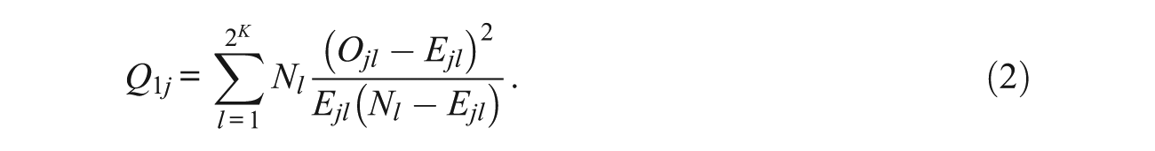
Q_{1 j} = \sum_{l = 1}^{2^{K}} N_{l} \frac{{(O_{j l} - E_{j l})}^{2}}{E_{j l} (N_{l} - E_{j l})} .

(2)

As shown in Equation 2, the Q₁ statistic is algebraically equivalent to the chi-square goodness-of-fit statistic in typical categorical data analysis with two categories (Sinharay & Almond, 2007). This statistic has been studied by many researchers, such as Sinharay (2006) with Bayesian networks (see Equation 6 of his paper), or Toribio and Albert (2011) with unidimensional IRT models.

Yen (1981) showed that in IRT modeling, when the model fits the data, Q₁ is distributed as approximately chi-square with 2^K−mdf, where m is the number of item parameters.³ This df takes into account the estimated item parameters in constructing the expected frequency E_lj, but it does not adjust for the estimation of person parameters. Moreover, when the number of examinees in certain equivalent classes is few, yielding sparse data, the sampling distribution of Q₁ might not be well approximated by a chi-square distribution.

Another widely used discrepancy measure is a likelihood ratio G² statistic (McKinley & Mills, 1985). Both the likelihood ratio and chi-square statistics are widely used in IRT-based item-fit analysis (Levy, Mislevy, & Sinharay, 2009; Orlando & Thissen, 2000) and latent class model diagnosis (Collins, Fidler, Wugalter, & Long, 1993). Moreover, they both can be viewed as a member of the power-divergence (PD) family (Read & Cressie, 1988). This family consists of a group of indices that take the following form, differing only by the parameter λ:

\frac{2}{λ (λ + 1)} \sum_{l = 1}^{T} C_{l} [{(\frac{C_{l}}{E_{l}})}^{λ} - 1],

(3)

where T is the number of groups, C_l is the observed counts in group l, and E_l is the expected counts in group l. Chi-square statistic is the case when λ = 1 and G² is the limit as $λ \to 0$ . However, λ can take on any value. In an extensive study by Read and Cressie (1988), they concluded, not surprisingly, that different values of λ worked best under different conditions. They also find λ = 2/3 as “a good compromise” that is robust in many settings. Thus, the authors applied λ = 2/3 and extend this index to the DCM context, which takes the following form:

P D_{j} = \frac{9}{5} \sum_{l = 1}^{2^{K}} [O_{j l} {(\frac{O_{j l}}{E_{j l}})}^{\frac{2}{3}} + (N_{l} - O_{j l}) {(\frac{N_{l} - O_{j l}}{N_{l} - E_{j l}})}^{\frac{2}{3}} - N_{l}] .

(4)

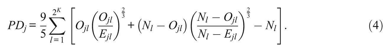
The sampling distribution of the PD index is also approximately a chi-square distribution with $2^{K} - m$ df, with m = 2 for the DINA model. Again this approximation should be used with caution when the data are sparse. An item is flagged as a misfitting item if the p value is lower than a significance level.

Stone’s method

Notice that all current discrepancy measures defined in Equations 2 to 4 rely on ${\hat{α}}_{i}$ for latent class assignment in computing N_l, therefore, the accuracy of ${\hat{α}}_{i}$ will affect the classification of examinees and subsequently, the calculation of discrepancy measures. Classification errors occur when an examinee who should be assigned to a particular ability subgroup is erroneously assigned to a different subgroup. This is particularly likely in tests that are shorter in length and with low informative items. To take the uncertainty of ${\hat{α}}_{i}$ into consideration, rather than using a point estimate of ${\hat{α}}_{i}$ for class assignment, the authors propose to use the posterior probability of ${\hat{α}}_{i}$ . This idea was proposed by Stone (2000) in the context of item-fit analysis in unidimensional IRT models. To implement this idea, the observed counts, O_jl in Equations 3 to 5, are replaced by the “pseudo-counts” (r_jl) of the number of examinees in subgroup l answering item j correctly

r_{j l} = \sum_{i = 1}^{N} x_{i j} p (α_{l} | x_{i}),

(5)

where x_ij denotes the response of the ith examinee to item j; $p (α_{l} | x_{i}) = p (x_{i} | α_{l}) p (α_{l}) / \sum_{l = 1}^{2^{K}} p (x_{i} | α_{l}) p (α_{l})$ is the posterior probability, where $p (α_{l})$ is the prior and $x_{i}$ is the response vector of the ith examinee. N_l and E_lj are also redefined as $N_{l}^{*} = \sum_{i = 1}^{N} p (α_{l} | x_{i})$ and $E_{l j}^{*} = N_{l}^{*} p_{l j}$ , respectively. The two discrepancy indices are denoted as $Q_{1 j}^{*}$ and ${P D}_{j}^{*}$ with Stone’s method.

Because all equivalent classes are not independent due to the fact that each examinee can be assigned to multiple groups with corresponding probabilities, the chi-square distribution is no longer a good approximation to the sampling distribution of the discrepancy measures. Instead, a Monte Carlo resampling technique can be used to construct an empirical null sampling distribution for inference (Stone, 2000).

The resampling procedure involved (a) simulating item response data using the DINA model with item parameters fixed at their estimated values (obtained by calibrating the observed response matrix via the EM algorithm), Q matrix used for model estimation, and randomly sampling αs from its posterior distribution; (b) calibrating the simulated responses using the EM algorithm; and (c) calculating the discrepancy measures in Equations 3 and 4 with Stone’s method of class assignment, using the item parameter estimates from Step b. Steps a to c were repeated 1,000 times to obtain sampling distributions for $Q_{1 j}^{*}$ and ${P D}_{j}^{*}$ . In so doing, the uncertainty in both item and ability parameters was considered in generating the empirical null sampling distribution. For the DINA model, the EM algorithm only takes a few iterations to converge, so the resampling procedure is indeed fast. The observed discrepancy is therefore compared with the empirical null sampling distribution, and the p value is obtained accordingly. If the p value is smaller than the significance level, the null hypothesis is rejected, implying that the item does not fit the data.

Posterior predictive model checking (PPMC)

In addition to the classical goodness-of-fit approach that estimates model parameters first and computes discrepancy measures second, an alternative model checking approach, namely, the PPMC method (Levy et al., 2009; Sinharay, 2006; Toribio & Albert, 2011), has been developed in recent years. The primary idea of PPMC is to compare the test statistics (such as discrepancy measures) from the observed data with the test statistics from the simulated data. The simulated data are obtained via draws of parameter values from the posterior distribution (Meng, 1994), avoiding statistical assumptions about the distributions of the test statistics (Muthén & Asparouhov, 2012). Analytic solutions to the posterior distribution and the posterior predictive distribution of the model parameters are intractable for the DINA model. Instead a MCMC (de la Torre, 2009; Templin, Henson, Templin, & Roussos, 2008) estimation routine forms a good basis to carry out the PPMC method by obtaining M simulated draws from the posterior distribution. In fact, PPMC is often used along with the MCMC estimation algorithm as a Bayesian model checking tool (Meng, 1994). MCMC procedures have been widely used in the DINA model estimation and proven reliable and accurate in simulation settings (e.g., Henson, 2008).

For the ease of exposition, let ω denote the set of parameters (including the item and person parameters); let x denote the observed data (i.e., response matrix in this study’s case). The PPMC method consists of the following steps: (a) drawing M simulated parameters $ω^{1}, ω^{2}, \dots ω^{M}$ from the posterior distribution $p (ω | x)$ , and such parameters are obtained directly from the post burn-in iterations from the MCMC algorithm (M was chosen to be 7,000 in this simulation study below); (b) simulating model-based replicated data, $x^{r e p, m}$ , of the same sample size as the observed data, from the distribution $p (x | ω^{m})$ for m = 1, 2, . . . M; (c) computing the predictive discrepancies $D (x^{r e p, m}, ω^{m})$ and comparing them against the realized discrepancies from the observed data $D (x, ω^{m})$ . The discrepancy measure can be either $Q_{1 j}$ (Sinharay, 2006; Toribio & Albert, 2011) and $P D_{j}$ , or $Q_{1 j}^{*}$ and ${P D}_{j}^{*}$ with Stone’s method.

A quantitative measure of lack-of-fit in the PPMC method is calculated as

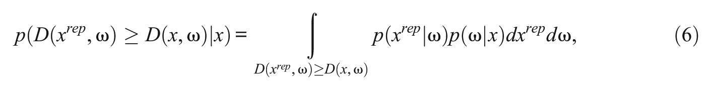
p (D (x^{r e p}, ω) \geq D (x, ω) | x) = \int_{D (x^{r e p}, ω) \geq D (x, ω)} p (x^{r e p} | ω) p (ω | x) d x^{r e p} d ω,

(6)

which is a tail-area probability also named as the PPP value (i.e., posterior predictive p value). Usually, PPP values close to .5 indicate that the realized discrepancies fall in the middle of the distribution of discrepancy measures based on the posterior predictive distribution and are indicative of adequate model-data fit. PPP values near 0 or 1 indicate that the observed discrepancy falls far out in the upper or lower tail of the distribution, implying that the model is under-predicting or over-predicting the quantity of interest (Levy et al., 2009). With the chi-square type of discrepancy measures defined in Equations 3 to 5, the authors sought for PPP values smaller than .05 (for a significance level of .05) in identifying misfitting items, because they were interested in the upper tail area where the observed discrepancy is large.

There are several advantages of the PPMC method. First, the uncertainty in the parameter estimates from the model calibration is taken into account in the computation of the empirical posterior predictive distribution. This is especially beneficial for short tests and small sample size, when both item and person parameter estimates are prone to large measurement errors. Second, this method requires no additional assumptions or regularity conditions (such as zero counts), thus PPMC is valid even when the sample size is too small to warrant the use of asymptotic sampling distributions. Third, it is a general approach and can be applied to any statistical models. Even armed with the prominent advantages, the PPMC method is also open to criticism, mainly because the PPP values are not uniformly distributed (Robins, van der Vaart, & Ventura, 2000), instead, the distribution is centered at .5 and is less dispersed than a uniform distribution (Meng, 1994; Robins et al., 2000). As a result, using PPP values in a typical hypothesis testing framework leads to empirical Type I error rates below nominal levels (Sinharay, Johnson, & Stern, 2006). Consequently, the power of the PPMC method might also be relatively low.

Simulation Study

A simulation study was designed to evaluate the performance of the two item-fit analysis approaches—the classical goodness-of-fit approach versus the PPMC method. Both the false positive rate (proportion of fit items that are mistakenly flagged as misfit items, that is, Type I error rate) and the correct detection rate (proportion of misfit items that are correctly flagged, that is, power) were computed. Because discrepancy measures play important roles in both approaches, the authors also intended to compare the performance of the Q₁ statistic and the PD statistic with and without Stone’s method. It should be emphasized that with Stone’s method in a classical goodness-of-fit approach, a resampling technique was employed to form an empirical sampling distribution of the discrepancy statistics. In the PPMC approach, however, Stone’s method was adopted with minimum effort, that is, only $Q_{1 j}$ and $P D_{j}$ in Equations 2 and 4 need to be replaced by $Q_{1 j}^{*}$ and ${P D}_{j}^{*}$ , respectively. No resampling procedure is necessary. Two sources of misfit were considered: Q-matrix misspecification and model misspecification. The detailed manipulated conditions and data generation procedure are provided in the online appendix.

Results

The false positive rate and correct detection rate for the classical goodness-of-fit indices coupled with the EM algorithm are presented in Tables 1 and 2. Several conclusions can be drawn from the results. First, the false positive rate was well kept below .05 for most of the cells except for the high-proportion condition, in which the false positive rate was in the range of .05 and .15 for Q-matrix misspecification and .00 to .13 for model misspecification. This pattern was consistent with the authors’ expectation. Second, increasing the test length helped decrease the false positive rate for high-proportion condition, and there seemed to be no noticeable difference between the Q₁ index (the authors also call it “chi-square index” interchangeably) and the PD index. Level of correlation did not affect the false positive error rate either. Third, taking into account the uncertainty in the α estimation via Stone’s method yielded a decrement in the false positive rate. Finally, model misspecification tended to produce a lower false positive rate (lower than the nominal .05 level in most of the cells), indicating that the proposed method is slightly conservative in flagging misfitting items.

Table 1.

The False Positive Rate for the EM-Based Goodness-of-Fit Indices.

	Test length	J = 30						J = 60
	Correlation	Low			High			Low			High
	Proportion	10%	20%	40%	10%	20%	40%	10%	20%	40%	10%	20%	40%
Q matrix	Q ₁	.04	.02	.07	.00	.03	.14	.04	.04	.02	.04	.01	.05
	PD statistic	.04	.02	.08	.00	.04	.15	.04	.05	.02	.04	.01	.05
	Stone’s Q₁	.00	.00	.07	.00	.01	.08	.01	.01	.02	.01	.01	.06
	Stone’s PD	.00	.00	.07	.00	.00	.07	.01	.01	.02	.01	.00	.05
Model	Q ₁	.04	.02	.00	.00	.04	.12	.06	.05	.06	.05	.05	.05
	PD statistic	.04	.03	.00	.00	.04	.13	.06	.05	.07	.05	.05	.05
	Stone’s Q₁	.01	.01	.02	.00	.01	.03	.01	.00	.01	.00	.01	.00
	Stone’s PD	.01	.00	.02	.00	.00	.03	.01	.00	.01	.01	.00	.00

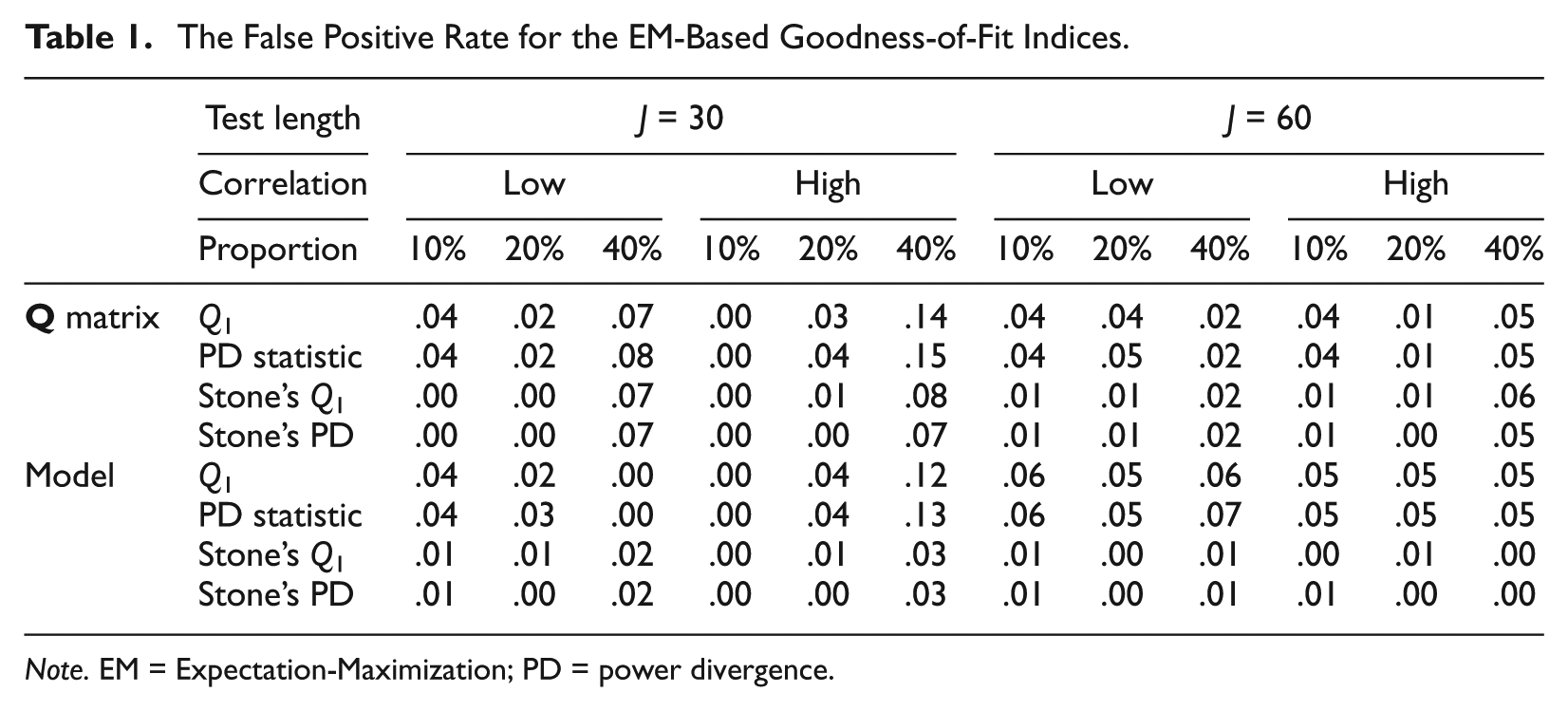
Note. EM = Expectation-Maximization; PD = power divergence.

Table 2.

The Correct Detection Rate for the EM-Based Goodness-of-Fit Indices.

	Test length	J = 30						J = 60
	Correlation	Low			High			Low			High
	Proportion	10%	20%	40%	10%	20%	40%	10%	20%	40%	10%	20%	40%
Q matrix	Q ₁	.71	.80	.63	.75	.77	.72	.96	.94	.91	.94	.94	.87
	PD statistic	.73	.83	.63	.76	.79	.74	.96	.94	.91	.95	.94	.88
	Stone’s Q₁	1.00	.99	.89	1.00	.99	.88	1.00	1.00	.98	1.00	1.00	.95
	Stone’s PD	.99	.99	.89	1.00	.99	.88	1.00	1.00	.98	1.00	1.00	.95
Model	Q ₁	.23	.29	.15	.20	.23	.31	.73	.51	.60	.71	.72	.76
	PD statistic	.23	.34	.18	.31	.25	.35	.76	.56	.62	.77	.77	.83
	Stone’s Q₁	.88	.83	.89	.97	1.00	.99	.96	.97	.97	1.00	1.00	1.00
	Stone’s PD	.87	.85	.89	.98	1.00	.99	.96	.97	.97	1.00	1.00	1.00

Note. EM = Expectation-Maximization; power divergence.

More interestingly, the empirical power, under model misspecification conditions, tended to be low for short test length and low correlation (actually extremely low without Stone’s method). The primary reason is that the correct detection of misfitting items due to a misspecified model relies more heavily on the correct recovery of $\hat{α}$ than the detection of misfitting items due to a misspecified Q matrix. For instance, suppose an item has a correct Q vector of (1, 1, 0, 0, 0), and a misspecified Q vector of (1, 0, 0, 0, 0). Then to correctly detect this misfitting item, only the second attribute needs to be correctly recovered for examinees because only examinees with and without mastering the second attribute have different correct response probabilities when the Q vector is incorrectly specified. For the same item, if the underlying model is misspecified from the DINO to the DINA model, then both the first and the second attributes need to be precisely recovered because examinees mastering either one or both the attributes will have different correct response probability from examinees mastering neither of the attributes. High correlation tends to be helpful because when the attributes were highly correlated, the entire mastery pattern, $\hat{α}$ , could be recovered more precisely by “borrowing strength” from other attributes yielding a higher empirical power.

The false positive rate and detection rate obtained from the PPMC method are presented in Tables 3 and 4. In general, the PPMC method produced comparable false positive rates as opposed to the classical approach, but with much lower detection rate. This is because the PPP values were shown to be conservative with most values around .5. The general trends of the manipulated conditions stayed the same, and they were summarized as follows: Increasing the test length and decreasing the proportion of misfitting items increased the power, using Stone’s method dramatically improved the power, there was no appreciable difference between the two discrepancy measures, and the level of correlation did not seem to have a clear effect on the performance of the PPMC method.

Table 3.

The False Positive Rate for the PPMC Method.

	Test length	J = 30						J = 60
	Correlation	Low			High			Low			High
	Proportion	10%	20%	40%	10%	20%	40%	10%	20%	40%	10%	20%	40%
Q matrix	Q ₁	.05	.07	.08	.03	.03	.04	.04	.06	.06	.03	.03	.04
	PD statistic	.06	.08	.08	.03	.03	.04	.04	.07	.06	.02	.03	.04
	Stone’s Q₁	.00	.08	.07	.00	.06	.06	.02	.12	.17	.02	.09	.09
	Stone’s PD	.00	.09	.07	.00	.06	.06	.02	.13	.18	.02	.09	.09
Model	Q ₁	.06	.04	.05	.03	.02	.02	.02	.04	.05	.03	.03	.04
	PD statistic	.06	.05	.05	.03	.03	.02	.03	.05	.05	.03	.03	.04
	Stone’s Q₁	.00	.00	.00	.00	.00	.00	.01	.06	.10	.00	.05	.06
	Stone’s PD	.00	.00	.00	.00	.00	.00	.01	.06	.11	.01	.06	.06

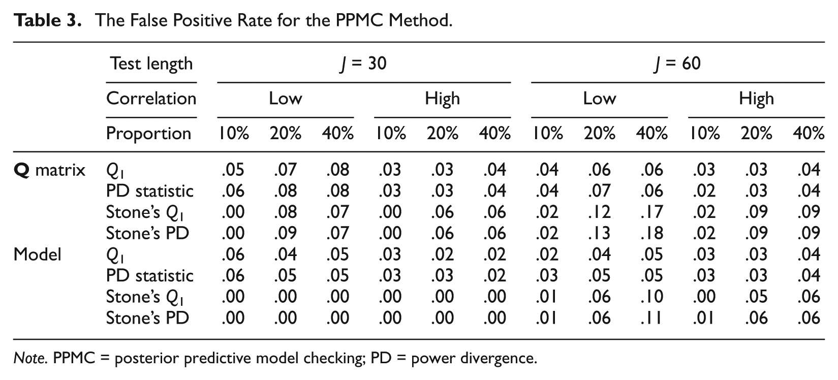
Note. PPMC = posterior predictive model checking; PD = power divergence.

Table 4.

The Correct Detection Rate for the PPMC Method.

	Test length	J = 30						J = 60
	Correlation	Low			High			Low			High
	Proportion	10%	20%	40%	10%	20%	40%	10%	20%	40%	10%	20%	40%
Q matrix	Q ₁	.07	.19	.10	.06	.07	.06	.34	.23	.10	.16	.08	.05
	PD statistic	.11	.19	.09	.06	.07	.06	.36	.25	.10	.17	.09	.05
	Stone’s Q₁	.93	.78	.15	.76	.54	.21	.95	.87	.53	.69	.64	.31
	Stone’s PD	.94	.83	.16	.76	.58	.22	.95	.89	.56	.77	.69	.32
Model	Q ₁	.38	.47	.46	.20	.21	.25	.43	.43	.32	.33	.30	.29
	PD statistic	.39	.47	.47	.18	.22	.24	.46	.46	.33	.33	.29	.29
	Stone’s Q₁	.65	.76	.76	.75	.81	.66	.92	.91	.68	.77	.72	.52
	Stone’s PD	.65	.76	.76	.75	.80	.65	.92	.92	.70	.77	.76	.53

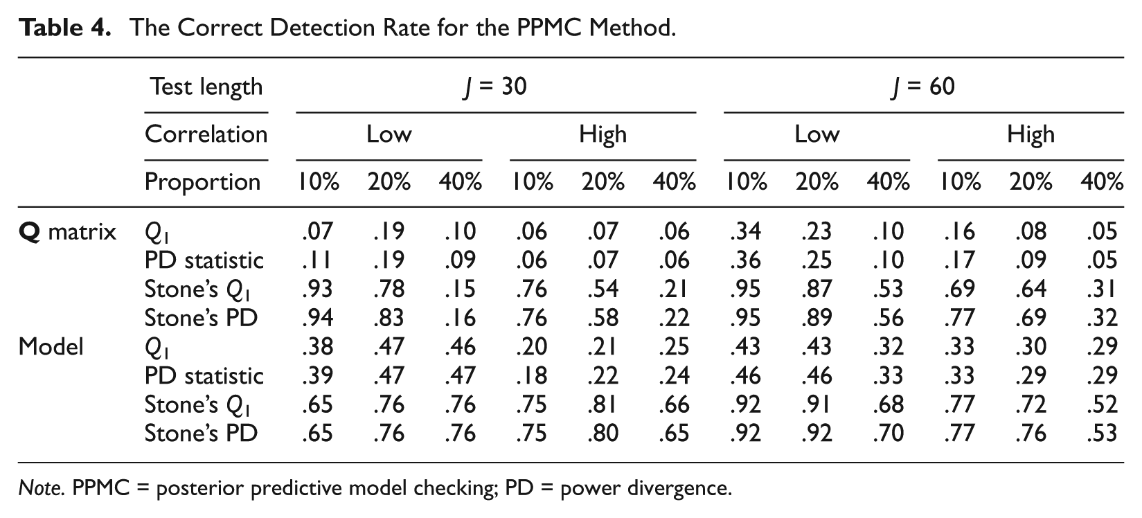
Note. PPMC = posterior predictive model checking; PD = power divergence.

From the results, the classical goodness-of-fit method should be preferred to the PPMC method. One possible reason is the PPP value does not behave like a p value in a typical hypothesis testing framework (Hjort, Dahl, & Steinbakk, 2006; Muthén & Asparouhov, 2012) because the actual Type I error rate for a correct model is not the nominal significance level. Furthermore, there is no rigorous supporting theory showing how the PPP values vary when the model/Q matrix is significantly ill-fitting at certain levels, thus PPP value is more akin to a fit index (such as RMSEA, which is compared with a cut-off value) rather than a p value.

A real data example illustrating the item-fit analysis methods using the fraction-subtraction data is provided in the online appendix, with detailed steps, results, and discussions.

Discussion

Over the past 30 years, obtaining diagnostic information from examinees’ item responses has become an increasingly important feature of educational and psychological testing. For instance, in addition to providing a summary score for accountability purpose, providing diagnostic information to promote instructional improvement becomes an important goal of the next-generation assessment. Diagnostic classification modeling, a family of restricted latent class models, has been widely recognized as one promising future direction. DCMs contain “latent variables that typically operationalize more narrowly defined constructs—so that each item requires multiple component skills” (Rupp & Templin, 2008, p. 230). Because of the finer grained dichotomy of latent spaces and the within-item dimensionalities, DCMs are known to poorly retrofit assessments originally designed for broadly based, IRT traits. To implement DCMs in real testing scenarios, model-data fit should be carefully checked and scrutinized. Very recently, Chen et al. (2013) evaluated both the relative and absolute fit of DCMs focusing on the model-level fit. They checked −2 log likelihood, Akaike information criterion (AIC), Bayesian information criterion (BIC), and residuals-based statistics, and their simulation results showed that all these indices can detect misspecification efficiently. As they acknowledged, “investigation of fit statistics at the item level is needed to fine-tune detection of model or Q-matrix misspecifications” (Chen et al., 2013), and therefore, the goal of this study is to further add to the extant literature on the item-fit checking for DCMs.

Given the fact that most DCMs are usually estimated either via the EM algorithm or the MCMC algorithm, this study evaluates two discrepancy measures coupled with both estimation algorithms. One innovation of the current approach is to apply Stone’s method in the context of DCMs so as to avoid inflated Type I and Type II errors introduced by fallible latent profile estimates. The results showed that the PPMC method was less sensitive than classical goodness-of-fit checking in detecting model/Q-matrix misspecification.

Future studies can be expanded in a number of ways. First, only two discrepancy indices were considered, whereas Kunina-Habenicht et al. (2012) explored the performance of the MAD and RMSEA and found they both exhibit high power of detecting misfitting items. Thus, it will be interesting to compare the present study’s discrepancy measures against theirs side-by-side. Second, even though the proposed item-fit analysis procedures are not restricted to any specific DCM, simulation studies were carried out only for the DINA model. Therefore, future studies can consider more flexible and complex models, such as the generalized DINA model (de la Torre, 2011), or the log-linear cognitive diagnosis model (Henson et al., 2009). Moreover, in the simulation study, Q matrix was assumed to exhibit independence structure; thus, it is interesting to evaluate the performance of the proposed methods when the attributes are correlated or display hierarchical structure (Templin & Bradshaw, 2014). Third, severity of item misfit was not differentiated when evaluating the power, whereas future study should further explore the power of the methods in identifying items with varying degree of misspecification. Items with certain types of Q-matrix misspecification (Rupp & Templin, 2008), or certain number of attributes misspecified, might be harder to detect than the others. Fourth, the authors did not consider misspecification of K (i.e., completely missing or over-specifying certain attributes), or α (i.e., incorrectly specifying certain continuous traits as binary traits) in the current simulation study and it is worth further investigation. Last but not least, while item-fit analysis is often used for sanity check purposes, statistical procedures have been proposed to estimate the optimal Q matrix directly from the observed data (de la Torre, 2008; J. Liu et al., 2012), or to correct for model misspecification at item level (de la Torre & Lee, 2013). It would be stimulating to see how these available procedures can be used jointly with the item-fit analysis discussed in this study to improve the model-data fit, or to improve the detection of misfitting items, across a wide range of settings.

Footnotes

Declaration of Conflicting Interests

The author(s) declared no potential conflicts of interest with respect to the research, authorship, and/or publication of this article.

Funding

The author(s) disclosed receipt of the following financial support for the research, authorship, and/or publication of this article: This project is partially supported by 2010 CTB/McGraw-Hill R&D research grant.

Supplemental Material

The online appendix is available at

Notes

References

Akaike

(1974). A new look at the statistical model identification. IEEE Transactions on Automatic Control, 19, 716-723.

Chen

Torre

Zhang

(2013). Relative and absolute fit evaluation in cognitive diagnosis modeling. Journal of Educational Measurement, 50, 123-140.

Collins

L. M.

Fidler

P. L.

Wugalter

S. E.

Long

J. D.

(1993). Goodness-of-fit testing for latent class models. Multivariate Behavioral Research, 28, 375-389.

Cui

Leighton

J. P.

(2009). The hierarchy consistency index: Evaluating person fit for cognitive diagnostic assessment. Journal of Educational Measurement, 46, 429-449.

de la Torre

(2008). An empirically based method of Q-matrix validation for the DINA model: Development and applications. Journal of Educational Measurement, 45, 343-362.

de la Torre

(2009). DINA model and parameter estimation: A didactic. Journal of Educational and Behavioral Statistics, 34, 115-130. doi:10.3102/1076998607309474

de la Torre

(2011). The generalized DINA model framework. Psychometrika, 76, 179-199.

de la Torre

Douglas

J. A.

(2004). Higher-order latent trait models for cognitive diagnosis. Psychometrika, 69, 333-353.

de la Torre

Douglas

J. A.

(2008). Model evaluation and multiple strategies in cognitive diagnosis: An analysis of fraction subtraction data. Psychometrika, 73, 595-624.

10.

Haertel

(1989). Using restricted latent class models to map the skill structure of achievement items. Journal of Educational Measurement, 26, 333-352.

11.

Henson

R. A.

(2008). Functions of estimating log-linear cognitive diagnostic model. Greensboro: Department of Educational Research Methodology, The University of North Carolina at Greensboro

12.

Henson

R. A.

Templin

J. L.

Willse

J. T.

(2009). Defining a family of cognitive diagnosis models using log-linear models with latent variables. Psychometrika, 74, 191-210.

13.

Hjort

N. L.

Dahl

F. A.

Steinbakk

G. H.

(2006). Post-processing posterior predictive p values. Journal of the American Statistical Association, 101, 1157-1174.

14.

Hong

Wang

Lim

Douglas

(2015). Efficient models for cognitive diagnosis with continuous and mixed-type latent variables. Applied Psychological Measurement, 39, 31-43.

15.

Junker

B. W.

Sijtsma

(2001). Cognitive assessment models with few assumptions, and connections with nonparametric item response theory. Applied Psychological Measurement, 25, 258-272.

16.

Kunina-Habenicht

Rupp

A. A.

Wilhelm

(2012). The impact of model misspecification on parameter estimation and item-fit assessment in log-linear diagnostic classification models. Journal of Educational Measurement, 49, 59-81.

17.

Levy

Mislevy

R. J.

Sinharay

(2009). Posterior predictive model checking for multidimensionality in item response theory. Applied Psychological Measurement, 33, 519-537.

18.

Liu

You

Wang

Ding

Chang

H.-H.

(2014). Large-scale implementation of computerized adaptive testing with cognitive diagnosis in China. In Cheng

Chang

H.-H.

(Eds.), Advanced methodologies to support both summative and formative assessments (pp. 245-261). Charlotte, NC: Information Age.

19.

Liu

Ying

(2012). Data-driven learning of Q-matrix. Applied Psychological Measurement, 36, 548-564.

20.

Liu

Douglas

Henson

(2009). Testing person fit in cognitive diagnosis. Applied Psychological Measurement, 33, 579-598.

21.

Maris

(1999). Estimating multiple classification latent class models. Psychometrika, 64, 187-212.

22.

McKinley

R. L.

Mills

C. N.

(1985). A comparison of several goodness-of-fit statistics. Applied Psychological Measurement, 9, 49-57.

23.

Meng

X.-L.

(1994). Posterior predictive p-values. The Annals of Statistics, 3, 1142-1160.

24.

Muthén

Asparouhov

(2012). Bayesian structural equation modeling: A more flexible representation of substantive theory. Psychological Methods, 17, 313-335.

25.

Oliveri

M. E.

von Davier

(2011). Investigation of model fit and score scale comparability in international assessment. Psychological Test and Assessment Modeling, 53, 315-333.

26.

Orlando

Thissen

(2000). Likelihood-based item-fit indices for dichotomous item response theory models. Applied Psychological Measurement, 24, 48-62.

27.

Read

T. R.

Cressie

N. A.

(1988). Goodness-of-fit statistics for discrete multivariate data. New York, NY: Springer.

28.

Reckase

M. D.

(2009). Multidimensional item response theory. New York, NY: Springer.

29.

Robins

J. M.

van der Vaart

Ventura

(2000). Asymptotic distribution of P values in composite null models. Journal of the American Statistical Association, 95, 1143-1156.

30.

Roussos

L. A.

DiBello

L. V.

Stout

Hartz

S. M.

Henson

R. A.

Templin

(2007). The fusion model skills diagnosis system. In Leighton

J. P.

Gierl

M. J.

(Eds.), Cognitive diagnostic assessment for education: Theory and applications (275-318). Cambridge, UK: Cambridge University Press.

31.

Roussos

L. A.

Templin

J. L.

Henson

R. A.

(2007). Skills diagnosis using IRT-based latent class models. Journal of Educational Measurement, 44, 293-311.

32.

Rupp

Templin

(2008). The effects of Q-matrix misspecification on parameter estimates and classification accuracy in the DINA model. Educational and Psychological Measurement, 1, 78-96.

33.

Rupp

A. A.

Templin

Henson

R. A.

(2010). Diagnostic measurement: Theory, methods, and applications. New York, NY: Guilford Press.

34.

Schwarz

(1978). Estimating the dimension of a model. The Annals of Statistics, 6, 461-464.

35.

Sinharay

(2006). Model diagnosis for Bayesian Networks. Journal of Educational and Behavioral Statistics, 31, 1-33.

36.

Sinharay

Almond

R. G.

(2007). Assessing fit of cognitive diagnostic models: A case study. Educational and Psychological Measurement, 67, 239-257.

37.

Sinharay

Johnson

M. S.

Stern

H. S.

(2006). Posterior predictive assessment of item response theory models. Applied Psychological Measurement, 30, 298-321.

38.

Spiegelhalter

D. J.

Best

N. G.

Carlin

B. P.

Van Der Linde

(2002). Bayesian measures of model complexity and fit. Journal of the Royal Statistical Society: Series B (Statistical Methodology), 64, 583-639.

39.

Stone

C. A.

(2000). Monte Carlo based null distribution for an alternative goodness-of-fit test statistic in IRT models. Journal of Educational Measurement, 37, 58-75.

40.

Templin

Bradshaw

(2014). Hierarchical diagnostic classification models: A family of models for estimating and testing attribute hierarchies. Psychometrika, 79, 317-339.

41.

Templin

J. L.

Henson

R. A.

Templin

S. E.

Roussos

(2008). Robustness of hierarchical modeling of skill association in cognitive diagnosis models. Applied Psychological Measurement, 32, 559-574. doi:10.1177/0146621607300286

42.

Toribio

Albert

(2011). Discrepancy measures for item fit analysis in item response theory. Journal of Statistical Computation and Simulation, 81, 1345-1360.

43.

Torre

Lee

Y. S.

(2013). Evaluating the Wald test for item-level comparison of saturated and reduced models in cognitive diagnosis. Journal of Educational Measurement, 50, 355-373.

44.

von Davier

(2008). A general diagnostic model applied to language testing data. British Journal of Mathematical and Statistical Psychology, 61, 287-307.

45.

Wang

(2013). Mutual information item selection method in cognitive diagnostic computerized adaptive testing with short test length. Educational and Psychological Measurement, 73, 1017-1035.

46.

Wang

Chang

H. H.

Huebner

(2011). Restrictive stochastic item selection methods in cognitive diagnostic computerized adaptive testing. Journal of Educational Measurement, 48, 255-273.

47.

Wang

Nydick

(2015). Comparing two algorithms for calibrating the restricted non-compensatory multidimensional IRT model. Applied Psychological Measurement, 39, 119-134.

48.

Yen

W. M.

(1981). Using simulation results to choose a latent trait model. Applied Psychological Measurement, 5, 245-262.

Supplementary Material

Please find the following supplemental material available below.

For Open Access articles published under a Creative Commons License, all supplemental material carries the same license as the article it is associated with.

For non-Open Access articles published, all supplemental material carries a non-exclusive license, and permission requests for re-use of supplemental material or any part of supplemental material shall be sent directly to the copyright owner as specified in the copyright notice associated with the article.

0.00 MB

0.52 MB