Maximum Likelihood Score Estimation Method With Fences for Short-Length Tests and Computerized Adaptive Tests

Abstract

A critical shortcoming of the maximum likelihood estimation (MLE) method for test score estimation is that it does not work with certain response patterns, including ones consisting only of all 0s or all 1s. This can be problematic in the early stages of computerized adaptive testing (CAT) administration and for tests short in length. To overcome this challenge, test practitioners often set lower and upper bounds of theta estimation and truncate the score estimation to be one of those bounds when the log likelihood function fails to yield a peak due to responses consisting only of 0s or 1s. Even so, this MLE with truncation (MLET) method still cannot handle response patterns in which all harder items are correct and all easy items are incorrect. Bayesian-based estimation methods such as the modal a posteriori (MAP) method or the expected a posteriori (EAP) method can be viable alternatives to MLE. The MAP or EAP methods, however, are known to result in estimates biased toward the center of a prior distribution, resulting in a shrunken score scale. This study introduces an alternative approach to MLE, called MLE with fences (MLEF). In MLEF, several imaginary “fence” items with fixed responses are introduced to form a workable log likelihood function even with abnormal response patterns. The findings of this study suggest that, unlike MLET, the MLEF can handle any response patterns and, unlike both MAP and EAP, results in score estimates that do not cause shrinkage of the theta scale.

Keywords

estimation scoring computerized adaptive testing

Introduction

For score estimation based on the item response theory (IRT), the maximum likelihood estimation (MLE) method is one of the most frequently used methods because of its ability to provide unbiased estimates. A critical shortcoming of MLE, however, is that it cannot handle certain response strings, including ones that consist only of all 0s or all 1s. This is especially problematic when the test length is short (e.g., 10 or fewer items). It can also be problematic, for example, in the early stages of administering a computerized adaptive testing (CAT), when just a few responses have been recorded, resulting in an increased chance of extreme responses patterns—a situation that MLE cannot handle.

To date, two methods for overcoming this challenge have been put into practice, but with uneven results. The first solution establishes lower and upper bounds of theta estimation, and then assigns either the lower bound value as the estimated score when the response string consists only of 0s or the upper bound value as the score estimate if all responses are 1s. This solution, however, causes theoretical and computational discontinuation from the rest of the normal MLE estimation process. More importantly, even if a response string consists of both 0s and 1s, there are certain aberrant response patterns that the MLE method cannot handle.

A second means of handling responses with all 0s or all 1s is to use Bayesian-based estimation methods (Owen, 1975) such as the modal a posteriori (MAP; Samejima, 1969) method or the expected a posteriori (EAP; Bock & Aitkin, 1981) method. By imposing a prior distribution on the log likelihood function, MAP/EAP methods always have a peak from which to find a score estimate. The problem with this approach, however, is that the MAP or EAP methods are known to result in estimates biased toward the center of a prior distribution, resulting in a shrunken score scale (Weiss & McBride, 1984). Demands from the field for a score estimation method that can resolve these aforementioned issues are on the rise.

MLE

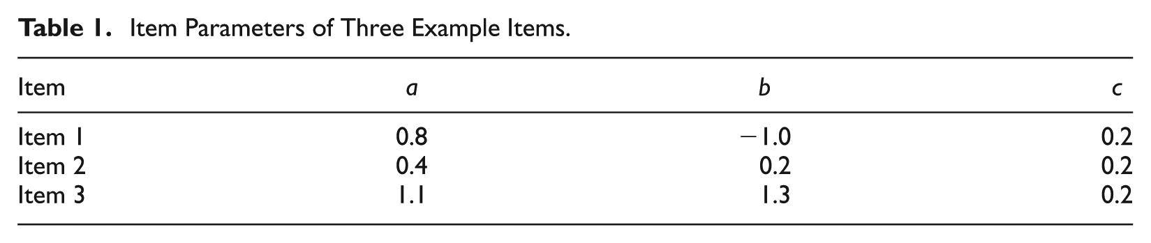
Given the administered items and examinee’s responses, the log likelihood function for a conventional MLE method is computed, for example, for unidimensional, dichotomously scored response data as follows:

L = \ln (μ | θ) = \sum_{j = 1}^{n} [μ_{j} \ln P_{j} + (1 - μ_{j}) \ln (1 - P_{j})],

where µ is a response string of j items, which is ( $μ_{1}, μ_{2}, \dots, μ_{j}$ ), and $P_{j}$ is the item response function given θ. An example of the log likelihood function with three items is illustrated in Figure 1. The item parameters—based on the three-parameter logistic model (3PLM; Birnbaum, 1968)—for this example are reported in Table 1. In Figure 1, when the response string was (1, 1, 0), the θ value that corresponds to the location of the peak of the log likelihood function (i.e., maximized log likelihood value)— $\ln (μ = (1, 0, 0) | θ)$ —was about −0.4. Conceptually, that is how MLE works. In practice, the MLE is usually found via the Newton–Raphson method (or Fisher’s method of scoring, which essentially is the same as the Newton–Raphson method in this situation; Baker & Kim, 2004; Kendall & Stuart, 1967). In the Newton–Raphson method, the score estimate, $\hat{θ}$ , is updated as the process iterates t-th time:

{[\hat{θ}]}_{t + 1} = {[\hat{θ}]}_{t} - {[\frac{\partial^{2} L}{\partial θ^{2}}]}_{t}^{- 1} \times {[\frac{\partial L}{\partial θ}]}_{t} .

Figure 1.

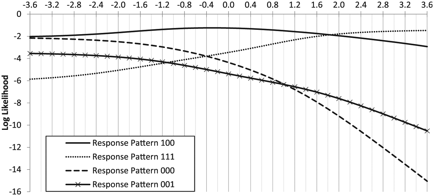
Log likelihood functions of three-item response patterns.

Table 1.

Item Parameters of Three Example Items.

Item	a	b	c
Item 1	0.8	−1.0	0.2
Item 2	0.4	0.2	0.2
Item 3	1.1	1.3	0.2

As shown in Figure 1, when the response string is (1, 1, 1), the log likelihood function value continuously increases as θ approaches infinity. Also, when the response string is (0, 0, 0), the log likelihood function value keeps increasing as θ approaches negative infinity. In cases where the response string (µ) consists of only 1s or only 0s, there is no definite peak; as a result, the MLE method fails to find a definite solution for θ. To address this issue with the MLE method, a $\hat{θ}$ distribution is almost always truncated by placing the lower and upper bounds (e.g., a lower bound at −3.0 and a upper bound at 3.0). With this modification, the lower bound value is “assigned” as the $\hat{θ}$ for the examinees whose response string consists of only 0s (i.e., answering all items incorrectly). Those examinees whose response string consists of only 1s (i.e., answering all items correctly) get the upper bound value as their $\hat{θ}$ . This definition-based solution for MLE, however, cannot be applied to cases in which a response string includes both 0s and 1s. Some response strings may include both 0s and 1s but still not have a definite peak on the log likelihood function. For example, examining response pattern (0, 0, 1) in which the examinee answered two easier items (Items 1 and 2) incorrectly and the harder item (Item 3) correctly, we can see that the log likelihood function keeps increasing as θ approaches negative infinity (Figure 1). As a result, the MLE estimate does not exist.

MLE With Fences (MLEF)

An alternative method, henceforth referred to as the maximum likelihood estimation with fences (MLEF), basically functions the same as MLE with the following exception. Instead of placing the fixed upper and lower bounds to truncate the $\hat{θ}$ scale, the MLEF puts in place two imaginary items with fixed responses to establish “fences” around a meaningful range of the log likelihood function for score estimation. The use of imaginary items and responses when the MLE estimator is unavailable is not new to the field; some practitioners proposed a similar approach for selecting the next item after the first item administration in CAT (Herrando, 1989; Olea & Ponsoda, 2003). In MLEF, the first imaginary item serves as the lower fence and its b parameter is set at θ, where the lower bound of the θ distribution is expected (e.g., b = −3.5). For the b-parameter value, the lower fence should be lower than any items in the test form. Likewise, the second imaginary item serves as the upper fence, and its b parameter is set at θ, where the upper bound of the θ distribution is expected (e.g., b = 3.5). The b-parameter upper fence value should be larger than any items in the test form. These two “fence” items should be set to have a very high a-parameter value (e.g., a = 3.0). Additional discussion about the choice of a-parameter value of the fence items appears in the latter part of this article. For the lower fence item, the response is always fixed at “1” and the upper fence item response is fixed at “0.” With the MLEF, the log likelihood function (Equation 1), thus, can be rewritten as follows:

L^{*} = \ln P_{LF} + \ln (1 - P_{UF}) + \sum_{j = 1}^{n} [μ_{j} \ln P_{j} + (1 - μ_{j}) \ln (1 - P_{j})],

where $P_{LF}$ and $P_{UF}$ are the item response functions of the lower and upper fences, respectively. With this modification, the log likelihood functions from the earlier example in Figure 1 are changed, as shown in Figure 2. For the response string (1, 0, 0), the log likelihood function from Equation 3 (Figure 2) is nearly identical to the one based on Equation 1 (Figure 1), and as a result, $\hat{θ}$ is the same as well (≈−0.4). The cases with the response patterns (0, 0, 0), (1, 1, 1), and (0, 0, 1), in which the MLE estimate does not exist with Equation 1, now have identifiable peaks with Equation 3; as a result, MLE estimates exist for all of the response patterns.

Figure 2.

Log likelihood functions of three-item response patterns with fences.

The MLEF method has several interesting characteristics in comparison with some Bayesian-based estimation methods, such as the MAP. In the MAP method, the prior density information is imposed in the log likelihood function computation, whereas, in the MLEF method, the prior information regarding range of θ scale is reflected in $P_{LF}$ and $P_{UF}$ . Unlike the prior density information in MAP that influences the log likelihood function across the entire θ scale, the influence of the fences in MLEF is limited to the areas where the fences are located. Further discussion about the theoretical and practical differences between MAP and MLEF follows in the latter part of this article.

To investigate and evaluate the performance and behavior of MLEF in comparison with other established estimation methods, a series of simulation studies were conducted.

Study 1: Short, Fixed-Length Test

Data and Method

Study 1 examined the behavior and performance of MLEF compared with MLE (with and without truncation at −3.5 and 3.5), MAP, and EAP (with a standard normal distribution as a prior), when the test length was very short (between one and 10 items). The same 10 items that were administered to 7,000 simulees were drawn from a uniform distribution (−3.5, 3.5), and the 10 items were based on the 3PLM (Birnbaum, 1968) with b-parameter values ranging from −2.7 to 2.7 with an interval of 0.6 (see Table 2 for item parameters). The a- and c-parameter values were set at 1.0 and 0.2 for all items, respectively. The θ was estimated after each item administration to observe the interaction between the studied estimation methods and test length. The sequence of the 10 items was randomized across simulated test takers to cancel out the item effect from the test-length effect.

Table 2.

Item Parameters of the Short, Fixed-Length Test in Study 1.

Item	a	b	c
Item 1	1.0	−2.7	0.2
Item 2	1.0	−2.1	0.2
Item 3	1.0	−1.5	0.2
Item 4	1.0	−0.9	0.2
Item 5	1.0	−0.3	0.2
Item 6	1.0	0.3	0.2
Item 7	1.0	0.9	0.2
Item 8	1.0	1.5	0.2
Item 9	1.0	2.1	0.2
Item 10	1.0	2.7	0.2

For the condition with MLE, the Newton–Raphson method was used to find MLE. In the Newton–Raphson algorithm, the maximum absolute magnitude of update (the second term on the right-hand side of Equation 2) for each iteration was limited to 1, and the estimation procedure was iterated up to 20 times with the initial value set at 0.0. If the magnitude of update became smaller than 0.001, the estimation was considered converged and the Newton–Raphson cycle was stopped. In another condition—MLE with truncation (MLET)—everything was the same as the MLE condition except that $\hat{θ}$ was forced to be between −3.5 and 3.5 during and after the Newton–Raphson procedure.

For the condition based on the Bayesian methods MAP and EAP, the prior density was set to follow N(0, 1). For the MAP condition, everything else was the same as the MLE condition (maximum of 20 iterations of the Newton–Raphson procedure with a maximum update magnitude of 1 for each iteration). For the EAP condition, 40 quadrature points between −4.0 and 4.0 were used.

The condition with MLEF used two (imaginary) fence items. The b parameter for the lower fence was −3.5; for the upper fence, it was 3.5. The a-parameter value was 3.0 for both fences. All other configurations remained the same as the MLE condition.

Once the θ estimation was performed under each condition, the estimation bias and the mean absolute error (MAE) statistics were computed and evaluated for each θ area. The simulation was implemented using the computer software, SimulCAT (Han, 2012), which is publicly available.

Results

The MLE condition in this study was not truly unrestricted on the scale of $\hat{θ}$ . Because the maximum magnitude of update for each iteration of the Newton–Raphson procedure was set to 1 and because the procedure was finished after 20 iterations, the actual scale of $\hat{θ}$ under the MLE condition was between −20.0 and 20.0. This factor should be considered when interpreting the results from the MLE condition. As shown in Figure 3, θ in MLE tends to be outrageously underestimated when θ < 0 and also tends to be hugely overestimated when θ > 0. This mainly results when the log likelihood function does not have an identifiable peak, meaning the $\hat{θ}$ is either −20 or 20. When the $\hat{θ}$ is between −2.5 and 3.5 under the MLET condition, there is practically no estimation bias across all θ areas when the number of administered items exceeds five. When −3.5 ≤θ < −2.5 (Area −3 in Figure 3), MLET shows small estimation bias even when all 10 items are administered. It was a much anticipated phenomenon of 3PLM, where the lower asymptote of response function results in asymmetrical log likelihood functions (MLE-based approaches focus only on the peak of log likelihood function).

Figure 3.

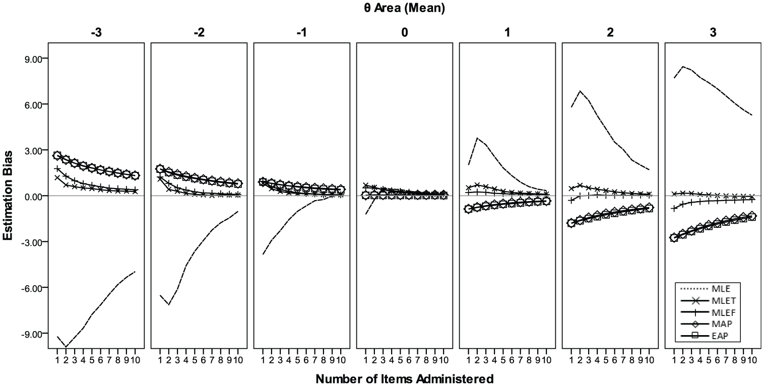
Conditional bias in score estimation for a test with 10 items with random sequence.

The MAP and EAP conditions resulted in almost identical estimation bias patterns when compared with each other. Because of the role of prior density information, the estimates were pulled toward the center of the prior (“0” in this study); as a result, θ was underestimated when θ > 0 and overestimated when θ < 0. This observation concurs with the property of Bayesian-based estimation methods, known as the shrinkage of scale (Baker & Kim, 2004; McBride, 1977; Novick & Jackson, 1974; Weiss & McBride, 1984). The estimation bias with MAP and EAP persisted even after all 10 items were administered when θ was far from the center of prior.

The estimation bias with the MLEF condition shows a pattern similar to the MLET condition (Figure 3). MLEF seemed to show slightly larger bias than MLET when θ was extreme (e.g., Areas −3 and 3) and when the test length was extremely short (<5 items). Most of the bias diminished across θ areas as the test length reach 10 items, however.

As shown in Figure 4, the MAEs with the MAP and EAP conditions moderately increased as $| θ |$ was further away from the center of prior. When 2.5 ≤ $| θ |$ < 3.5 (Areas −3 and 3 in Figure 4), the MAE with MAP and EAP was still much larger than 1.0 after all 10 items were administered mainly because of the large estimation bias shown in Figure 3. In those extreme θ areas, MLET and MLEF showed the smallest MAE among the studied conditions. When θ was near “0,” MAP and EAP resulted in the smallest MAE because it was where the center of the prior located. MLET and MLEF tend to show larger MAE in the central θ area when the number of administered items is very small (e.g., <5). In those cases, there was a greater chance that those methods would result in estimates that were closer to where the truncation happened (with MLET) or to where the fence items located (with MLEF). Overall, all studied estimation methods showed comparable MAE once all 10 items were administered, except for MAP and EAP when 2.5 ≤ $| θ |$ .

Figure 4.

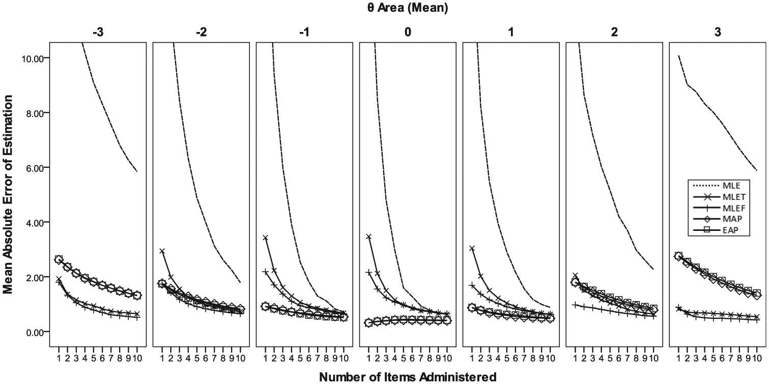
Conditional mean absolute errors of score estimation for a test with 10 items with random sequence.

Compared with MLET, MLEF tends to show slightly smaller MAE across all θ (Figure 4). Also, in terms of computation efficiency, MLEF solutions tend to get converged much faster than MLET, notably because MLEF always had an identifiable peak, especially when the test length was extremely short, for example, <5 (Figure 5).

Figure 5.

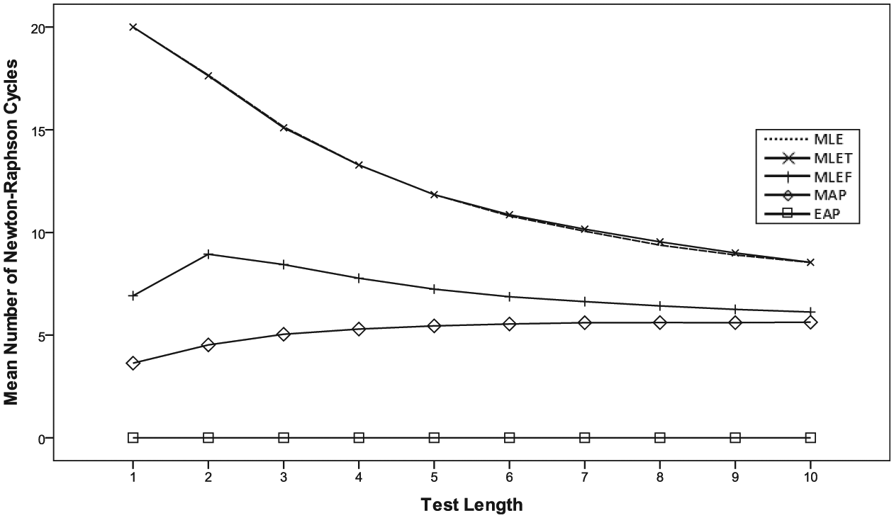
Average number of Newton–Raphson cycles before convergence for the MLEF and MLET conditions.

Overall, the observations from Study 1 suggest that the MLEF method retains the favorable properties of MLE, such as unbiased estimation, while being robust against some response patterns that pose a problem for typical MLE, and is capable of producing stable estimates within a very few Newton–Raphson cycles.

Study 2: CAT Simulation

Study 1 investigated test situations involving short test lengths. A more common test situation where practitioners encounter problems of MLE involves CAT. In CAT, after each item administration, an interim θ estimate needs to be computed to select the next item. Study 2 examined this situation.

Data and Method

Study 2 used the same simulee data examined in Study 1. To ensure that the results from the CAT simulation were as generalizable as possible and, more importantly, to eliminate all extraneous factors from the study, the CAT design was intentionally simplified. Item selection was based on the maximized Fisher information (MFI) criterion (Weiss, 1982). Content balancing and item exposure control were not considered. The items were based on the two-parameter logistic model (2PLM). To ensure an item pool sufficient to support ideal item selection, the item pool consisted of 800 items with b-parameter values ranging from −4.00 to 3.99 with an increment of 0.01. The test length was fixed and each administration used 30 items. As with Study 1, MLE, MLET, MAP, and EAP methods as well as MLEF were examined. All other study conditions remained the same as Study 1.

Results

With CAT, the estimation bias was close to none after about 10 to 15 item administrations under the MLE, MLET, and MLEF conditions (Figure 6). Under the MAP and EAP conditions, the magnitude of bias tended to be smaller with CAT than that observed with the non-CAT conditions from Study 1. It still persisted, however, except when θ was at the center of prior (=0). 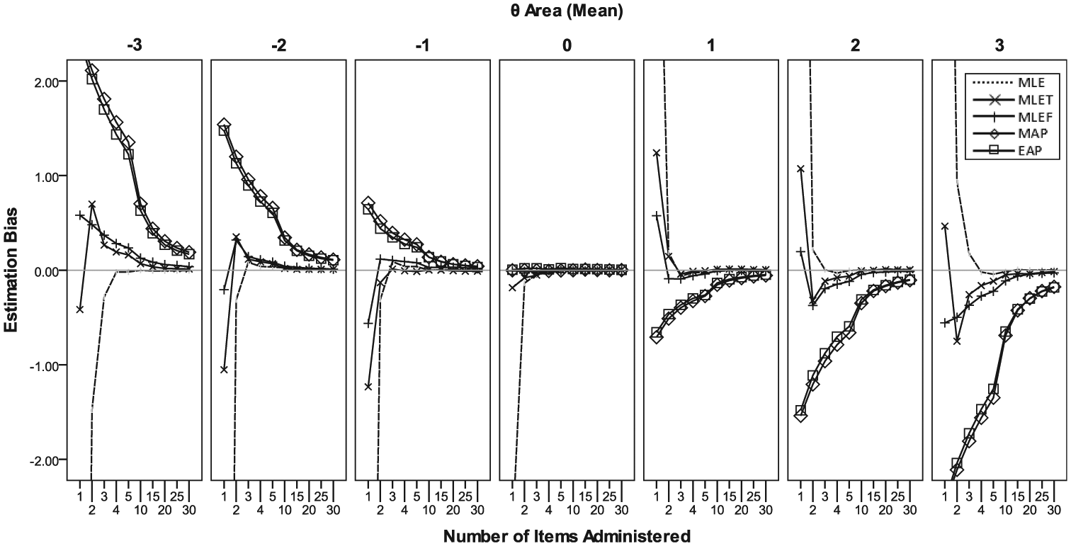In terms of the MAE, all studied estimation methods showed a similar level after close to 10 items were administered, except when 2.5 ≤ $| θ |$ (Figure 7). In the areas of 2.5 ≤ $| θ |$ , the MAP and EAP conditions resulted in MAE moderately larger than other studied methods even after 30 item administrations.

Figure 6.

Conditional bias in score estimation from Study 2 (CAT).

Figure 7.

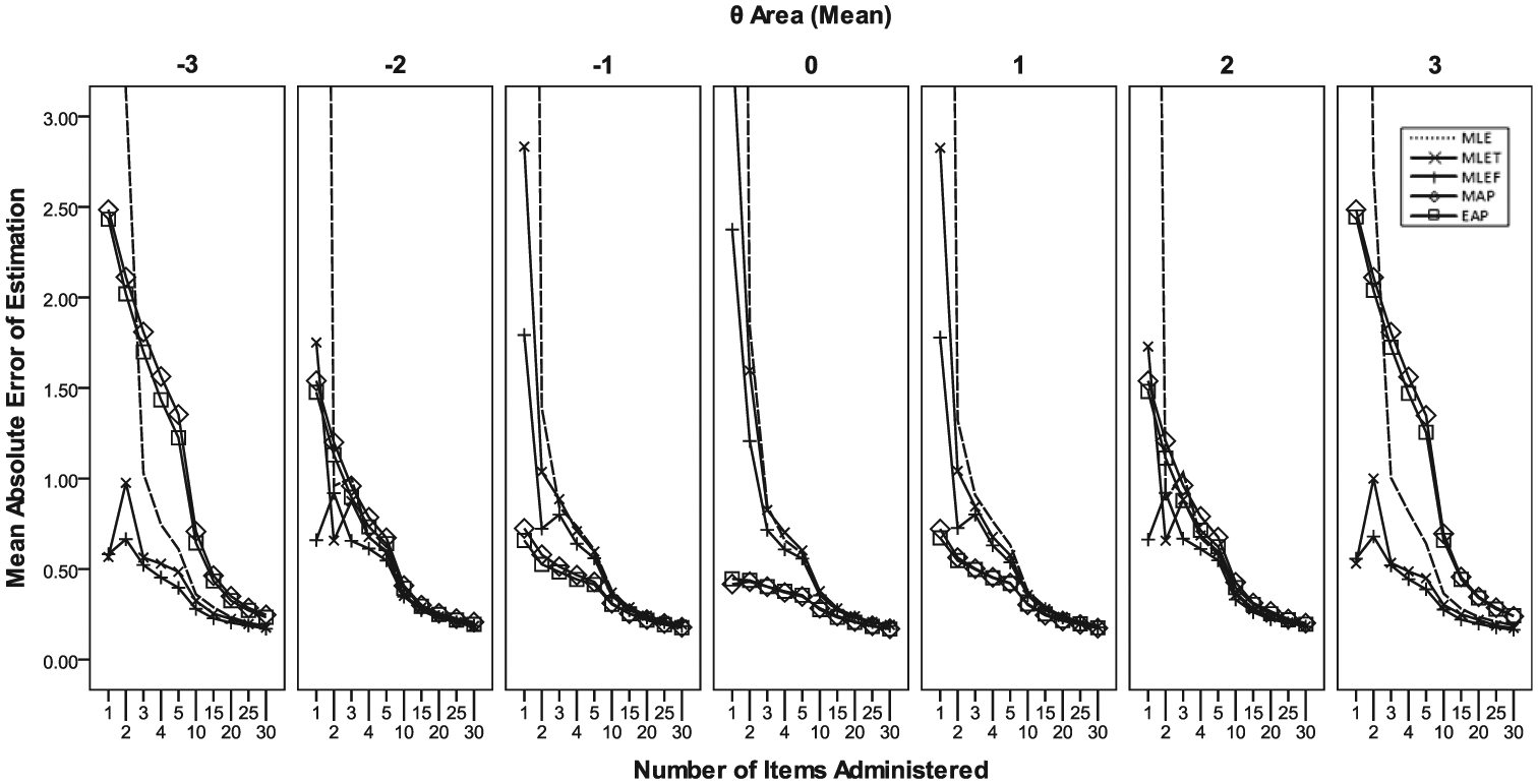
Conditional mean absolute errors of score estimation from Study 2 (CAT).

Figure 8 displays conditional MAE of final θ estimates (after 30 item administrations). Concurring with the results from previous studies (Wang & Vispoel, 1998; Weiss, 1982; Weiss & McBride, 1984), it shows that when the MAP and EAP methods were used, MAE was minimized around the center of the prior and increased as it moved away from the center. The MLE and MLET resulted in MAE that was slightly larger than the minimum MAE observed with the MAP and EAP methods but consistent across the θ scale. The MLEF condition showed an MAE pattern similar to those seen under the MLE and MLET conditions.

Figure 8.

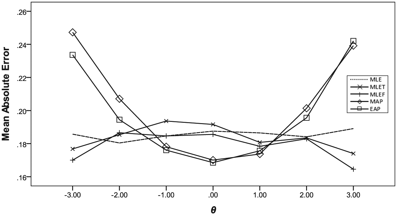
Conditional mean absolute errors of final score estimation from Study 2 (CAT).

Discussion

The results of Studies 1 and 2 reconfirmed the well-known properties of the existing estimation methods (MLE, MLET, MAP, and EAP) examined in previous studies (Wang & Vispoel, 1998; Weiss, 1982; Weiss & McBride, 1984) and revealed the behavior and performance of the MLEF method. Overall, the MLEF method exhibited the same characteristic of MLET—next to no estimation bias regardless of the test length and consistent estimation error across the θ scale. It should be noted, however, that MLEF is conceptually and computationally different from MLET, as discussed further.

Although the MLE condition (without truncation but with a restriction on the maximum magnitude of update from each Newton–Raphson cycle) was included in Studies 1 and 2, pure MLE without any restriction is rarely (if ever) used in operational testing programs due to its inability to deal with certain response patterns. MLET most often has been considered a practical alternative in real-world applications. Theoretically, MLET is a special case of MAP in which the prior probability distribution follows a uniform distribution (aka, a noninformative prior). With or without the use of the noninformative prior, however, if a log likelihood function does not have an identifiable peak, MLET will not result in a converged solution. It will still require definitional solutions, possibly with external restrictions such as the maximum number of Newton–Raphson cycles and the maximum limit in update amount of each Newton–Raphson iteration, all of which contribute to degraded efficiency of the estimation process. Also, because MLET’s definitional solutions (i.e., upper and lower bounds) treat all $\hat{θ}$ s that are outside of the bounds indifferently, many examinees with different response patterns could end up with exactly the same $\hat{θ}$ (either the upper or lower bound value).

However, with the lower and upper fences of MLEF, the log likelihood function itself (Equation 3) is transformed to always have an identifiable peak (especially when the test length is extremely short). Unlike MLET, where the upper and lower bounds are defined as absolute limits of the θ scale, the fences of MLEF technically do not place absolute limits on the scale. Instead, they help the log likelihood function form an identifiable peak between the lower and upper fences by causing substantial decrease in the log likelihood function outside of fences. Because of this, even for those examinees whose θ is close to either the lower or upper fence location, MLEF rarely results in exactly the same estimate unless the response pattern is exactly the same. With MLEF, extreme $\hat{θ}$ values keep asymptomatically increasing toward the upper fence or decreasing toward the lower fence (unlike MLET where the scale is literally truncated at the specified bounds).

Like MLET, which can be viewed as a special case of MAP (with a noninformative prior), MLEF may be viewed as another special case of MAP, as well. In addition to using directly observed response data for computing the log likelihood function, MAP incorporates a prior probability distribution. The choice of a prior of MAP has a great impact on $\hat{θ}$ throughout the scale, and as θ is further away from the center of prior; the impact of prior negatively contributes to the accuracy of estimation (unless a noninformative prior is selected; Wang, Hanson, & Lau, 1999). Although the negative influence of prior decreases proportionately as the test length increases, the estimation bias inherent in the role of prior moderately persists even after a reasonably large number of items (e.g., 30) are administered (Figures 6 and 8). MLEF, on the contrary, includes the log likelihood function values of the lower and upper fences ( $P_{LF}$ and $P_{UF}$ in Equation 3) when computing the log likelihood function as well as the directly observed response data. Based on the example shown in Figure 2, the log likelihood function of $P_{LF}$ and $P_{UF}$ shown in Figure 9 is, in a Bayesian sense, a prior information. Unlike typical choices of prior for MAP—for example, N(0, 1)—however, the influence of fences of MLEF is isolated only around the fence locations (with a large enough value for a parameter for the fence items; for example, >3). As a result, the negative impact of the fences on θ estimation across the scale is minimal. In addition, after a small number of items are administered (e.g., 5-10), most systematic errors are nearly all diminished (see Figures 3 and 6).

Figure 9.

Log likelihood function of fence items (from the example of Figure 2).

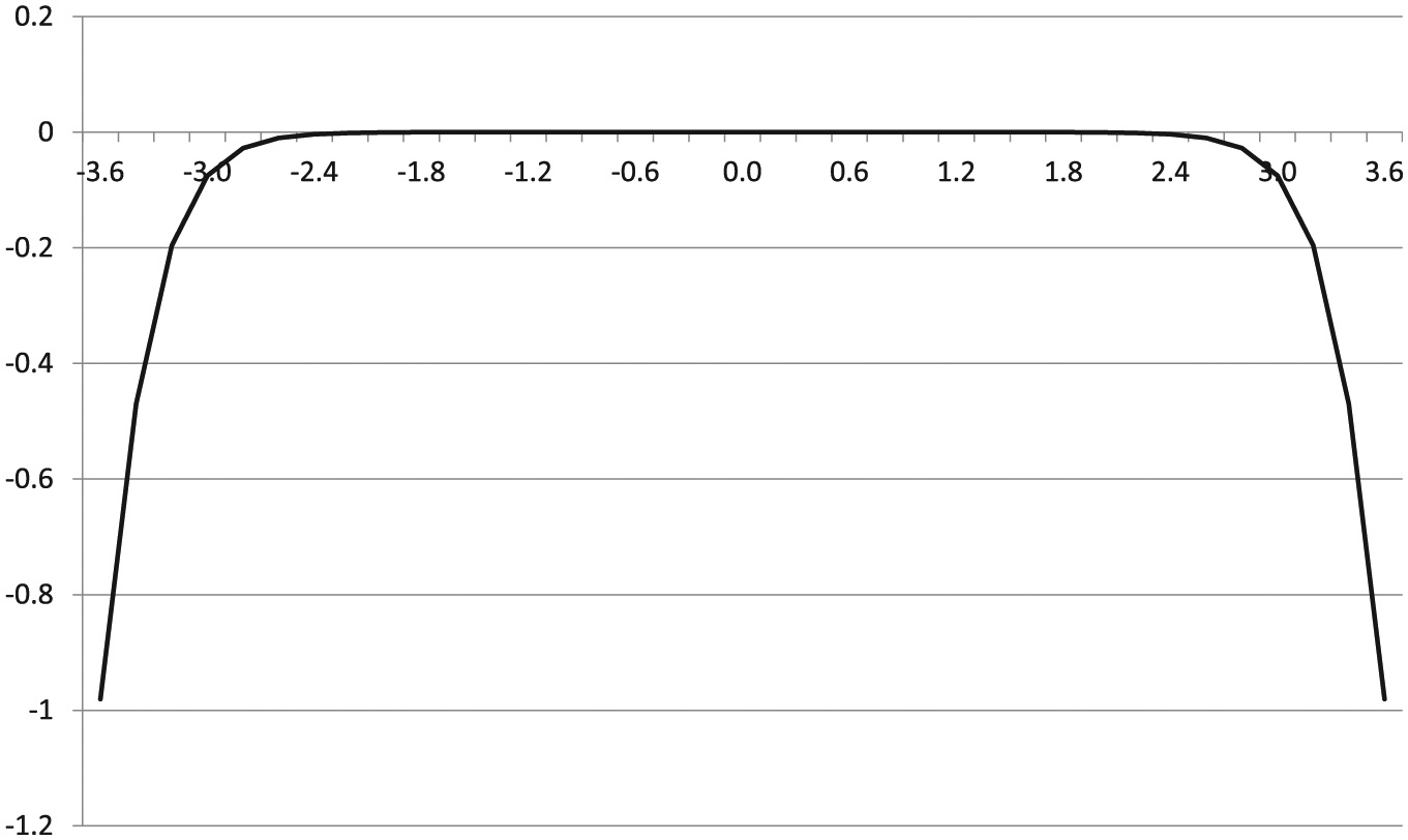
Choosing a prior for MAP is often viewed as an ambiguous process. So too is the process for setting the fences for MLEF, because it ultimately involves human judgment. In theory, a prior for MAP (or any Bayesian-based method) can be a probability distribution of any shape. In practice, however, the prior of choice most often has a symmetric bell shape like a normal distribution. Ideally, the prior distribution should reflect the population, but in real-world practice, it is often unknown or does not follow a typical normal distribution. So, it is hard to choose a prior that exactly reflects the real world. The MLEF fences, however, contain limited information only in the areas where they locate. Also, MLEF requires no assumptions on the shape of θ distribution, so it is not hard to arrive at reasonable locations for the lower and upper fences. For example, setting the lower and upper fences at −3.5 and 3.5, respectively (as in Studies 1 and 2), would be good enough for most operational cases (assuming a standard normal distribution), and the scale with fences at −3.5 and 3.5 would cover 99.95% of the population. As for the choice of a-parameter value for the fence items, this study suggests it needs to be high (e.g., a = 3.0). If the a-parameter value for the fence items is too low, for example, 0.5, the shape of log likelihood function of the two fence items (Figure 9) becomes something close to a bell shape that peaks near the center between lower and upper fences (LF and UF). If that happens, the effect of fences will not be limited within the fence locations, and as a result, MLEF will behave more like a typical MAP with a normal prior, and the distinct advantages of MLEF over MAP will be diminished. Based on the results of Studies 1 and 2, MLEF seemed reasonably effective when a = 3.0 for the fence items. A more comprehensive study to evaluate the performance and behavior of MLEF with different a-parameter values for fence items, however, is in order.

The EAP method was not extensively discussed in this article because its estimation process is quite different from the other studied methods (MLE, MLET, MLEF, and MAP). The EAP method does not use the iterative Newton–Raphson process but instead computes the conditional posterior distribution for each quadrature point to find $\hat{θ}$ at the “expected a posteriori” (i.e., mean of the posterior distribution). Despite the conceptual and computational differences between EAP and MAP, unless the mode and mean of a posterior distribution differ a lot, EAP and MAP usually result in similar estimation results (as observed in Studies 1 and 2). Thus, the consequential difference between MLEF and EAP (in terms of estimation bias and errors) parallels the difference between MLEF and MAP.

Bayesian methods such as MAP and EAP may be a more appealing choice over MLEF under the following conditions: (a) the center of prior is where it matters the most (e.g., a cut score also locates where the center of prior locates), (b) the selected prior distribution reflects the real population reasonably well, and (c) large estimation biases for examinees who are distant from the center of prior do not matter. Such a test situation is rare, however, especially under CAT.

Like MLE and other studied estimation methods, MLEF is theoretically feasible and directly applicable under the multidimensional IRT (MIRT) context by placing lower and upper fences for each dimension. The actual merits of MLEF under MIRT, however, still need to be evaluated in future studies.

Conclusion

The MLEF method is not a one-size-fits-all solution for all test situations, but the findings from Studies 1 and 2 clearly suggest that the MLEF offers several advantages over existing estimation methods such as MLE, MAP, and EAP:

easy to implement (existing MLE or MAP algorithm/code can be used without major modifications),

robust against some response patterns that would have caused non-convergence issues with other MLE methods,

no procedural scale discontinuation (i.e., no score truncation required),

unbiased estimation, similar to a typical MLE,

no need for a strong or informative prior,

single method for both interim and final score estimation in CAT, and

more consistent estimation precision across the θ scale.

Although the settings of fence items in this study worked effectively under the studied conditions, it does not necessarily mean they will be effective for other test situations. Future studies are suggested to continue fine tuning the fence item characteristics to test in various other conditions.

Footnotes

Acknowledgements

The author would like to thank Seock-Ho Kim of the University of Georgia for his valuable comments on the earlier version of this study. The author is also grateful to Paula Bruggeman of Graduate Management Admission Council for review and valuable comments on the article.

Author’s Note

The views and opinions expressed in this article are those of the author and do not necessarily reflect those of the Graduate Management Admission Council® (GMAC®).

Declaration of Conflicting Interests

The author(s) declared no potential conflicts of interest with respect to the research, authorship, and/or publication of this article.

Funding

The author(s) received no financial support for the research, authorship, and/or publication of this article.

References

Baker

F. B.

Kim

S.-H.

(2004). Item response theory: Parameter estimation techniques. New York, NY: Basel.

Birnbaum

(1968). Some latent ability models and their use in inferring an examinee’s ability. In Lord

F. M.

Novick

M. R.

(Eds.), Statistical theories of mental test scores (pp. 397-479). Reading, MA: Addison-Wesley.

Bock

R. D.

Aitkin

(1981). Marginal maximum likelihood estimation of item parameters: Application of an EM algorithm. Psychometrika, 46, 443-459.

Han

K. T.

(2012). SimulCAT: Windows software for simulating computerized adaptive test administration. Applied Psychological Measurement, 36, 64-66.

Herrando

(1989, September). Tests adaptativos computerizados: Una sencilla solución al problema de la estimación con puntuaciones perfecta y cero [Computerized adaptive tests: An easy solution to the estimation problem with perfect and zero scores]. II Conferencia Española de Biometría, Biometric Society, Segovia, Spain.

Kendall

M. G.

Stuart

(1967). The advanced theory of statistics (Vol. 2). New York, NY: Hafner.

McBride

J. R.

(1977). Some properties of a Bayesian adaptive ability testing strategy. Applied Psychological Measurement, 1, 121-140.

Novick

M. R.

Jackson

P. H.

(1974). Statistical methods for educational and psychological research. New York, NY: McGraw-Hill.

Olea

Ponsoda

(2003). Tests adaptativos informatizados [Computerized adaptive testing]. Madrid, Spain: Universidad Nacional de Educación a Distancia [National University of Distance Education].

10.

Owen

R. J.

(1975). A Bayesian sequential procedure for quantal response in the context of adaptive mental testing. Journal of the American Statistical Association, 70, 351-356.

11.

Samejima

(1969). Estimation of latent ability using a response pattern of graded scores (Psychometrika Monograph No. 17). Richmond, VA: Psychometric Society.

12.

Wang

Hanson

B. A.

Lau

C.-M. C. A.

(1999). Reducing bias in CAT trait estimation: A comparison of approaches. Applied Psychological Measurement, 23, 263-278.

13.

Wang

Vispoel

W. P.

(1998). Properties of ability estimation methods in computerized adaptive testing. Journal of Educational Measurement, 35, 105-135.

14.

Weiss

D. J.

(1982). Improving measurement quality and efficiency with adaptive testing. Applied Psychological Measurement, 6, 473-492.

15.

Weiss

D. J.

McBride

J. R.

(1984). Bias and information of Bayesian adaptive testing. Applied Psychological Measurement, 8, 273-285.