Multilevel Modeling of Cognitive Diagnostic Assessment: The Multilevel DINA Example

Abstract

Many multilevel linear and item response theory models have been developed to account for multilevel data structures. However, most existing cognitive diagnostic models (CDMs) are unilevel in nature and become inapplicable when data have a multilevel structure. In this study, using the log-linear CDM as the item-level model, multilevel CDMs were developed based on the latent continuous variable approach and the multivariate Bernoulli distribution approach. In a series of simulations, the newly developed multilevel deterministic input, noisy, and gate (DINA) model was used as an example to evaluate the parameter recovery and consequences of ignoring the multilevel structures. The results indicated that all parameters in the new multilevel DINA were recovered fairly well by using the freeware Just Another Gibbs Sampler (JAGS) and that ignoring multilevel structures by fitting the standard unilevel DINA model resulted in poor estimates for the student-level covariates and underestimated standard errors, as well as led to poor recovery for the latent attribute profiles for individuals. An empirical example using the 2003 Trends in International Mathematics and Science Study eighth-grade mathematical test was provided.

Keywords

cognitive diagnostic assessment multilevel models large-scale assessment Bayesian methods

In large-scale educational assessments, such as the Program for International Student Assessment (PISA), Trends in International Mathematics and Science Study (TIMSS), and the National Assessment of Educational Progress (NAEP), two-staged or multi-staged sampling is often used. A number of schools usually are sampled first, and a number of students then are selected from each sampled school. This two-staged sampling creates two levels of data: student-level and school-level data. Students sampled from the same school are likely to be more homogeneous in the outcome variables of interest than students sampled from different schools because school characteristics often are associated with student performance (Goldstein, 2010). Multilevel models have been developed and widely used to fit multilevel continuous data (Goldstein, 2010) as well as categorical item responses (Fox & Glas, 2001; W. C. Wang & Qiu, 2013). The consequences of ignoring multilevel structures have been well documented (Fox & Glas, 2001; Goldstein, 2010). Specifically, the fixed-effect estimates (e.g., item parameters), in general, are not biased. However, the variance of the ignored level (e.g., school level) is redistributed to the adjacent levels (e.g., student level), which results in inaccurate estimates of the variance–covariance of the student level. More important, the estimated standard errors of predictors at the student level will be underestimated. The underestimation of standard errors may lead to serious consequences when an important decision or practice is overturned due to the size of a standard error (Goldstein, 2010).

In the past decade, there has been a surge of interest in cognitive diagnostic assessment. Cognitive diagnostic models (CDMs) have been given different names, including diagnostic classification models, latent response models, and restricted (constrained) latent class models (Rupp, Templin, & Henson, 2010). General CDMs include the log-linear cognitive diagnostic model (LCDM; Henson, Templin, & Willse, 2009), the general diagnostic model (GDM; von Davier, 2010), and the generalized deterministic input, noisy, and gate (G-DINA) model (de la Torre, 2011). A vast amount of literature about CDMs is available (e.g., Rupp et al., 2010).

Most existing CDMs are unilevel. There have been some attempts at extending unilevel CDMs to multilevel ones. For example, von Davier (2010) introduced a hierarchical GDM to account for the property of clustered responses within a school, but the parameter recovery of the new multilevel GDM and the consequences of model misspecification were not evaluated with simulations, nor were the item or person covariates incorporated into the model, making the model somewhat restrictive. The expectation-maximization (EM) algorithms used in the study often suffer from the choices of initial values and inaccurate estimation for the asymptotic variance–covariance matrix of the maximum likelihood estimator (Karlis & Xekalaki, 2003). Moreover, these algorithms become infeasible because of the complexity in the integration and computation of inverse matrices when the number of attributes is large. All of these limitations may hinder applications of the new model.

Just as item or person covariates can be incorporated directly into item response theory (IRT) models, which calls for explanatory IRT models (de Boeck & Wilson, 2004), so does explanatory CDMs. A recent example is provided by Ayers, Rabe-Hesketh, and Nugent (2013), in which person-specific covariates are added to the deterministic input, noisy, and gate (DINA) model (Junker & Sijtsma, 2001). Specifically, each latent attribute k is assumed to follow a Bernoulli distribution with probability π_k and be independent of other latent attributes. A logit link function then is used to combine person-level covariates. The model can be estimated using Bayesian Markov chain Monte Carlo (MCMC) methods. The resulting model, though improving the recovery of latent attributes, does not go beyond the person (student) level and, thus, becomes inapplicable when students are nested in schools.

The main purpose of this study was to develop a new class of multilevel CDMs, which use the general LCDM as the item-level model. Covariates can be incorporated directly into the student (Level 1) and school (Level 2) levels, and their effects on attribute mastery can be conveniently estimated. In addition, it is expected that fitting unilevel CDMs to multilevel data will not affect item parameter estimates and their standard errors, but will underestimate the standard errors of the predictors at the student level and the profile classification’s accuracy. Using the new multilevel CDMs, the standard errors of the covariates can be estimated accurately, which will result in appropriate statistical testing for the covariates, and improve the accuracy of attribute and profile classification for individuals.

The remainder of this article is organized as follows. First, the item-, student-, and school-level components of the multilevel CDMs are introduced, where the LCDM (Henson et al., 2009) is used as the item-level model without loss of generality. Second, the Bayesian estimation with the MCMC methods is described briefly. Third, the results of simulation studies that were conducted to assess parameter recovery and the consequences of ignoring multilevel structures are summarized. To facilitate the estimation, the popular and parsimonious DINA model, which is a special case of LCDM, is used for demonstration in this study. The resulting multilevel DINA (mDINA) model is evaluated and compared with the unilevel DINA (uDINA) model under various conditions. Fourth, the new models are applied to an empirical example retrieved from the TIMSS eighth-grade mathematical test to demonstrate the implication and applications of the newly developed multilevel CDMs. Finally, conclusions about the new models are drawn and the possibilities for future study are discussed.

Item-Level Models

There are D+ 1 components in a D-level CDM. For example, a two-level CDM has three components, including an item-level model of CDMs, a Level 1 model for persons (e.g., students), and a Level 2 model for groups (e.g., schools). The item-level CDMs are introduced in this section and Level 1 and Level 2 models are introduced in the next section.

Item-level models should be as flexible as possible. To meet the demand, the LCDM (Henson et al., 2009) is used as the item-level model because it can accommodate many CDMs. Other general CDMs, such as the GDM (von Davier, 2010) and G-DINA model (de la Torre, 2011), can be used as well. Let Y_ni be the response to item i (i = 1, . . . , I) of person n (n = 1,. . . , N) and $α_{n}^{T} = (α_{n 1}, \dots, α_{nk}, \dots, α_{nK})$ be a vector of the binary variables for person n on K attributes, where α_nk = 1 (k = 1, . . . , K) indicates that person n has mastered attribute k and α_nk = 0 otherwise. In the LCDM, the probability of success on item i for person n is defined as,

P (Y_{n i} = 1 | α_{n}) = \frac{\exp (λ_{i, 0} + λ_{i}^{T} h (α_{n}, q_{i}))}{1 + \exp (λ_{i, 0} + λ_{i}^{T} h (α_{n}, q_{i}))},

where λ_i,0 is the intercept and defines the log-odds of success for the examinees who have not mastered any of the attributes required by item i; $λ_{i}^{T}$ is a vector of regression weights for item i, with a length of 2^K– 1; q_i is a collection of q_ik, which is the entry for item i in the Q-matrix that indicates whether attribute k is required to answer item i correctly; attribute k is required by item i when q_ik = 1 and is not required when q_ik = 0; $h (α_{n}, q_{i})$ is a set of linear combinations of α_n and q_i; and $λ_{i}^{T} h (α_{n}, q_{i})$ can be expressed as,

λ_{i}^{T} h (α_{n}, q_{i}) = \sum_{k = 1}^{K} λ_{i k} (α_{n k} q_{i k}) + \sum_{k = 1}^{K} \sum_{v > k} λ_{i k v} (α_{n k} α_{n v} q_{i k} q_{i v}) + \dots .

Setting appropriate constraints on Equation 2 creates a variety of CDMs (Henson et al., 2009), including the DINA model, the (compensatory) reparameterized unified model (Hartz, 2002), and the deterministic input, noisy, or gate (DINO) model (Templin & Henson, 2006).

Two Approaches to Multilevel CDMs

In multilevel linear models, Level 1 outcome variables (e.g., income) are continuous. In multilevel IRT models, the item-level model is an IRT model, and the Level 1 outcome variables are the corresponding latent trait(s), which are continuous, so that the formulation of multilevel IRT models becomes straightforward. In contrast, in multilevel CDMs, the item-level model is a CDM, which yields binary latent attributes rather than continuous latent traits. This dichotomy makes the formulation of multilevel CMDs less straightforward than that for their counterparts. In this study, two approaches were proposed for multilevel CDMs: the latent continuous variable (LCV) approach and the multivariate Bernoulli distribution (MBD) approach.

The LCV Approach

The LCV approach adopts Pearson’s (1900) concepts of tetrachoric correlation. Specifically, the LCV $α_{k}^{*}$ is assumed to underlie the binary variable α_k such that the skill is mastered if variable $α_{k}^{*}$ is larger than or equal to the threshold parameter κ_k and not mastered otherwise (Hartz, 2002):

α_{k} = {\begin{matrix} 1, α_{k}^{*} \geq κ_{k} \\ 0, α_{k}^{*} < κ_{k} \end{matrix} .

The vector $α^{*} = (α_{1}^{*}, \dots, α_{K}^{*})^{T}$ is assumed to follow a multivariate normal distribution with mean vector $μ^{T} = (μ_{1}, \dots, μ_{K})$ , where µ_k denotes the mean level of the LCV for attribute k across schools. Note that µ_k and κ_k are perfectly correlated for dichotomous variables, and thus, either of the two following constraints is needed to identify the model (Asparouhov & Muthén, 2010): (a) set µ_k = 0 while allowing κ_k to vary, or (b) set κ_k = 0 while allowing µ_k to vary. In this study, the second constraint was adopted because different schools are likely to have different mean levels (µ_k) on the latent variables. That is, µ_k are different across schools. In addition, the variance of $α_{k}^{*}$ is set at 1 to fix the scale (Asparouhov & Muthén, 2010; Hartz, 2002).

Typically, there are three types of assumptions about the probability distribution of attributes in previous studies. In a saturated model, each of the $2^{K}$ latent profiles has a parameter to describe its population proportion, which results in a total of $2^{K} - 1$ parameters (the proportions sum to 1). This approach can be problematic because the number of parameters increases exponentially, whereas the number of attributes increases linearly. To solve the problem, one may constrain independence among attributes, which results in a total of K– 1 parameters for K attributes. Often, the independence assumption is too stringent to fit real data because the attributes measured by a test are likely to be correlated. Another approach is to impose a higher order structure on correlated attributes, in which a LCV(s) is assumed to underlie all the attributes; therefore, the attributes are conditionally independent given the latent variable(s) (de la Torre & Douglas, 2004). In doing so, a total of 2K parameters are estimated for K attributes, including one intercept and one slope parameter for each attribute. Unlike the higher order CDMs, it is assumed in this study that each attribute has its own LCV, and these LCVs can be correlated without any specific structure, making the model more flexible.

For illustrative simplicity, let there be two levels, a student level and a school level, and let $α_{nck}^{*}$ be the LCV for student n in school c on attribute k. As in multilevel linear models, at the student level, $α_{nck}^{*}$ can be regressed on student-level covariate X_nckl (l = 1, . . . , L; L is the number of student-level covariates), for example, gender and age,

α_{nck}^{*} = β_{0 ck} + \sum_{l = 1}^{L} β_{lck} X_{nckl} + ε_{nck}, k = 1, \dots, K,

where β_0ck is the intercept, representing the average level of school c on attribute k; β_lck is the regression slope; ε_nck is the error term; the vector (ε_nc1, ε_nc2, . . ., ε_ncK) is assumed to follow a multivariate standard normal distribution with a mean vector of zero and a variance–covariance matrix of Σ_K×K. As mentioned above, the variance of $α_{k}^{*}$ is set at 1 to fix the scale, indicating that the main diagonal elements of Σ are set at 1, accordingly.

At the school level, the β coefficients in Equation 4 can be regressed on school-level covariate W_lckm (m = 1, . . ., M; M is the number of school-level covariates), for example, school type,

β_{lck} = υ_{l 0 k} + \sum_{m = 1}^{M} υ_{lmk} W_{lckm} + e_{lck}, l = 0, \dots, L; k = 1, \dots, K,

where υ_l0k is the intercept which is the grant mean across school on attribute k; υ_lmk is the regression slope; e_lck is the error term; and the vector (e_lc1, e_lc₂, . . ., e_lcK) is assumed to follow a multivariate normal distribution, with a mean vector of zero and a variance–covariance matrix of Ω_K×K. When appropriate, the υ coefficients in Equation 5 can be regressed further on Level 3 covariates (e.g., school district), and so on for more levels.

The intraclass correlation coefficient (ICC), which is defined as the ratio of the Level 2 variance over the total variance (i.e., the sum of the Level 1 and Level 2 variances), often is reported in multilevel models. Attribute k’s ICC can be computed as,

IC C_{k} = \frac{ω_{kk}}{ω_{kk} + σ_{kk}},

where ω_kk and σ_kk denote the school-level and student-level variances of attribute k, respectively, assuming that there are no student-level and school-level covariates in Equations 4 and 5. Because the main diagonal elements of Σ are set at 1 for model identification, σ_kk = 1 for every k. Equation 6 has been used to indicate the magnitude of ICC under multivariate multilevel models (e.g., Entink, Fox, & van der Linden, 2009).

The MBD Approach

In the MBD approach, let $α_{nc}^{T} = (α_{nc 1}, \dots, α_{ncK})$ be a K-dimensional vector of correlated Bernoulli random variables for student n in school c on K attributes. The joint probability density and the marginal distribution density for α can be found in Dai, Ding, and Wahba (2013). Let π_nck be the probability of mastering attribute k for student n in school c, and logit(π_nck) ≡ log(π_nck / (1 –π_nck)). Because the marginal distribution of α_k follows a univariate Bernoulli distribution, logit(π_nck) then can be treated as an outcome variable of the student level,

\log (π_{nck} / (1 - π_{nck})) = β_{0 ck} + \sum_{l = 1}^{L} β_{lck} X_{nckl}, k = 1, \dots, K,

where β_0ck, β_lck, and X_nckl are defined by Equation 4. At the school level, the β coefficients in Equation 7 can be regressed on school-level predictors, as done in Equation 5.

To derive the ICC in the MBD approach, one needs to compute the total variance and the within-school variance. Let π_ck be the mean probability of mastering attribute k in school c and π_k be the mean probability of mastering attribute k in the population. Thus, π_ck(1 –π_ck) is the within-school variance for school c and π_k(1 –π_k) is the total variance. The variance π_ck(1 –π_ck) is not homogeneous across schools because it depends on π_ck. Thus, one can take a mean across schools to represent the within-school variance: E(π_ck(1 –π_ck)). Attribute k’s ICC then is defined as follows:

IC C_{k} = \frac{π_{k} (1 - π_{k}) - E (π_{ck} (1 - π_{ck}))}{π_{k} (1 - π_{k})} .

Both the LCV and MBD approaches are viable. They should yield very similar estimates for the item parameters, attribute and profile classifications, and correlations among latent variables because both approaches use the same item-level model. However, they will yield rather different estimates for the intercepts and regression coefficients because they are not on the same metric. The two approaches have strengths and limitations. The LCV approach is easy to follow because it connects multilevel CDMs with multilevel linear models. It assumes a multivariate normality for the underlying latent variables, which can be specified with most computer programs. In addition, it often requires high-dimensional integration, especially when the number of attributes is large. In contrast, the MBD approach does not require assumptions on the LCVs and high-dimensional integration. Therefore, the model is more robust and its estimation will be less time-consuming. Unfortunately, the MBD is not very intelligible to practitioners, and to the best of the authors’ knowledge, none of the existing computer programs can accommodate the MBD, making its implementation very challenging to most users. In practice, one may first apply the univariate Bernoulli distribution by assuming independence among the attributes and then calculate the tetrachoric correlations of the estimated attributes. In this study, focus was on the LCV approach in the following simulations and both approaches were adopted in the empirical example.

Parameter Estimation of Multilevel CDMs

Both the LCV and the MBD approaches can be estimated using the EM and MCMC methods. For the LCV approach, a marginal likelihood can be obtained by summing over the school-level distribution and integrating out the multivariate standard normal distribution of the LCV $α_{k}^{*}$ , and the likelihood can be maximized using the EM algorithm. Unfortunately, no existing computer program with the EM algorithm is available for the LCV approach. For the MBD approach, the computer program mdltm (von Davier, 2010) that implements the EM algorithm can be used if the Bernoulli random variables $α_{nc}^{T} = (α_{nc 1}, \dots, α_{ncK})$ are assumed to be independent of each other. Similar to Ayers et al. (2013), this study adopted Bayesian estimation with MCMC methods for both approaches because MCMC algorithms are flexible and efficient, especially for high dimensional data.

Let $P (y_{nci} | α_{nc})$ denote the probability of success on item i for person n in school c with attribute pattern α_nc, which is assumed to follow the LCDM (Equation 1). The full posterior distribution of the parameters, given the data, is,

\begin{matrix} P (α, λ, β, υ, Σ, Ω | Y, X, W) \propto Π_{c = 1}^{C} Π_{n = 1}^{N} \sum_{α} (Π_{i = 1}^{I} P (y_{nci} | α_{nc}) P (α_{nc} | β_{c}, Σ, X_{c})) \\ P (β_{c} | υ, Ω, W_{c}) P (υ | Ω) P (λ) P (Σ) P (Ω), \end{matrix}

where β and υ are vectors of the regression coefficients of Level 1 and Level 2 predictors, respectively; Y, X, and W are the item responses, Level 1 predictors, and Level 2 predictors, respectively; and $P (α_{nc} | β_{c}, Σ, X_{c})$ is the conditional probability of having attribute pattern α_nc for person n in school c. They sum to 1 across all 2^K attribute patterns for every person: $\sum_{α} P (α_{nc}) = 1$ . $P (β_{c} | υ, Ω, W_{c})$ and $P (υ | Ω)$ are the conditional probabilities of the Level 1 and Level 2 regression coefficients, respectively; $P (λ)$ , $P (Σ)$ , and $P (Ω)$ are the priors for λ, Σ, and Ω, respectively. The full posterior distribution of the parameters under the MBD approach is given in the online supplement.

The freeware, Just Another Gibbs Sampler (JAGS; Plummer, 2003), which provides users with a simple tool for performing MCMC methods, was used in this study. The deviance information criterion (DIC), which can be obtained easily from JAGS, can be used to compare models (Spiegelhalter, Best, Carlin, & van der Linden, 2002). The smaller the DIC is, the better the model. A difference of less than 5 in the DIC between models does not provide sufficient evidence that one model is more favorable than the other (Spiegelhalter et al., 2002).

For the LCV approach, the main diagonal elements of the Level 1 variance–covariance matrix Σ are set at unity for model identification, which essentially makes Σ a correlation matrix, whereas the Level 2 distributional parameters (mean and variance–covariance) can be freely estimated. For the MBD approach, the constraint of the student level variance at 1 is not needed. Unfortunately, there is no conjugate prior for a correlation matrix in popular Bayesian freeware, including WinBUGS, OpenBUGS, and JAGS. To resolve the problem, one may fix the main diagonal elements at 1 and then estimate the off-diagonal elements separately. According to the pilot simulations, this method is effective when the number of attributes is as small as three, but it often fails when the number of attributes is large because the separately sampled off-diagonal elements may lead to a correlation matrix that is not positive definite. In the authors’ experience, more than half of the replications encountered this problem when there were five attributes.

In this study, Fisher’s z was adopted to transform the correlation coefficient ρinto $z = 0.5 \log ((1 + ρ) / (1 - ρ))$ , which was approximately normally distributed. To avoid being nonpositive definite, the prior normal distribution for z was truncated to cover the ranges of the correlations (Daniels & Kass, 1999). For example, for σ₁₂ = 0.6, the values of z were truncated to be between 0.55 and 0.87, which correspond to the correlations between 0.5 and 0.7. In the simulation study, the truncations of the z values were referred to as the generating correlation coefficients. In the empirical study, they were referred to as the correlation coefficients obtained from the unilevel CDM. This method has been proved effective to sample the correlation matrix Σ in this study and that by Chang, Tsai, and Hsu (2014). In addition to the method used in this study, one can adopt the two-stage parameter expanded reparameterization algorithm (Liu & Daniels, 2006) to sample the correlation matrix, although it is much more complicated.

Method

For demonstration, the DINA model was used as the item-level model because of its popularity and parsimony. In the simulation, the mDINA model was used to generate item responses, and both the data-generating model and the uDINA model were fit to the data. It was expected that fitting the data-generating mDINA model would result in good parameter estimates. It also was expected that ignoring the multilevel data structures by fitting the uDINA would result in poor estimation of the covariates and underestimated standard errors, as well as lower recovery rates for attributes and latent profiles for individuals. In addition, fitting the mDINA model to the data without multilevel structures would yield good parameter estimates and good recovery rates, indicating it did little harm to fit an unnecessarily complicated model.

Design

Four independent variables were manipulated: (a) number of attributes (3 and 5), (b) number of schools (30 and 100), (c) test length (10 and 30 items), and (d) ICC (0, 0.09, and 0.33). In the linear multilevel literature, 30 groups are often regarded as a minimum requirement and 100 groups as sufficient (Hox, 2010). The magnitude of ICC was manipulated to investigate the consequences of ignoring multilevel data structures on parameter estimation. In general, the necessity of multilevel analysis can be indicated by the design effect, which is defined as $1 + (\bar{N} - 1) \times ICC$ , where $\bar{N}$ is the mean sample size across schools (Hox, 2010). A design effect larger than two indicates the necessity of a multilevel analysis, and a design effect around two indicates the sufficiency of a single-level analysis. There were 2 × 2 × 2 × 3 = 24 conditions.

The off-diagonal elements in the student-level variance–covariance matrix Σ was set between 0.6 and 0.8, suggesting a moderate to high correlation among the attributes; the school-level variance–covariance matrix Ω had three conditions: (a) the main diagonal elements are 0.5 and off-diagonal elements are 0.3; (b) they are 0.1 and 0.03, respectively; and (c) Ω = 0. According to Equation 6, the ICCs for the three attributes were 0.33 = (0.5 / (0.5 + 1)), 0.09 = (0.1 / (0.1 + 1)), and 0 in the three conditions, respectively, and the design effect was 10.57, 3.64, and 1, respectively, representing a high (ICC-H), low (ICC-L), and zero (ICC-0) school effect condition, respectively. The ICC-0 condition was created to investigate the effect of fitting an unnecessarily complicated model (i.e., mDINA) to data without multilevel structures. For five attributes, the true values of Σ and Ω can be found in the online supplement.

When there were three attributes, each attribute was measured by half of the items (i.e., each attribute was measured by 15 items when there were 30 items in the test). When there were five attributes, each attribute was measured by fewer items; for example, when there were 10 items in the test, each attribute was measured by two or three items. Each item is designed to measure one to three attributes. These settings mimicked those in the CDM literature (e.g., Huang & Wang, 2014).

The mDINA model was used to generate data in which the item-level model was the DINA model. The student-level model was Equation 4, and the school-level model was Equation 5. A two-staged sampling was adopted in the generation of multilevel data. A total of 30 or 100 schools were first sampled, and 30 students then were sampled from each school, which resulted in a total of 900 and 3,000 students, respectively. The slip (s) and guessing (g) parameters of the DINA model were sampled from a uniform distribution between 0 and 0.3, which were similar to those used in the literature (Huang & Wang, 2014). The student-level covariate X_nck was a binary variable (e.g., gender: female = 0, male = 1) and was generated from a Bernoulli distribution with a parameter of 0.5. The intercept υ_00k was set at zero for each attribute. The regression coefficients of covariate υ_10k were set at −0.5, 0, and 0.5 for the three attributes, respectively, indicating that females have a higher, equal, and lower probability than males of mastering the three attributes, respectively. No school-level covariate was used in the simulation.

A MATLAB program was written to generate item responses. The LCV ( $α_{nck}^{*}$ ) was dichotomized using κ_k = 0, indicating that each attribute was mastered by 50% of persons. After the data were generated, the mDINA and uDINA models were fit to the data using JAGS. The priors for the fixed-effect parameters were set as follows: s_i ~ U(0, 1), g_i ~ U(0, 1), β_0ck ~ N(0, 1), β_lck ~ N(0,1), and υ_l0k ~ N(0,1). For the correlation matrix Σ, the priors for the Fisher’s z were specified as N(0,1) with truncation. The priors for the variance–covariance matrix Ω were similar to those in the multilevel IRT literature (W. C. Wang & Qiu, 2013). The MCMC procedure had a run length of 10,000 iterations with a burn-in length of the first 5,000 iterations. In addition to visual inspection of the chain of MCMC samples, the convergence was checked with several diagnostics implemented in the Convergence Diagnosis and Output Analysis (CODA) computer package (Plummer, Best, Cowles, & Vines, 2006). Thirty replications were carried out for each condition. The small number of replications was used mainly because of lengthy computation time (each replication took about 1-12 hr to converge). Fortunately, the estimation was fairly stable across replications such that 30 replications appeared feasible.

Data Analysis

The posterior mean and standard deviation were treated as the point estimate and the standard error, respectively. The bias and the root mean square error (RMSE) in the estimates across replications were computed to assess the parameter estimation. In addition, to evaluate the consequences of ignoring multilevel data structures, the estimates of the covariates and their standard errors obtained from the mDINA and uDINA models were compared. Moreover, the recovery rates of individual attributes and latent profiles from the models were compared as well.

Results

Visual inspections revealed that the chains for the estimated parameters converged to the stationary distribution. The following statistics also indicated the convergence of the chains. Monte Carlo error values for the posterior mean of the parameters were close to 0 and the estimated potential scale reduction factor ( $\hat{R}$ ) in the Gelman–Rubin diagnostic in the CODA software was close to 1 for all parameters. Due to space constraints, detailed results in parameter recovery are shown in the online supplement.

Three Attributes Under Conditions ICC-H and ICC-L

Tables A1 and A2 in the online supplement show the generating values, bias, and RMSE for the regression coefficients, variances, and covariances across replications under the ICC-H and ICC-L conditions, respectively. When the data-generating mDINA model was fit to mDINA data, the parameter recovery for the g and s parameters was satisfactory, with the bias and RMSE in the third and second decimal places, respectively. For the intercept, slope, variance, and covariance parameters, the parameter recovery was also satisfactory. For example, as shown in Table A1, the bias was between −0.029 and 0.140 and the RMSE between 0.047 and 0.228 for 30 schools, and the bias was between −0.026 and 0.035 and the RMSE between 0.016 and 0.129 for 100 schools. As expected, the longer the test and the larger the number of schools, the better the parameter recovery.

When the uDINA model was fit to mDINA data (with the multilevel structures ignored), the estimation for the student covariates υ₁₀₁ and υ₁₀₃ was quite poor. For example, under the ICC-H condition, the bias for υ₁₀₁ and υ₁₀₃ across test lengths and school sizes was between −0.139 and 0.130, and the RMSE was between 0.100 and 0.175. The poor estimation for the regression coefficients of the student-level covariate was mainly due to the constraint on the main diagonal elements of Σ. For example, when simulating mDINA data in the ICC-H condition, the diagonal elements of Σ were set at 1, and those of Ω were set at 0.5. When the school level was ignored and the uDINA model was fit to the data, the school-level variances (i.e., 0.5) were redistributed into the student-level variances. Because the student-level variances were constrained at 1 for model identification, the resulting scale in the student-level model would be shrunken toward the zero mean, and the estimation of a negative regression coefficient (υ₁₀₁ = −0.5) would be biased upward and that for a positive regression coefficient (υ₁₀₃ = 0.5) would be biased downward. Because υ₁₀₂ = 0, its estimation was not affected by the scale shrinkage, as shown by its very small bias.

It appeared that the intercept parameters under the uDINA model (β₀₁, β₀₂, and β₀₃) were recovered slightly better than those under the mDINA model (υ₀₀₁, υ₀₀₂, and υ₀₀₃). This phenomenon, also found in the literature of multilevel models (Steenbergen & Jones, 2002; W. C. Wang & Qiu, 2013), was because the uDINA model combined Level 1 responses across Level 2 units to make use of all data and because it had fewer parameters than the mDINA model.

To examine the accuracy of the standard errors for the regression coefficients of the covariates, the authors computed the ratio of the standard deviation of the posterior means across replications over the mean of the empirical (estimated) standard errors across replications. A value close to 1 indicated a good estimate for the standard errors. It was found that, when the generating mDINA model was fit, the ratios were between 0.88 and 1.15 in the ICC-H condition and between 0.89 and 1.04 in the ICC-L condition. Thus, the standard error estimates of the mDINA model were satisfactory. In contrast, when the uDINA model was fit, they were between 2.65 and 4.87 in the ICC-H condition and between 1.91 and 4.76 in the ICC-L condition, suggesting the standard errors were underestimated. Take υ₁₀₂ as an example. Under the condition of 10 items, 30 schools, and ICC-H, the mean of the estimated standard errors were 0.035 and 0.103 for the uDINA and mDINA models, respectively. Taking the standard error of the mDINA model as the gold standard, one found that the standard error of the uDINA model was underestimated by approximately 66%. Under the ICC-L condition, they were 0.064 and 0.096, respectively, and the underestimation was approximately 33%.

Figure 1 shows that the recovery rates of the latent profiles for the mDINA model were between 73.8% and 97.2% under the ICC-H condition and between 68.7% and 97.1% under the ICC-L condition. For the uDINA model, they were between 68.6% and 96.9% under the ICC-H condition and between 67.0% and 96.9% under the ICC-L condition. The recovery rates for the mDINA model were generally higher than those for the uDINA model by 0.3% to 5.2% with a median of 1.7% across the eight profiles under the ICC-H condition and by 0.1% to 3.3% with a median of 0.8% under the ICC-L condition. It appeared that ignoring multilevel data structures had substantial consequences on examinee classification. The recovery for profiles “100” (5%), “010” (6%), “110” (3%), and “101” (6%) was poorer than profiles “000” (28.7%), “001” (10.2%), “011” (13.8%), and “111” (27.3%), where the numbers in parentheses are the posterior probabilities of the corresponding profiles in the sample for the mDINA model under the ICC-H condition. It seemed that the smaller the proportion, the poorer the recovery of the profile. The recovery rates for the three attributes under the two models were almost identical, which might be due to the ceiling effect.

Figure 1.

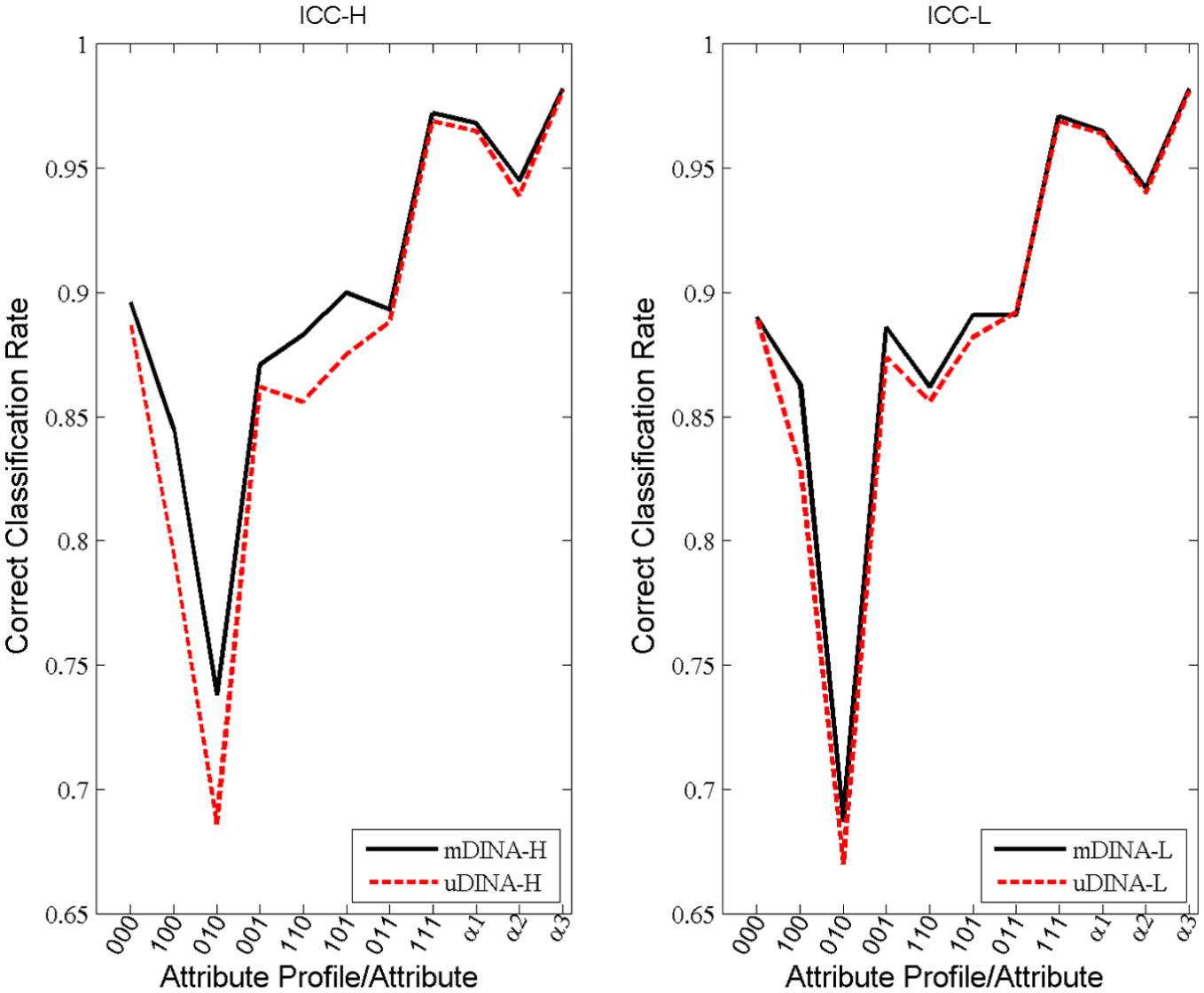
Correct classification rates of the attribute profiles and individual attributes under the ICC-H and ICC-L conditions in the simulation study.

According to the DIC statistic, the data-generating mDINA model was preferred to the uDINA model in 19 to 27 of the 30 replications under the ICC-H condition by an average 30.22 to 98.33 smaller number for the DIC. The mDINA model was preferred 17 to 22 times under the ICC-L condition by an average 10.91 to 49.97 smaller number for the DIC. In general, the longer the test and the larger the number for the schools, the higher the power of the DIC statistic in selecting the true model would be.

Three Attributes Under Condition ICC-0

Under the ICC-0 condition, the uDINA model was the true model and the mDINA model was an unnecessarily complicated model. Both the mDINA and uDINA models recovered the parameters very well, with the bias and RMSE in the second or third decimal places in general. For the estimation of Ω (whose true values were all zero), the mDINA model yielded a bias between 0.007 and 0.098 and RMSE between 0.010 and 0.098. Because the bias and RMSE were very small, there was little difference between the mDINA and uDINA models. In addition, the recovery rates for the attributes and latent profiles under the mDINA model were almost identical to those under the uDINA model. According to the DIC statistic, the uDINA model was preferred in 15 to 20 of the 30 replications by an average of 12.85 to 61.14 smaller in the DIC. In short, it did little harm to fit an unnecessarily complicated model (i.e., the mDINA model) to data without multilevel structures. Detailed results are shown in Table A3 in the online supplement.

The Conditions Under the Five Attributes

The results for ICC-H, ICC-L, and ICC-0 under the conditions of the five attributes are shown in Tables A4 to A6 in the online supplement, respectively. The major findings were the same as those found in the conditions of the three attributes. However, when there were more attributes, the recovery for the individual attributes and attribute profiles became poorer.

An Empirical Study

Data and Analysis

Responses from eighth graders in the United States to the 2003 TIMSS mathematics test were analyzed. The test was designed to measure knowledge on five content domains: algebra, data, geometry, measurement, and number. An example item in the number domain on the relationships among numbers is as follows: “Show that the sum of any two odd numbers is an even number.” For illustrative purposes, the five domains were treated as five binary attributes in this study. The structure of the Q-matrix was not complex because each item measured only one of the five domains. Although the TIMSS test was not designed specifically to diagnose binary attributes, it was used to demonstrate the utilities of CDMs in previous studies (Lee, Park, & Taylan, 2011; Tatsuoka, Corter, & Tatsuoka, 2004).

The data consisted of 50 items and 100 schools (90% were public), which comprised 3,710 students (52% were girls). The original data set consisted of responses to 362 items from 8,912 students and 232 schools; among them there were 88, 52, 57, 57, and 108 items measuring algebra, data, geometry, measurement, and number, respectively. The number of students in each school ranged from 4 to 63 (M = 37.1). There were 12, four, 13, six, and 15 items for the five domains, respectively. Each student completed 1 to 9 (M = 5.88) items, and each item was responded to by 294 to 922 (M = 437.02) students. The data consisted of many missing values that were caused mainly by the matrix-sampling design used in the TIMSS, where a student was administered a subset of items or booklet (Mullis, Martin, Gonzalez, & Chrostowski, 2004). Thus, the data were missing by design and treated as missing at random in this study (Mislevy & Wu, 1996). The authors were particularly interested in the following three questions:

What was the school effect as indicated by the ICC?

What were the correlations among the five attributes?

What were the gender (girl = 0, boy = 1) and school type (private = 0, public = 1) differences in the five attributes?

Five models were fit to the data: (a) the uDINA model (which served as the baseline model), (b) the mDINA model, (c) the mDINA model with gender as a student-level covariate (denoted as mDINA-G), (d) the mDINA model with school type as a school-level covariate (denoted as mDINA-S), and (e) the mDINA model with gender as a student-level covariate and school type as a school-level covariate (denoted as mDINA-GS). The priors were specified as those in the simulation study. The MCMC procedure had a run length of 20,000 iterations with a burn-in length of 5,000 iterations. It took approximately 9 computer hours for the most complicated mDINA-GS model. The five models were compared according to the DIC values.

The posterior predictive model checking (PPMC; Gelman, Meng, & Stern, 1996) method was used to examine the fit of the models. This study focused on the person- and item-level fit statistics. For the person-level fit statistics, the number-correct score was used for each student, whose range was from 0 to 9. For the item-level fit, the percentage of correct answers was computed. The differences of the two statistics between the observed and replicated data were examined.

Results

The DIC values were 21,740 for mDINA-GS, 22,725 for mDINA-G, 22,745 for mDINA-S, 22,853 for mDINA, and 24,152 for uDINA. The mDINA-GS model had the smallest DIC value (JAGS code is shown in the online supplement). For PPMC results, both statistics indicated a good fit for the mDINA-GS model. The results are available upon request. As the mDINA model had a better fit than the uDINA model, a multilevel data structure was found. According to the mDINA model without any predictor, the ICC values were 0.50, 0.39, 0.41, 0.38, and 0.42 for the five attributes, respectively, and the design effect values were 18.92, 15.06, 15.89, 14.71, and 16.06, respectively, indicating a strong school effect. The results were consistent with previous findings, which found substantial between-school variations (ICC = 0.48) among eighth graders in the United States for the 2003 TIMSS mathematics test (Z. Wang, Osterlind, & Bergin, 2012).

Table 1 shows the parameter estimates and the standard errors for the regression coefficients, and the student-level and school-level variance–covariance matrices in the mDINA-GS model. The g- and s-parameter estimates, not listed due to space constraints, were between 0.01 and 0.42. The Wald test on the regression coefficients of gender for the five attributes suggested that boys had a statistically higher mastery level than girls in the measurement and number attributes, which was consistent with the findings in the TIMSS 2003 mathematics report (Mullis et al., 2004). The Wald test on the regression coefficients of school type for the five attributes indicated that private schools had a statistically higher mastery than public schools on algebra and number attributes. The school-type difference was also consistent with previous studies (Rutkowski & Rutkowski, 2010). The five attributes were moderately correlated in a range of 0.46 (between Attributes 1 and 4) and 0.63 (between Attributes 1 and 3).

Table 1.

Parameter Estimates Under the mDINA-GS in the Empirical Example With the LCV and MBD Approaches.

	LCV		MBD
Parameter	Estimate	Standard Error	Estimate	Standard Error
υ₀₀₁	0.548	0.248	0.472	0.558
υ₀₀₂	−0.477	0.225	−0.688	0.524
υ₀₀₃	0.353	0.195	0.185	0.496
υ₀₀₄	−0.820	0.210	−0.216	0.658
υ₀₀₅	0.258	0.231	−0.330	0.737
υ₁₀₁	−0.328	0.117	−0.628	0.180
υ₁₀₂	0.078	0.131	−0.027	0.337
υ₁₀₃	−0.099	0.071	−0.184	0.187
υ₁₀₄	0.428	0.129	0.534	0.254
υ₁₀₅	0.161	0.074	0.351	0.200
υ₀₁₁	−0.350	0.168	−0.211	0.284
υ₀₁₂	0.147	0.254	0.775	0.328
υ₀₁₃	−0.169	0.137	0.336	0.274
υ₀₁₄	−0.016	0.199	−0.235	0.322
υ₀₁₅	−0.442	0.120	−0.325	0.207
σ₁₂	0.604	0.026	0.480	0.033
σ₁₃	0.634	0.016	0.506	0.025
σ₁₄	0.456	0.027	0.401	0.029
σ₁₅	0.617	0.024	0.459	0.022
σ₂₃	0.613	0.028	0.476	0.032
σ₂₄	0.469	0.029	0.444	0.032
σ₂₅	0.559	0.028	0.470	0.031
σ₃₄	0.612	0.030	0.430	0.029
σ₃₅	0.523	0.024	0.470	0.028
σ₄₅	0.561	0.027	0.475	0.043
ω₁₁	0.986	0.140	3.239	0.241
ω₁₂	0.661	0.158	2.779	0.269
ω₁₃	0.707	0.171	2.897	0.299
ω₁₄	0.639	0.183	2.752	0.261
ω₁₅	0.726	0.206	2.756	0.251
ω₂₂	0.638	0.151	2.862	0.269
ω₂₃	0.555	0.140	2.711	0.243
ω₂₄	0.497	0.120	2.627	0.234
ω₂₅	0.572	0.132	2.691	0.216
ω₃₃	0.702	0.198	3.017	0.270
ω₃₄	0.508	0.142	2.680	0.256
ω₃₅	0.606	0.141	2.758	0.207
ω₄₄	0.612	0.162	2.797	0.235
ω₄₅	0.552	0.130	2.704	0.239
ω₅₅	0.716	0.176	3.002	0.271

Note.υ₀₀₁ to υ₀₀₅ are the intercepts for the five attributes (algebra, data, geometry, measurement, and number); υ₁₀₁ to υ₁₀₅ are the regression coefficients of gender (boy = 1) for the five attributes; υ₀₁₁ to υ₀₁₅ are the regression coefficients of school type (public = 1) for the five attributes; σ is the student-level covariance; ω is the school-level covariance. The parameter estimates in the two approaches are not directly comparable because they are not on the same metric. mDINA-GS = multilevel deterministic input, noisy, and gate model with gender as a student-level covariate and school type as a school-level covariate; LCV = latent continuous variable; MBD = multivariate Bernoulli distribution.

The classification of examinees was taken from the best-fitting mDINA-GS model as a gold standard and Cohen’s kappa coefficient was computed to examine the agreement in the attribute and profile classifications between the mDINA-GS and the uDINA models. The coefficients were between 0.64 and 0.73 for the five attributes and the coefficient was 0.38 for the profiles, indicating a moderate agreement (Landis & Koch, 1977). Thus, ignoring multilevel data structures would affect the classification of attributes and profiles seriously.

For illustrative purposes, the MBD approach also was adopted (the JAGS code is shown in the online appendix). When fitting the model with student-level and school-level predictors, it took approximately 6 hr to converge in JAGS. The resulting DIC was 23,662, which was larger than that of the LCV approach (21,740). According to Equation 8, the MBD approach yielded an ICC of 0.25, 0.28, 0.25, 0.24, and 0.27 for the five attributes, respectively. Although these values were not the same as those from the LCV approach, they all suggested large school effects on the attributes. As expected, the estimates for g- and s-parameter from the two approaches were almost identical, with correlations around 0.99. The two approaches yielded substantial agreement in classification, with Cohen’s kappa coefficients between 0.73 and 0.83 for the five individual attributes and 0.80 for the attribute profiles. The other parameter estimates are shown in Table 1. Note that, although they were not on the same metric, the estimation patterns were very similar. For example, both approaches found that boys had a statistically higher mastery level in the measurement and number attributes and that Attribute 1 (algebra) and Attribute 3 (geometry) had the highest positive correlation.

An additional simulation study that mimicked the design of the empirical example was conducted to evaluate the parameter recovery for the LCV and MBD approaches. The item estimates, person estimates, and regression coefficients in Table 1 under each approach were used as generating values. The data-generating model was fit to the data using JAGS with priors and settings similar to those in the empirical example. Thirty replications were conducted. The bias and RMSE in the estimates were computed. The parameter recovery in both approaches was found to be satisfactory. The results are provided in the online supplement.

Conclusion and Discussion

Two-staged or multi-staged sampling has become popular, especially in large-scale assessments. Such a sampling creates multilevel data structures. The consequences of ignoring multilevel structures have been well documented in the literature, and a variety of multilevel linear models and IRT models have been developed. Most existing CDMs are unilevel and become infeasible for multilevel data. This study developed a new class of multilevel CDMs in which the general LCDM was used as the item-level model and the LCV and MBD approaches were proposed to formulate the Level 1 and Level 2 models. Covariates can be incorporated directly into each level, and their effects on attribute mastery can be conveniently estimated. The standard errors of the covariates can be estimated accurately, and the accuracy of attributes and profiles classification for individuals can be improved.

A series of simulations were conducted to evaluate the parameter recovery of the new multilevel CDMs and the consequences of ignoring multilevel structures on parameter estimation. Due to high dimensionality, Bayesian methods with MCMC algorithms were adopted. For simplicity, the mDINA and uDINA models were used for demonstration. It was found that, when the data-generating mDINA model was fit to mDINA data, all parameters were recovered fairly well. The longer the test was and the larger the number of schools were, the better the parameter recovery. When the mDINA model was fit to data generated from the uDINA model, there was little harm in parameter estimation, and the estimates for the school-level variance–covariance matrix were very close to zero.

On the contrary, when the uDINA model was fitted to mDINA data (and the multilevel structures were ignored), the estimates for the item parameters and their standard errors were not affected, but the standard errors of the student-level covariates were underestimated, which is consistent with the findings in multilevel linear models or IRT models. The estimates for the student-level covariates were poor, especially when the ICC was high, because the variance of the student level was constrained to be 1 for model identification. These results were different from those in multilevel linear models or IRT models, where it was found that the variance of the ignored level (e.g., school level) is redistributed to the adjacent level (e.g., student level) and the variance of the student level is estimated inaccurately. Finally, ignoring multilevel structures also resulted in poorer recovery of the latent profiles of individuals. As a conclusion, when there is a doubt about multilevel effects, fitting both unilevel and multilevel CDMs and comparing their differences are recommended.

The empirical example of the 2003 TIMSS mathematics test shows that boys and private schools had a higher percentage of mastering the attributes than girls and public schools, and the five attributes were moderately correlated. It will be valuable for future studies to apply the multilevel CDMs to real tests to investigate the effects of student-level and/or school-level covariates on attribute mastery when data have multilevel structures.

The LCV and MBD approaches yielded nearly identical estimates for item parameters, substantial agreement in attribute and profile classifications, and similar patterns for the regression coefficients of covariates and correlations among latent variables. The two approaches have strengths and limitations. The LCV approach is preferred because it is easier to implement with existing computer programs.

This study is not without limitations. Although the new models were developed using the LCDM (Henson et al., 2009) as the item-level model, they can be applied to other general CDMs, such as the GDM (von Davier, 2010) and G-DINA model (de la Torre, 2011). For simplicity, the mDINA model was used as an example in this study; however, formulation of other multilevel CDMs (e.g., the multilevel DINO and multilevel fusion models) are straightforward and can be used for future studies.

Item parameters in CDMs (e.g., the slip parameter and guessing parameter in the DINA model) often are treated as fixed effects, indicating that they are identical across persons. This assumption may be too strict in some situations. For example, the levels of slipping may depend on examinee motivation, and the levels of guessing may be related to the examinee’s ability. If so, it would be more flexible to treat the item parameters as random effects. When appropriate, the random-effect approach proposed by Huang and Wang (2014) can be incorporated in multilevel CDMs. In addition, this study focused on the random-intercept multilevel CDMs. It is valuable for future studies to investigate random-slope multilevel CDMs where the cross-level interactions among predictors at different levels are possible (Hox, 2010).

Supplemental Material

4online_supplements.R3_v2 – Supplemental material for Multilevel Modeling of Cognitive Diagnostic Assessment: The Multilevel DINA Example

Supplemental material, 4online_supplements.R3_v2 for Multilevel Modeling of Cognitive Diagnostic Assessment: The Multilevel DINA Example by Wen-ChungWang and Xue-Lan Qiu in Applied Psychological Measurement

Footnotes

Acknowledgements

The authors thank Dr. Jimmy de la Torre and two anonymous reviewers for their constructive comments on earlier drafts of this article.

Declaration of Conflicting Interests

The author(s) declared no potential conflicts of interest with respect to the research, authorship, and/or publication of this article.

Funding

The author(s) disclosed receipt of the following financial support for the research, authorship, and/or publication of this article: This study was supported by General Research Fund, Research Grants Council (No. 18604515).

ORCID iD

Wen-Chung Wang

Supplementary Material

Supplemental material is available for this article online.

References

Asparouhov

Muthén

(2010). Bayesian analysis using Mplus: Technical implementation: Technical appendix. Los Angeles, CA: Muthén & Muthén.

Ayers

Rabe-Hesketh

Nugent

(2013). Incorporating student covariates in cognitive diagnosis models. Journal of Classification, 30, 195-224.

Chang

Y.-W.

Tsai

R.-C.

Hsu

N.-J.

(2014). A speeded item response model: Leave the harder till later. Psychometrika, 79, 255-274.

Dai

Ding

Wahba

(2013). Multivariate Bernoulli distribution. Bernoulli, 19, 1465-1483.

Daniels

M. J.

Kass

R. E.

(1999). Nonconjugate Bayesian estimation of covariance matrices and its use in hierarchical models. Journal of the American Statistical Association, 94, 1254-1263.

de Boeck

Wilson

(Eds.). (2004). Explanatory item response models: A generalized linear and nonlinear approach. New York, NY: Springer.

de la Torre

(2011). The generalized DINA model framework. Psychometrika, 76, 179-199.

de la Torre

Douglas

J. A.

(2004). Higher-order latent trait models for cognitive diagnosis. Psychometrika, 69, 333-353.

Entink

R. H. K.

Fox

J. P.

van der Linden

W. J.

(2009). A multivariate multilevel approach to the modeling of accuracy and speed of test takers. Psychometrika, 74, 21-48.

10.

Fox

J.-P.

Glas

C. A. W.

(2001). Bayesian estimation of a multilevel IRT model using Gibbs sampling. Psychometrika, 66, 271-288.

11.

Gelman

Meng

X.-L.

Stern

H. S.

(1996). Posterior predictive assessment of model fitness via realized discrepancies. Statistical Sinica, 6, 733-807.

12.

Goldstein

(2010). Multilevel statistical models (4th ed.). London, England: Arnold.

13.

Hartz

S. M.

(2002). A Bayesian framework for the unified model for assessing cognitive abilities: Blending theory with practicality (Unpublished doctoral dissertation). University of Illinois at Urbana–Champaign.

14.

Henson

Templin

Willse

(2009). Defining a family of cognitive diagnosis models using log-linear models with latent variables. Psychometrika, 74, 191-201.

15.

Hox

J. J.

(2010). Multilevel analysis: Techniques and applications (2nd ed.). New York, NY: Routledge.

16.

Huang

H.-Y.

Wang

W.-C.

(2014). The random-effect DINA model. Journal of Educational Measurement, 51, 75-97.

17.

Junker

B. W.

Sijtsma

(2001). Cognitive assessment models with few assumptions, and connections with nonparametric item response theory. Applied Psychological Measurement, 25, 258-272.

18.

Karlis

Xekalaki

(2003). Choosing initial values for the EM algorithm for finite mixtures. Computational Statistics & Data Analysis, 41, 577-590.

19.

Landis

J. R.

Koch

G. G.

(1977). The measurement of observer agreement for categorical data. Biometrics, 33, 159-174.

20.

Lee

Y.-S.

Park

Y. S.

Taylan

(2011). A cognitive diagnostic modeling of attribute mastery in Massachusetts, Minnesota, and the U.S. national sample using the TIMSS 2007. International Journal of Testing, 11, 144-177.

21.

Liu

Daniels

M. J.

(2006). A new algorithm for simulating a correlation matrix based on parameter expansion and reparameterization. Journal of Computational and Graphical Statistics, 15, 897-914.

22.

Mislevy

R. J.

P. K.

(1996). Missing responses and IRT ability estimation: Omits, choice, time limits, and adaptive testing (Research Report No. RR-96-30-ONR). Princeton, NJ: Educational Testing Service.

23.

Mullis

I. V. S.

Martin

M. O.

Gonzalez

E. J.

Chrostowski

S. J.

(2004). TIMSS 2003: International mathematics report. Boston, MA: TIMSS & PIRLS International Study Center, Boston College.

24.

Pearson

(1900). Mathematical contributions to the theory of evolution, VII: On the correlation of characters not quantitatively measurable. Philosophical Transactions of the Royal Society of London. Series A, 19, 51-147.

25.

Plummer

(2003, March). JAGS: A program for analysis of Bayesian graphical models using Gibbs sampling. Paper presented at the Proceedings of the 3rd International Workshop on Distributed Statistical Computing, Vienna, Austria.

26.

Plummer

Best

Cowles

Vines

(2006). CODA: Convergence diagnosis and output analysis for MCMC. R News, 6, 7-11.

27.

Rupp

A. A.

Templin

J. L.

Henson

R. A.

(2010). Diagnostic assessment: Theory, methods, and application. New York, NY: Guilford Press.

28.

Rutkowski

(2010). Private and public education: A cross-national exploration with TIMSS 2003 (Working Paper No. 192). Retrieved from http://ncspe.tc.columbia.edu/working-papers/OP192.pdf

29.

Spiegelhalter

D. J.

Best

N. G.

Carlin

B. P.

van der Linden

(2002). Bayesian measures of model complexity and fit. Journal of the Royal Statistical Society, Series B, 64, 583-640.

30.

Steenbergen

M. R.

Jones

B. S.

(2002). Modeling multilevel data structures. American Journal of Political Science, 46, 218-237.

31.

Tatsuoka

K. K.

Corter

J. E.

Tatsuoka

(2004). Patterns of diagnosed mathematical content and process skills in TIMSS-R across a sample of 20 countries. American Educational Research Journal, 41, 901-926.

32.

Templin

J. L.

Henson

R. A.

(2006). Measurement of psychological disorders using cognitive diagnosis models. Psychological Methods, 11, 287-305.

33.

von Davier

. (2010). Hierarchical mixtures of diagnostic models. Psychology Science Quarterly, 52, 8-28.

34.

Wang

W.-C.

Qiu

X.-L.

(2013). A multidimensional and multilevel extension of a random-effect approach to subjective judgment in rating scales. Multivariate Behavioral Research, 48, 398-427.

35.

Wang

Osterlind

S. J.

Bergin

D. A.

(2012). Building mathematics achievement models in four countries using TIMSS 2003. International Journal of Science and Mathematics Education, 20, 1215-1242.

Supplementary Material

Please find the following supplemental material available below.

For Open Access articles published under a Creative Commons License, all supplemental material carries the same license as the article it is associated with.

For non-Open Access articles published, all supplemental material carries a non-exclusive license, and permission requests for re-use of supplemental material or any part of supplemental material shall be sent directly to the copyright owner as specified in the copyright notice associated with the article.

0.00 MB

1.43 MB