Answer Similarity Analysis at the Group Level

Abstract

Answer similarity indices were developed to detect pairs of test takers who may have worked together on an exam or instances in which one test taker copied from another. For any pair of test takers, an answer similarity index can be used to estimate the probability that the pair would exhibit the observed response similarity or a greater degree of similarity under the assumption that the test takers worked independently. To identify groups of test takers with unusually similar response patterns, Wollack and Maynes suggested conducting cluster analysis using probabilities obtained from an answer similarity index as measures of distance. However, interpretation of results at the cluster level can be challenging because the method is sensitive to the choice of clustering procedure and only enables probabilistic statements about pairwise relationships. This article addresses these challenges by presenting a statistical test that can be applied to clusters of examinees rather than pairs. The method is illustrated with both simulated and real data.

Keywords

test security item response theory test collusion

To establish validity of test scores, investigators typically assume that examinees respond to exam items independently using their knowledge, skills, or abilities related to the construct being measured. This assumption can be violated in a variety of ways, including examinees copying from each other or responding to test items using preknowledge of live exam content. Statistical methods to detect examinees who do not respond to exam items independently originally focused on analysis of pairs of examinees, reflecting the assumption that anomalous response patterns could occur due to answer copying. However, as testing programs have moved into computer-based testing and as digital communication devices (e.g., cell phones with cameras) have become ubiquitous, the problem of identifying anomalous responses due to inappropriate testing behaviors has become much more complex. Examinees can more easily access and more widely share test content using a variety of strategies, and nonindependent test taking does not have to be limited to pairs or small groups with some connection to each other. For example, Haberman and Lee (2017) describe the problem of key sharing, which may involve examinees from various test locations who have no connection to each other except access to the same distributed key. As the ways in which test takers may have prior knowledge to the same subset of exam content or the same shared key become increasingly complex, statistical methods to identify group-level collusion are needed.

Wollack and Maynes (2017) introduced a method to detect group level collusion by combining the use of an answer similarity index and cluster analysis. Answer similarity indices (see, e.g., van der Linden and Sotaridona’s (2006) generalized binomial test (GBT) and Maynes’ (2014)M4 statistic) were developed to detect unusually high numbers of matching responses between pairs of examinees to identify pairs who may have worked together on an exam, or instances in which one examinee copied from another examinee. For any pair of examinees, an answer similarity index is used to estimate the probability that the pair would exhibit the observed response similarity or a greater degree of similarity under the assumption that the test takers worked independently. Such probabilities can be calculated for every pair of examinees and used to create a distance matrix for clustering.

The distance matrix is a lower triangular matrix in which the entry for examinees i and j (for i > j) in row i and column j is the p-value (or some transformed version of the p-value, as described by Wollack & Maynes, 2017) calculated using an answer similarity index. The user needs to specify a threshold δ that corresponds to the clustering criterion. For example, if δ = 0.001 (in the p-value metric) and nearest-neighbor clustering is used, examinees will be included in a cluster if the pairwise answer similarity p-value with one or more examinees in the cluster is less than 0.001. Wollack and Maynes recommend employing a multiple comparisons correction due to the similarity index being computed N−1 times for the same examinee. They chose to implement the correction at the examinee level for α = 0.05, in which the alpha level is divided by (N−1)/2. While Wollack and Maynes showed how answer similarity analysis and cluster analysis can be used together with the M4 similarity index and nearest-neighbor clustering, many choices exist for both the similarity index and clustering method that could be employed. See Gocer Sahin and Wollack (2018) for an evaluation of the impact of using various clustering methods (i.e., nearest-neighbor, complete linkage, average linkage, centroid, and Ward) using the GBT similarity index.

Several aspects of the general methodology employed by Wollack and Maynes (i.e., forming clusters of examinees based on pairwise similarity analyses; henceforth referred to as the WM method) introduce difficulties in interpretation of results. It is important to note that these difficulties are not limited to the specific choice of similarity index, clustering method, or clustering threshold described by Wollack and Maynes (2017). First, the probabilistic statements are based on pairwise relationships, not cluster relationships. Second, it is not necessarily true that candidates identified in the same cluster will have response patterns that are very similar to each other. The choice of clustering method, the clustering threshold, and the number of pairwise comparisons conducted will influence how heterogeneous a cluster may be in terms of response similarity. For example, Belov and Wollack (2018) note that nearest-neighbor classification can produce long-chained clusters (Blashfield & Aldenderfer, 1988) in which many distinct smaller groups or individuals are linked together by weak connections, potentially leading to clusters in which many of the elements in the cluster are dissimilar. Wollack and Maynes (2017) also presented results of simulations showing that the method can produce clusters consisting of individuals from more than one simulated collusion group along with examinees with no simulated collusion.

While the WM method is promising to detect groups of individuals who may have colluded or had preknowledge of the same subset of items, interpretation of the results would be greatly aided by a method that analyzes the response patterns of all of the examinees in a cluster. This article introduces such a method by presenting a statistical test to estimate the probability that the minimum number of pairwise matching responses in a cluster is the observed minimum or greater under the assumption that all examinees in the cluster are working independently. The method is illustrated using simulated data and real data from an information technology (IT) certification exam that experienced known compromise.

Overview of the Generalized Binomial Answer Similarity Index

As the methodology introduced in this article will use the generalized binomial answer similarity index (GBT index) (van der Linden & Sotaridona, 2006), a brief overview of the index is provided. Comprehensive reviews of answer similarity analysis can be found in Maynes (2017) and Zopluoglu (2017). The GBT index can be calculated for any pair of examinees and provides an estimate of the probability that those examinees would exhibit the observed number of matching responses or greater given their individual ability levels and the item parameters. The GBT will be used rather than M4 as described in the Wollack and Maynes (2017) because the method presented in this article relies on the normal approximation of the generalized binomial distribution (described in more detail below).

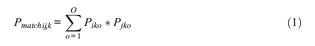
The probability of examinees i and j matching on item k is calculated as

P_{m a t c h i j, k} = \sum_{o = 1}^{O} P_{i k o} * P_{j k o}

(1)

where $O$ is the number of response options and $P_{iko}$ and $P_{jko}$ are probabilities of examinees i and j selecting response option o, determined using an appropriate item response theory (IRT) model. The probability of observing exactly m matches on $K$ items is calculated as

f_{ij, K} (m) = \sum_{c = 1}^{{}_{K}^{.}{C_{m}}} (Π_{k = 1}^{K} {({P_{match}}_{ij, k})}^{u_{k_c}} * {(1 - {P_{match}}_{ij, k})}^{1 - u_{k_c}})

(2)

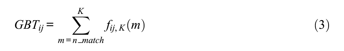
where, for each possible combination $c$ of $m$ matches on $K$ items, $u_{k_c}$ is equal to 1 if the two examinees’ responses match for item k, and 0 if the two examinees’ responses do not match for the particular combination. For example, the number of combinations in which examinees i and j could match on exactly 2 of 60 items is ${}_{60}^{.}{C_{2}} = 60! / 2! 58! = 1, 770$ . For the combination c in which the examinees matched on the first two items, $u_{k_c} = {\begin{matrix} 1, k \in {1, 2} \\ 0, k \in {3, \dots, 60} \end{matrix} .$ Note that the values $u_{k_c}$ are not dependent on the actual matches in the observed response patterns of examinees i and j.

The GBT index is calculated by summing the values of $f_{ij, K} (m)$ which are part of the upper tail of the generalized binomial distribution.

GB T_{ij} = \sum_{m = n_match}^{K} f_{ij, K} (m)

(3)

where $n_match$ is the number of observed matches. van der Linden and Sotaridona (2006) note that $f_{ij, K} (m)$ can be calculated using the recursive procedure by Lord and Wingersky (1984), which becomes necessary when the number of combinations of $m$ matches on $K$ items is large. For a cluster consisting of n_c examinees, $(n_{c} * (n_{c} - 1)) / 2$ sampling distributions of the number of matching responses can be shown—one for each pair of examinees.

It is important to note that counts of matching responses will differ depending on the choice of IRT model. For example, if the Rasch (1960/1980) model is employed, two examinees who choose different distractors of an item would be described as having matching responses for that item because the Rasch model only estimates two probabilities of response per item (i.e., one for a correct response and one for an incorrect response), and both distractor choices are incorrect; however, if the nominal response model (Bock, 1972) is employed, the examinees will not be described as having matching responses because a different probability of response is estimated for each distractor. Discussion on the implications of IRT model choice is included in the section describing the simulation.

Method

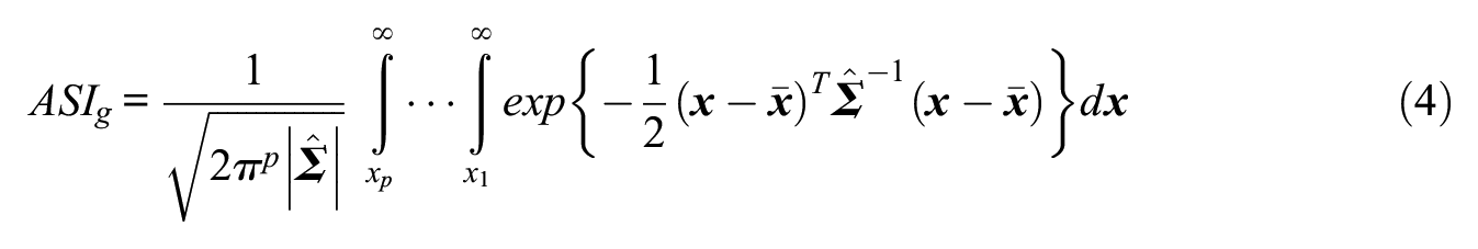
The new statistic presented below, an answer similarity index at the group level (ASI_g), is used to estimate the probability that the minimum number of pairwise matching responses in a cluster is the observed minimum or greater under the assumption that all examinees in the cluster are working independently. To conduct a statistical test based on the response patterns of an entire cluster of examinees rather than simply a pair of examinees, one needs to establish a group-level statistic with a known sampling distribution. In pairwise answer similarity analysis, the number of matching responses among the pair of examinees is often the statistic of interest. For group-level similarity analysis, we will use the minimum number of pairwise matching responses among a group of examinees, which we will refer to as M_min. The M_min is chosen as the test statistic because it generally will represent the weakest connection among a pair of examinees in a cluster (and, even if it does not, the weakest connection will still be included in the cumulative probability, M_min or greater). In addition, the test will be inherently conservative in describing the unusualness of the response patterns in a cluster when there is variation in the number of matching pairwise responses among examinees in the cluster. This is in contrast to other potential test statistics that could be employed such as the mean of the number of matched responses for a cluster.

To calculate ASI_g for a group of examinees, we will rely on the fact that the number of matching responses for each pair of examinees i and j is a discrete random variable M_ij, the distribution of which can be approximated by a normal distribution due to the Liapounov theorem (i.e., the central limit theorem for independent nonidentical random variables) (Lehmann, 1999, sect. 2.7; van der Linden & Sotaridona, 2006). The mean of each M_ij is estimated by $\sum_{k = 1}^{K} ({P_{match}}_{ij, k})$ , and the variance is estimated by $\sum_{k = 1}^{K} ({P_{match}}_{ij, k}) * (1 - {P_{match}}_{ij, k})$ . It is important to note that these random variables M_ij are not mutually independent because independence would imply, for example, that in a cluster of three examinees, examinee 1 could have a different response pattern for pair 1,2 than for pair 1,3. Thus, ASI_g needs to effectively constrain the response pattern for each examinee in the cluster to be the same for each pair where the examinee appears. This constraint introduces challenges to calculating the exact probability of a given minimum number of matching responses, even for small clusters and modest test lengths, which is the reason ASI_g uses the normal approximation of the compound binomial to approximate the distribution of the number of matching responses for each pair of examinees.

Assume the joint distribution of the $p = (n_{c} * (n_{c} - 1)) / 2$ random variables M_ij for $n_{c}$ examinees in a cluster is distributed as

M_{ij} ~ N (μ_{M}, Σ_{M}),

where $μ_{M} = [\begin{matrix} μ_{M_{12}} \\ ⋮ \\ μ_{M_{(n - 1) n}} \end{matrix}]$ and $Σ_{M} = [\begin{matrix} \begin{matrix} σ_{M_{12}}^{2} & σ_{M_{12}, M_{13}} \\ σ_{M_{12}, M_{13}} & σ_{M_{13}}^{2} \end{matrix} \\ \begin{matrix} ⋮ & \dots \\ σ_{M_{12}, M_{(n - 1) n}} & \dots \end{matrix} \end{matrix} \begin{matrix} \begin{matrix} \dots & σ_{M_{12}, M_{(n - 1) n}} \\ \dots & σ_{M_{13}, M_{(n - 1) n}} \end{matrix} \\ \begin{matrix} ⋱ & ⋮ \\ \dots & σ_{M_{(n - 1) n}}^{2} \end{matrix} \end{matrix}]$ .

ASI_g can be computed by integrating the multivariate normal density function defined by the above mean vector and covariance matrix:

AS I_{g} = \frac{1}{\sqrt{2 π^{p} | \hat{Σ} |}} \int_{x_{p}}^{\infty} \dots \int_{x_{1}}^{\infty} \exp {- \frac{1}{2} {(x - \bar{x})}^{T} {\hat{Σ}}^{- 1} (x - \bar{x})} d x

(4)

The vector x contains p entries of M_min, subtracting 0.5 for Yates’ (1934) continuity correction. The means in $\bar{x}$ and the variances in $\sum^{^}$ are the means and variances of the normal approximations of each M_ij, as described above. The covariances in $\sum^{^}$ are calculated using a Monte Carlo method, where a large number of replications of n_c×K response data matrices (where n_c is the number of examinees in the cluster, and K is the number of items) are generated using estimated examinee abilities and item parameters. These simulated data sets represent other possible response patterns than those observed for a given set of items and examinee parameters. For each examinee pair in each simulated response matrix, the number of matching responses is calculated. Using these values, for each dependent pair of examinee pairs (e.g., examinee pair 1,2 and examinee pair 1,3), the covariance of the number of matching responses is calculated. Covariances for each independent pair of examinee pairs (e.g., examinee pair 1,2 and examinee pair 3,4) are logically equal to zero. In all instances in this article, 100,000 replications of response matrices were used, although some exploratory simulations indicated that as few as 1,000 replications seemed to function similarly to higher numbers of replications.

The assumption of multivariate normality is not exactly satisfied for two reasons. First, a normal approximation is used for each individual M_ij to approximate a discrete distribution. van der Linden and Sotaridona (2006) showed that the normal approximation does not work as well for small numbers of items and examinee pairs with very different ability levels. Second, although each distribution of each M_ij is approximately normal, the joint distribution of dependent normally distributed random variables is not necessarily multivariate normal. While multivariate normality holds if and only if each linear combination of its components is univariate normal (Johnson & Wichern, 1998), one can check whether the multivariate normality assumption is reasonable by assessing the normality of each M_ij and by comparing the density of squared Mahalanobis distances to a chi-square distribution with $p$ degrees of freedom (Andrews et al., 1973).

Simulation

Assessing spurious clusters

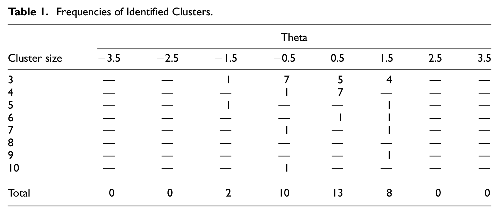
The simulation study in this article was designed to evaluate how ASI_g performs across the range of examinee ability under conditions in which the WM method would likely produce spurious clusters. Thus, no collusion was simulated, and ASI_g will be evaluated in terms of how well it helps identify any clusters from the WM method as spurious and how closely the probability distribution of M_min calculated using ASI_g aligns with an empirically derived distribution. For each of eight values of examinee ability across the ability spectrum (i.e., θ = −3.5, −2.5, −1.5, −0.5, 0.5, 1.5, 2.5, and 3.5), 500 response vectors were generated assuming that examinees’ responses to a 60-item test (where item difficulties were randomly drawn from a $N (0, 1)$ distribution) fit a Rasch model. These specifications were chosen for consistency with the real data example. For each level of examinee ability, the WM method was carried out using the GBT as the answer similarity index and nearest-neighbor clustering as the clustering method.

GBT calculations assumed examinee responses followed a Rasch model; thus matching incorrect responses were treated as matching regardless of potentially different distractor choices. The Rasch model was used here because the exam program that supplied the real data uses the Rasch model operationally for scoring, and it is a common practice in the field of IT security to use the same IRT model for scoring and security analyses. In addition, the real data example is constrained by sample size, so it was not possible to conduct analyses using the nominal response model to take distractor choice into account. However, as it is not common practice in other areas of educational measurement to ignore distractor choice in investigations of answer similarity, it is worth discussing the implications of doing so here. If two examinees generally match on the distractors of incorrect responses, yet the IRT model does not take distractor choice into account, the estimated probability of the unusualness of the number of matching responses will likely be an overestimate of the true probability. Zopluoglu’s (2017) simulation study that compared the performance of various answer similarity indices showed that the empirical type-I error rates of the GBT were well controlled for both dichotomous and nominal response outcomes, but power was lower for dichotomous outcomes. When feasible, practitioners should empirically examine the impact of using an IRT model that considers distractor choice versus one that does not to help establish the most appropriate analysis procedures and to ensure appropriate inferences are made in all situations (e.g., when pairs of examinees have large numbers of matching incorrect responses with different distractors).

Within each ability level, the GBT was conducted for each pair of examinees for a total of 124,750 GBT tests per ability level. The choice to separate the analysis by ability level was made for two reasons. First, examinees of the same ability level that are working independently are more likely to have higher levels of matching responses than those of different ability levels, increasing the opportunity for spurious flags. Second, for a given set of item parameters, the center and spread of the distribution of matching responses for two examinees with equal ability is expected to differ across different ability levels. In addition, how well the normal approximation of the binomial approximates the exact distribution is also expected to vary across the ability spectrum. The separate analyses were done to isolate these differences.

For each level of θ used for the simulations, Figures A1 and A2 in Supplemental Appendix A show the exact probability distribution of the number of matching responses for a pair of examinees (used in the GBT) and the corresponding normal approximation to illustrate the variability in the distributions across the θ range. Figure A1 shows the distributions for pairs of examinees with the same ability level (mimicking the design of the simulation study in this article), and Figure A2 shows the distributions for pairs of examinees with different ability levels. One can see that using the normal approximation appears to be warranted for a test of this length with the given item parameters both for pairs of examinees with similar and differing ability levels. However, it is clear from visual inspection that the approximation is better for less extreme values of θ.

GBT calculations were conducted using a version of the CopyDetect R package (Zopluoglu, 2018) modified by the author to allow for fixing item and person parameters to values estimated externally. Item parameters were fixed to the generating parameters, and person parameters were estimated using maximum likelihood estimation with the cacIRT R package (Lathrop, 2015). Nearest-neighbor clustering was conducted using the stats R package (R Core Team, 2018). The multivariate normal integration required for ASI_g was conducted using the randomized Quasi-Monte-Carlo procedure (Genz, 1992) implemented in the mvtnorm R package (Genz et al., 2018).

Across all levels of θ, 105 total clusters (including clusters of only two examinees) were identified using the WM methodology with a flagging criterion for a pair of examinees of 0.001. Using the nearest-neighbor clustering method with a clustering threshold of $δ = 0.001$ , any examinee flagged with another examinee in a cluster with a GBTp-value less than 0.001 was included in the cluster. The fairly liberal flagging criterion and clustering threshold (for a test security context) were chosen to ensure that a variety of spurious clusters would be identified. No Bonferroni adjustments were made to control for multiple comparisons for the same reason. Of the 105 identified clusters, 33 consisted of more than two examinees. The 33 clusters of three or more examinees are considered in the results because the GBT is essentially the exact probability that the ASI_g approximates for clusters of size 2 (i.e., pairs of examinees). Frequencies of identified clusters of sizes 3 to 10 are shown in Table 1. Note that no clusters of three or more examinees were flagged for θ levels −3.5, −2.5, 2.5, and 3.5.

Table 1.

Frequencies of Identified Clusters.

	Theta
Cluster size	−3.5	−2.5	−1.5	−0.5	0.5	1.5	2.5	3.5
3	—	—	1	7	5	4	—	—
4	—	—	—	1	7	—	—	—
5	—	—	1	—	—	1	—	—
6	—	—	—	—	1	1	—	—
7	—	—	—	1	—	1	—	—
8	—	—	—	—	—	—	—	—
9	—	—	—	—	—	1	—	—
10	—	—	—	1	—	—	—	—

Total	0	0	2	10	13	8	0	0

To assess the assumption that the joint distribution of all M_ij’s is multivariate normal, Supplemental Appendix B shows the density of squared Mahalanobis distances calculated using the simulated response data used to estimate the covariances of the M_ij’s (i.e., 100,000 $n_{c}$ × $K$ response data matrices) compared to a chi-square distribution with $p$ degrees of freedom. The squared Mahalanobis distance was computed for each of the 100,000 simulated response data matrices. The density of the squared Mahalanobis distance is nearly indistinguishable from the appropriate chi-square distribution for each of the example clusters shown in Supplemental Appendix B, suggesting that the multivariate normal assumption is reasonable if the data fit the IRT model and the test has a sufficient number of test takers and items.

Although we have established that some M_ij’s are dependent, the probability that the minimum number of observed matches in the cluster is the observed minimum or greater can easily be approximated by assuming mutual independence among all M_ij’s:

AS I_{g_ind} = Π_{p = 1}^{n_{c} * (n_{c} - 1) / 2} (\sum_{m = M_{\min}}^{K} f_{ij, K} (m))

(5)

where $n_{c}$ is the number of examinees in the cluster, and $K$ is the number of items on the test. Recognizing this approach is problematic, we will compare distributions of ASI_g and ASI_{g_ind} at each simulated level of θ to each other and to an empirical distribution estimated using a Monte Carlo method to evaluate how well the different approximations perform and to better understand the impact of trying to account for the dependence structure among the M_ij’s in the calculation of ASI_g. For the Monte Carlo method, recall that the calculation of ASI_g involves generating a large number of n_c×K response data matrices where n_c is the number of examinees in the cluster and K is the number of items. For each response data matrix, the minimum number of matching responses across all pairs of examinees is calculated. Then for every possible minimum number of matching responses (from 0 to K), the frequency of observed minimums is divided by the total number of replications to obtain the estimated probability.

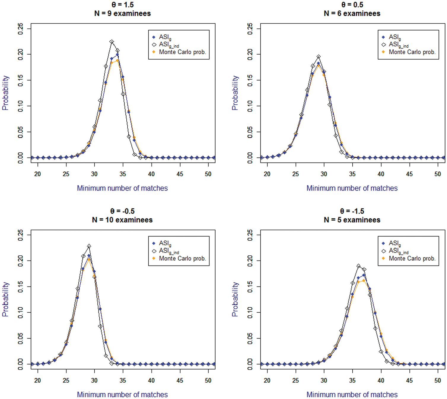
Figure 1 shows the distribution of the minimum number of matches calculated using ASI_g, ASI_{g_ind}, and the Monte Carlo method for a randomly selected cluster of size three across each simulated level of θ which had identified clusters. Although each of the distributions for each level of θ correspond fairly closely, one can see that the ASI_g and the Monte Carlo method correspond more closely to each other than to ASI_{g_ind}, indicating that the ASI_g appears to be a reasonable approach to approximating the probability each potential minimum number of matching responses (for clusters of size 3 in the given range of θ from −1.5 to 1.5), and that ASI_g’s approach to quantifying the dependence structure among the M_ij’s offers some benefit in comparison to ignoring the dependence. The deviation of ASI_{g_ind} from ASI_g appears larger at more extreme levels of θ (i.e., −1.5 and 1.5). It is worth noting that ASI_{g_ind} appears to underestimate the probabilities in the upper tail of the distribution, which is particularly problematic in a test security application.

Figure 1.

Distribution of the minimum number of matches $(M_{\min})$ for clusters of size three across varying θ levels: $AS I_{g}$ , $AS I_{g_ind}$ , and the Monte Carlo method.

While Figure 1 shows the distribution of the minimum number of matching responses for the smallest size clusters at each simulated ability level, Figure 2 shows the distributions of the largest size clusters (i.e., 9, 6, 10, and 5 for θ level 1.5, 0.5, −0.5, and −1.5, respectively). In comparison to the smaller-sized clusters, these distributions of M_min are narrower, and the deviation of ASI_{g_ind} from ASI_g is much larger. The difference between the probability of a potential minimum number of matching responses calculated by ASI_{g_ind} versus ASI_g is as high as 0.05 (for the probability of M_min = 36 matches in the cluster of 9 examinees at θ level 1.5). The same pattern that was observed for the clusters of size 3 emerges here where ASI_{g_ind} underestimates probabilities in the upper tail of the distribution.

Figure 2.

Distribution of the minimum number of matches $(M_{\min})$ for largest identified clusters across varying θ levels: $AS I_{g}$ , $AS I_{g_ind}$ , and the Monte Carlo method.

Rather than simply assessing the accuracy of probabilities estimated using ASI_g, we are interested in whether the use of ASI_g can be helpful in determining whether a cluster is spurious. As no collusion was simulated, all identified clusters are spurious. While the flagging criterion for a pair of examinees was 0.001, the mean p-value of ASI_g associated with the observed clusters was 0.006, with a minimum of 3.69 × 10⁻¹¹ and a maximum of 0.047. Thus, the p-values calculated using ASI_g were centered near the flagging criteria for pairs of examinees (i.e., 0.001).

When clusters of examinees mutually exhibit unusually similar response behavior, larger clusters will be associated with smaller p-values. However, in the case of spurious clusters like those shown in this simulation, there does not appear to be a relationship between cluster size and p-value. The correlation between cluster size and p-value for the 33 clusters of size three or greater identified in this simulation is −0.12, and the largest identified cluster (n_c = 10) has one of the larger p-values at 0.011. The distribution of p-values for the clusters is shown in Figure 3. Thus, it appears that the ASI_g can potentially aid in distinguishing between true collusion groups versus spurious clusters. If the same flagging criterion of 0.001 was used for clusters, 17 of the 33 clusters of three or more examinees would be flagged. While half of the clusters would still be flagged using this criterion, it is important to keep in mind that these clusters are not representative of the entire set of nonaberrant response behavior because they have already been identified using the WM method. Furthermore, it is not necessary to use the same flagging criterion for clusters as was used in the pairwise analysis.

Figure 3.

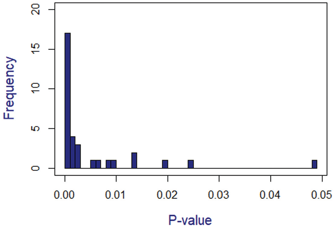
Distribution of p-values from the clusters identified in simulation.

A note on statistical power

Often methods introduced to detect test fraud include a simulation study with simulated collusion to assess the statistical power of the method. Without a meaningful comparison statistic, a simulation study assessing power of the ASI_g would be of somewhat limited utility because reported rates of statistical power are highly dependent on the ways in which collusion is simulated. A thorough simulation study of statistical power would enable us to observe predictable patterns that are well understood in the test security literature, ultimately showing that more egregious forms of collusion that are of more practical consequence (e.g., higher numbers of matching responses for intermediate ability examinees) have higher statistical power. In addition, a study of statistical power would be incomplete without a complementary study of Type-I error rate. Such a study for a group-level statistic such as ASI_g is less straightforward than for an individual-level statistic because it would involve evaluating all possible clusters of a given size in a simulated data set (or a large random sampling of clusters) rather than evaluating the response pattern of only each examinee. While a thorough investigation of power and Type-I error rates is beyond the scope of this article, Supplemental Appendix B includes a brief extension to the simulation study in this article with simulated collusion to help readers better understand the statistic, providing examples of detection rates of clearly defined clusters versus clusters with some spurious examinees.

Real Data

To illustrate how the ASI_g can be used to complement the WM methodology, an example is shown using real data from 1,992 examinees on a 60-item IT certification exam, where all items were published to a brain dump site on the internet. In addition to the complete item content, a key was also published to the site, but the key only showed correct responses for 24 of the 60 items. Item parameters were estimated using the Rasch model (which the testing program employs operationally) only using response data of the first 600 examinees chronologically, as the testing program had reason to believe that many response patterns after the first 600 were potentially contaminated by preknowledge of the exam content.

The WM method as described in the simulation section was applied to the data using a Bonferroni correction for multiple comparisons recommended by Wesolowsky (2000) when exploring all possible pairs of examinees, where the number of pairwise comparisons is used as the denominator for the Bonferroni adjustment. For α = 0.0001 at the test level, a flagging criterion of $0.0001 / ((1992 * 1991) / 2) = 5.0 * 10^{- 11}$ was used for flagging pairs of examinees. Using this criterion, four clusters of three or more examinees were detected and two additional pairs of examinees were detected. The clusters are described in Table 2 showing various properties and statistics associated with them, including the number of flagged examinees, the number of mutually flagged examinees (i.e., number of examinees who were all flagged with each other using the GBT in the cluster), the ranges of scores, and the p-value from the ASI_g, among others. The distribution of the number of matching responses for each cluster is also illustrated in Figure 4 showing the distribution of M_min calculated with ASI_g, ASI_{g_ind}, and the Monte Carlo method for each cluster.

Table 2.

Clusters From Information Technology Certification Data.

	Cluster
Descriptive statistic	1	2	3	4
No. of flagged examinees	36	16	7	3
No. of mutually flagged	20	11	0	0
Range of scores	37–40	38–40	22–26	36–38
Range of number matching	56–60	58–60	56–58	58–59
Range of expected number matching	37–38	38	36–37	37
$M_{\min}$	56	58	56	58
Percent of zero covariances	89.2%	76.5%	50.0%	0%
Average nonzero covariance	2.12	2.23	1.67	2.05
Average variance	13.19	13.12	13.58	13.48
ASI_g p-value	<1.06 × 10⁻³⁰⁰	2.58 × 10⁻¹⁸¹	3.63 × 10⁻⁷⁴	2.73 × 10⁻¹⁹

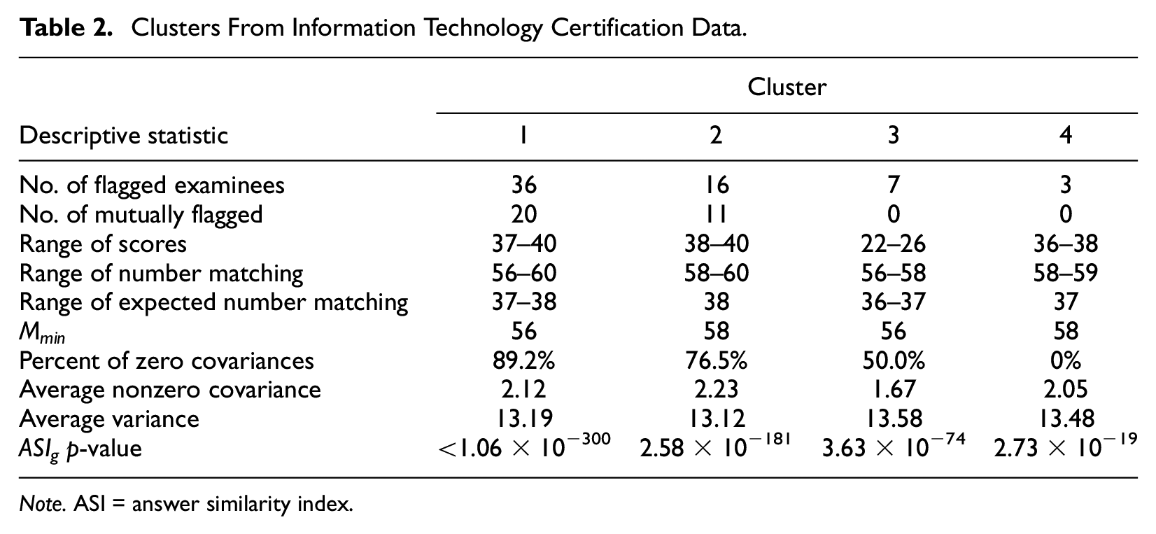
Note. ASI = answer similarity index.

The identified clusters ranged in size from three examinees (cluster 4) to 36 examinees (cluster 1). This wide range allows us to observe that larger clusters have a higher percentage of independent M_ij’s, indicated by the percentage of covariances in the covariance matrix which are equal to 0. For the largest cluster of 36 examinees, 89% of the covariances are equal to 0, whereas for the smallest cluster of 3 examinees, none of the covariances are equal to 0. Clusters 1 and 2 each have at least one pair of examinees with matching responses on all 60 items, whereas clusters 3 and 4 have a pairwise maximum number of matching responses of 58 and 59, respectively. Cluster 3 consisted of examinees whose responses corresponded closely to the key posted to the brain dump website, whereas examinees in the other clusters seemed to recognize that the posted key was incorrect and deviated from the posted key to achieve a higher score. The three clusters that deviated from the incorrect key appeared to be distinct as they did not exhibit very high overlap with each other; however, two of the clusters were more similar to each other than the third. The response patterns of the three examinees who were mutually flagged with the largest number of other examinees in each cluster were compared to each other, and exhibited pairwise numbers of matching responses of 44, 48, and 52 responses.

Average nonzero covariances are relatively small compared to average variances, which helps explain why the distributions of the number of matching responses calculated using ASI_{g_ind} are fairly similar to the corresponding distribution calculated using ASI_g and the Monte Carlo method. Each of the flagged clusters consisted of examinees who answered at least 20 items incorrectly. It is not surprising that the WM method did not produce clusters of examinees with higher scores due to the conservative pairwise flagging criterion.

In this example, the largest clusters showed much stronger evidence of group-level aberrance than the smaller clusters. P-values from ASI_g ranged from 2.73*10⁻¹⁹ for the smallest cluster to <1.06*10⁻³⁰⁰ for the largest cluster.¹ These p-values are extremely small in comparison to those calculated in the previously shown simulations using data with no simulated aberrance. The pattern of smaller p-values for larger clusters is expected to hold if the pairwise relationships among examinees in the clusters are similarly unusual. Similarly to the results shown in the simulation section, the distribution of the minimum number of matching responses is expected to be narrower for larger clusters of examinees. This pattern is illustrated in Figure 4 which shows the distribution of matching responses for each identified cluster calculated using ASI_g, ASI_{g_ind}, and the Monte Carlo method.

Figure 4.

Distribution of the minimum number of matches $(M_{\min})$ for identified clusters in information technology certification data: $AS I_{g}$ , $AS I_{g_ind}$ , and the Monte Carlo method.

Within each identified cluster, the range of scores is fairly small such that identified examinees have similar estimated abilities. For an additional real data example illustrating clusters of examinees with a larger range of scores, see Appendix D.

Discussion

The WM method proposes using the results from answer similarity analysis, which identifies unusually similar results among pairs of examinees, with cluster analysis to detect groups of examinees who may have colluded or had access to the same subset of exam content. While the WM method extends the use of answer similarity analysis from detecting unusually similar pairs of examinees to unusually similar clusters of examinees, the probabilistic statements enabled by the method still only apply to pairs of examinees.

The index introduced in this article, ASI_g, is used to estimate the probability that the minimum number of matching responses among a pair of examinees in the cluster is the observed minimum or greater, assuming examinees were working independently. While the method uses traditional answer similarity analysis, the statistical test relates to an entire cluster of examinees. Results showed that the ASI_g can be helpful in quantifying how unusual it is for large clusters of examinees to have similar response patterns, helping practitioners distinguish between spurious clusters of examinees and clusters of examinees who likely were involved in some sort of aberrant testing behavior. While this article presents the ASI_g as a probabilistic complement of the multistage WM approach, it could be used for clusters identified in other ways as well, such as reports from test proctors.

The method presented in this article describes one perspective of quantifying the dependence structure of groups of pairwise random variables (i.e., M_ij’s, the number of matching responses between pairs of examinees) to develop a general statistic for making inferences about the answer similarity of a group of examinees. However, several practical issues related to operational implementation of ASI_g have not been fully addressed in this article. First, the method may be infeasible for very large testing programs because the relationship between number of examinees and number of pairwise comparisons is exponential (affecting computational time for the pairwise similarity analysis), and the relationship between cluster size and the dimension of multivariate normal integration is also exponential (affecting computation time and feasibility of ASI_g calculations). For the data set analyzed in this procedure, computing all nearly two million pairwise comparisons of answer similarity took approximately 1 day using a standard laptop computer without using parallel processing. The $AS I_{g}$ calculation for the largest cluster of 36 examinees took about 15 minutes. Although computational methods for high dimensional multivariate normal integration is an active area of research (see, e.g., Azzimonti & Ginsbourger, 2018; Genton et al., 2018), the mvtnorm R package used for analysis in this article only handles problems with dimension 1,000 or less, accommodating clusters of 45 or fewer examinees.

Second, practitioners should assess whether all assumptions are reasonable for the particular application. Two main categories of assumptions should be checked: (a) the fit of the IRT model and (b) whether the multivariate normal distribution reasonably approximates the joint distribution of M_ij’s. The choice of the flagging criterion for the WM method will affect both categories of assumptions. The more liberal the flagging criterion, the more likely that examinees with more extreme scores (i.e., closer to perfect or closer to 0 scores) could be clustered together. Estimated ability levels for students with extreme scores often have large standard errors; thus, the probabilities resulting from the answer similarity analysis used in the clustering and as the basis for the ASI_g may not be accurate. In addition, as illustrated in Supplemental Appendix A, the normal approximation of the distribution of M_ij can be less accurate for pairs of examinees with more extreme ability estimates (i.e., either very high or very low ability). Thus, it is recommended that practitioners choose an appropriate flagging criterion for the WM method where they can be certain that assumptions of the ASI_g are reasonably met. Future research using both simulation and real data should thoroughly examine different conditions not explored in this article to help identify practical limitations of the method and establish guidelines for appropriate use.

Finally, this article has not addressed how practitioners should develop complete procedures and policies which could be used to take some sort of action based on the results of ASI_g. Semko and Hunt (2013) note that test sponsors should determine detection procedures and associated actions, which will be implemented fairly and in good faith, in advance of potential security breaches. In developing these policies and procedures, practitioners will need to determine how clusters will be formed and set flagging thresholds for the ASI_g, considering how the former will affect the latter. For example, if the WM method (using nearest-neighbor clustering) is used with a liberal flagging threshold to determine clusters, it is possible that an identified cluster could consist of two or more actual clusters that are weakly connected, leading the ASI_g probability to not reach the chosen threshold for flagging. If this example were to occur, practitioners could outline a method for disaggregating the cluster, adopt a more conservative flagging criterion for the WM method, use a different clustering method, or employ some combination of strategies. This hypothetical example illustrates that the method used to identify clusters is an important part in any set of detection policies and procedures which includes the use of ASI_g.

The current lack of published research comparing the various ways in which the WM methodology could be implemented is a limitation of the method presented in this article. In addition, research should be conducted on the ASI_g to show whether the normal approximation is appropriate for different conditions than those shown in the simulation, such as shorter tests. While additional research is needed on both the WM method and the ASI_g, as well as complete methodologies which could be used in practice for cluster selection and the use of ASI_g, any proposed methodology would need to be tailored to fit the needs of the individual program employing the methods, informed by the properties of their exams, the goals of the analysis, and what actions they would like to take based on the results.

Supplemental Material

sj-pdf-1-apm-10.1177_01466216211013109 – Supplemental material for Answer Similarity Analysis at the Group Level

Supplemental material, sj-pdf-1-apm-10.1177_01466216211013109 for Answer Similarity Analysis at the Group Level by Carol Eckerly in Applied Psychological Measurement

Footnotes

Declaration of Conflicting Interests

The author(s) declared no potential conflicts of interest with respect to the research, authorship, and/or publication of this article.

Funding

The author(s) received no financial support for the research, authorship, and/or publication of this article.

ORCID iD

Carol Eckerly

Supplemental Material

Supplemental material for this article is available online.

Notes

References

Andrews

D. F.

Gnanadesikan

Warner

J. L.

(1973). Methods for assessing multivariate normality. In Krishnaiah

P. R.

(Ed.), Proceedings of the International Symposium on Multivariate Analysis (Vol. 3, pp. 95–116). Academic Press.

Azzimonti

Ginsbourger

(2018). Estimating orthant probabilities of high dimensional Gaussian vectors with an application to set estimation. Journal of Computational and Graphical Statistics, 27(2), 255–267. https://doi.org/10.1080/10618600.2017.1360781

Belov

Wollack

J. A.

(2018). Detecting groups of examinees involved in test collusion [Paper presentation]. The annual meeting of the National Council on Measurement in Education, New York, NY, United States.

Blashfield

R. K.

Aldenderfer

M. S.

(1988), April. The methods and problems of cluster analysis. In Nesselroade

J. R.

Cattell

R. B.

(Eds.), Handbook of multivariate experimental psychology (pp. 447–474). Plenum Press.

Bock

R. D.

(1972). Estimating item parameters and latent ability when responses are scored in two or more nominal categories. Psychometrika, 37, 29–51.

Cizek

G. J.

Wollack

J. A.

(2017). Handbook of detecting cheating on tests. Routledge.

Genton

M. G.

Keyes

D. E.

Turkiyyah

(2018). Hierarchical decompositions for the computation of high-dimensional multivariate normal probabilities. Journal of Computational and Graphical Statistics, 27, 268–277. https://doi.org/10.1080/10618600.2017.1375936

Genz

(1992). Numerical computation of multivariate normal probabilities. Journal of Computational and Graphical Statistics, 1, 141–150.

Genz

Bretz

Miwa

Leisch

Scheipl

Bornkamp

Maechler

Hothorn

(2018). mvtnorm: Multivariate normal and t distributions (R package version 1.0-8). https://cran.r-project.org/web/packages/mvtnorm/

10.

Gocer Sahin

Wollack

J. A.

(2018), October. Evaluation of different clustering approaches in detection of test collusion [Paper presentation]. The conference on Test Security, Park City, UT, United States.

11.

Haberman

S. J.

Lee

Y.-H.

(2017). A statistical procedure for testing unusually frequent exactly matching responses and nearly matching responses (Research Report No. RR-17-23). Educational Testing Service. https://doi.org/10.1002/ets2.12150

12.

Johnson

R. A.

Wichern

D. W.

(1998). Applied multivariate statistical analysis (4th ed.). Prentice Hall.

13.

Lathrop

Q. N.

(2015). cacIRT: Classification accuracy and consistency under item response theory (R Package Version 1.4). https://CRAN.R-project.org/package=cacIRT

14.

Lehmann

E. L.

(1999). Elements of large-sample theory. Springer.

15.

Lord

F. M.

Wingersky

M. S.

(1984). Comparison of IRT true-score and equipercentile observed-score “equatings.” Applied Psychological Measurement, 8, 452–461.

16.

Maynes

D. D.

(2014). Detection of non-independent test taking by similarity analysis. In Kingston

N. M.

Clark

A. K.

(Eds.), Test fraud: Statistical detection and methodology (pp. 53–82). Routledge.

17.

Maynes

D. D.

(2017). Detecting potential collusion among individual examinees using similarity analysis. In Cizek

G. J.

Wollack

J. A.

(Eds.), Handbook of quantitative methods for detecting cheating on tests (pp. 47–69). Routledge.

18.

Rasch

(1980). Probabilistic models for some intelligence and attainment tests. University of Chicago Press. (Original work published 1960)

19.

R Core Team. (2018). R: A language and environment for statistical computing. R Foundation for Statistical Computing. https://www.R-project.org/

20.

Semko

J. A.

Hunt

(2013). Legal matters in test security. In Wollack

J. A.

Fremer

J. J.

(Eds.), Handbook of test security (pp. 237–258). Routledge.

21.

van der Linden

W. J.

Sotaridona

(2006). Detecting answer copying when the regular response process follows a known response model. Journal of Educational and Behavioral Statistics, 31(3), 283–304. https://doi.org/10.3102/10769986031003283

22.

Wesolowsky

G. O.

(2000). Detecting excessive similarity in answers on multiple choice exams. Journal of Applied Statistics, 27(7), 909–921.

23.

Wollack

J. A.

Maynes

D. M.

(2017). Detection of test collusion using cluster analysis. In Cizek

G. J.

Wollack

J. A.

(Eds.), Handbook of quantitative methods for detecting cheating on tests (pp. 124–150). Routledge.

24.

Yates

(1934). Contingency table involving small numbers and the

χ^{2}

test. Journal of the Royal Statistical Society, 1(2), 217–235.

25.

Zopluoglu

(2017). Similarity, answer copying, and aberrance: Understanding the status quo. In Cizek

G. J.

Wollack

J. A.

(Eds.), Handbook of quantitative methods for detecting cheating on tests (pp. 25–46). Routledge.

26.

Zopluoglu

(2018). CopyDetect: Computing response similarity indices for multiple-choice tests (R Package Version 1.3). https://cran.r-project.org/web/packages/CopyDetect/index.html

Supplementary Material

Please find the following supplemental material available below.

For Open Access articles published under a Creative Commons License, all supplemental material carries the same license as the article it is associated with.

For non-Open Access articles published, all supplemental material carries a non-exclusive license, and permission requests for re-use of supplemental material or any part of supplemental material shall be sent directly to the copyright owner as specified in the copyright notice associated with the article.

0.00 MB

0.32 MB