Differential Volume and Price Reactions to Loss Announcements and the Association With Loss Reversals

Abstract

We examine differential volume–price reactions to loss announcements and their association with loss reversals. Our findings show that differential volume–price reactions are dissimilar between firms reporting profits and losses. In addition, the differential volume–price reactions surrounding loss announcements are useful in predicting loss reversals. When jointly considered, volume and price reactions provide unique information about future profitability for firms currently reporting losses. Overall, our results are consistent with losses generating more investor disagreements and more trading volume and show that a measure based on differential volume–price reactions to loss announcements is informative with regard to predicting subsequent loss reversals.

Keywords

abnormal trading volume earnings announcements differential volume and price losses loss reversals trading volume

Introduction

The prevalence of losses has increased significantly in the United States in the last several years (Collins, Pincus, & Xie, 1999; Hayn, 1995; Joos & Plesko, 2005; Klein & Marquardt, 2006). Prior research shows that the valuation of firms announcing losses and their returns–earnings relation is different than for profitable firms (Darrough & Ye, 2007; Franzen & Radhakrishnan, 2009; Hayn, 1995). Loss announcements generally lead to more investor disagreement about a firm’s future prospects and its potential return to profitability. Predicting loss reversals has thus been a topic of considerable interest in the accounting literature (e.g., Jiang & Stark, 2011; Joos & Plesko, 2005; Li, 2011). We add to this body of literature through our examination of a measure that incorporates the information from both volume and price reactions to earnings announcements into one metric. To our knowledge, we are the first to jointly consider the volume and price reactions to earnings loss announcements in demonstrating the unique information a joint consideration offers in predicting loss reversals.

The theoretical relationship between volume and price is complex and depends not just on the dispersion of beliefs but also on the specific nature of belief revisions (Milgrom & Stokey, 1982; Shalen, 1993). For this reason, theory suggests that studying both volume and price reactions can provide a deeper understanding of the information environment surrounding an earnings report than studying either in isolation.

There are a number of prior empirical research papers examining volume reactions in addition to price reactions (Atiase & Bamber 1994; Bamber, 1986; Bamber & Cheon, 1995; Beaver, 1968; Kiger, 1972; Morse, 1981). Beaver (1968) suggests that relative to price reactions, volume reactions have the potential to provide better insights on the usefulness of public disclosures. Bamber and Cheon (1995) examine differential volume and price reactions to earnings announcements and conclude their empirical analysis stating that the “observed relation between trading volume and price reactions is closer to independence than a strong positive relation” (p. 440).

Trading volume and abnormal trading volume around earnings announcements have increased significantly in recent periods (Ahmed, Schneible, & Stevens, 2003; Bailey, Li, Mao, & Zhong, 2003; Barron, Byard, & Yu, 2010; Barron, Schneible, & Stevens, 2009; Landsman & Maydew, 2002). While price movements reflect changes in the market’s average beliefs, trading volume is the sum of all individual investors’ trades (Kim & Verrecchia, 1991b). Loss announcements have the potential to increase uncertainty, and hence are more likely to generate greater investor disagreements leading to greater volume reactions. In the context of loss announcements, volume reactions in conjunction with observed price reactions may also contain information relating to subsequent earnings and return to profitability for the firm. Our study of differential volume–price reactions for loss firms contributes to a better understanding of investor perceptions regarding loss announcements. We use differential volume–price reactions as modeled by Bamber and Cheon (1995) to isolate the unique information about disaggregated beliefs afforded by joint examination of trading volume and price reactions. Specifically, the measure that we use captures the differences in magnitude between volume and price reactions to a loss announcement.¹ We examine whether using such a measure helps in better predicting reversals of losses in future periods.

We focus on abnormal trading volume and abnormal returns surrounding earnings announcements. Abnormal trading volume, which is trading volume adjusted for normal liquidity trading, assesses the degree to which the market agrees on the consensus price. Abnormal return assesses the degree to which the consensus price is adjusted in response to the new information. We incorporate the relative strength of these two reactions in our operational measure RANKDIFF, computed as the decile rank of abnormal trading volume less the decile rank of abnormal return. Our metric RANKDIFF measures the earnings announcement effect on the magnitude of belief disaggregation relative to the magnitude of belief revision. Where the decile rank of abnormal volume is larger (smaller) than the decile rank of abnormal return, RANKDIFF is positive (negative). Therefore, a positive RANKDIFF would suggest that the effect of the newly arrived information created disaggregation in beliefs more than it revised the consensus belief. We posit and find that RANKDIFF is different between profit and loss firms and that, for loss firms, this metric contains information that is valuable in predicting future profitability.

Our empirical analyses extend over 1990-2013 and use a sample of 54,792 firm-year observations, 16,272 of which are loss announcements. In examining differential volume and price reactions, we find that a significant number of loss earnings announcements generate either large volume–small price or small volume–large price reactions.

Joos and Plesko (2005) use accounting and other variables to predict loss reversals. Our results show that using differential volume–price reactions in addition to accounting and other variables improves the predictive ability of their models. Our results show that RANKDIFF, our operational measure that captures the observed differential volume and price reactions, has predictive power relating to subsequent loss reversals and that using RANKDIFF is superior to using individual volume and price reaction measures alone.

Our results also suggest that large volume–small price reactions are associated with subsequent loss reversals. Large volume reactions suggest that investors’ belief changes have been in different directions with many traders revising upward (wishing to buy) while an equal number have revised downward and are willing to sell. The net effect on the price change may therefore be small though a large number of transactions will take place. Thus, our results suggest that when volume is high relative to price changes, the probability that losses are likely to reverse increases. In addition, our results show that the probability of loss reversal decreases when the loss event is associated with low volume–large price reactions. These results have potential value to policy makers and regulators concerned with the impact of accounting disclosures, and to those who view market reactions as a measure of the disclosure’s usefulness to investors.

Overall, our article contributes to the literature relating to differential volume–price reactions to financial disclosures, particularly loss announcements. In addition, our article contributes to the literature examining losses and predicting loss reversals.

The remainder of the article is organized as follows. The “Conceptual Underpinnings” section develops the study’s conceptual underpinnings. The “Research Method and Results” section discusses research methodology and results. A brief summary and concluding comments are provided in the “Discussion and Conclusion” section.

Conceptual Underpinnings

We first discuss research examining volume reactions to earnings announcements. We then draw from studies that examine losses and loss reversals to develop our motivations for inclusion of differential volume–price metrics to examine loss reversals.

Earnings and Trading Volume

Both volume and price reactions to disclosures arise from belief revisions of investors. While price reactions reflect investors’ average belief revision in the aggregate (Beaver, 1968; Kim & Verrecchia 1991a, 1991b), trading volume reactions reflect the diversity in investors’ prior beliefs and differential belief revisions (Bamber, 1986, 1987; Barron, 1995; Karpoff, 1986; Kim & Verrecchia, 1991a, 1991b).² Theoretical literature relating to volume (Harris & Raviv, 1993; Kandel & Pearson, 1995; Milgrom & Stokey, 1982; Shalen, 1993) predicts that increased divergence of opinion among investors spurs greater trading volume. Banerjee and Kremer (2010) allow for investors having heterogeneous prior beliefs and heterogeneous belief revisions. They show that under these settings, trading volume reflects revisions to the levels of disagreements. Empirically, Atiase and Bamber (1994) examine annual earnings announcements and provide evidence that the level of predisclosure information asymmetry influences the magnitude of the trading volume reaction. Barron, Harris, and Stanford (2005) show that abnormal trading volume around earnings announcements increases as the proxy for information asymmetry increases.

The results of these studies are consistent with the theoretical predictions that investor disagreements and consequent divergence of beliefs lead to larger volume reactions. The results are also consistent with the interpretation that trading volume reactions to earnings announcements contain information.

Loss Announcements and Loss Reversals

To our knowledge, no prior study has examined trading volume reactions to loss announcements. However, studies have examined price reactions to loss announcements and show differences in the magnitude of price reactions to profit and loss announcements (e.g., Collins et al., 1999; Hayn, 1995). Hayn (1995) shows a strong positive association between earnings and returns for profit announcements, but weak or no correlation with contemporaneous price movements for loss announcements. Other studies (e.g., Collins et al., 1999; Jan & Ou, 1995) demonstrate that the price–earnings relation is not only different for firms reporting profits and losses but also actually negative for firms reporting losses.

Studies have also examined loss reversals. Joos and Plesko (2005) and Jiang and Stark (2011) develop loss reversal models using accounting information. Li (2011) extends Joos and Plesko’s findings to develop a model that forecasts future earnings of loss firms. Dhaliwal, Kaplan, Laux, and Weisbrod (2012) examine the information content of tax expense for firms reporting losses. Almost all these studies rely on price and accounting information–based metrics such as cash flow from operations, accruals, and return on assets in examining these issues. None of these studies use any volume-based measure or measures that combine both volume and price reactions in examining loss reversals.

Trading Volume, Differential Volume–Price Reactions, and Loss Reversals

Trading volume is used as a measure of investor reaction in numerous prior empirical studies.³Beaver (1968) identifies trading volume as having the potential to provide unique insights relating to the usefulness of financial disclosures. Bamber, Barron, and Stevens (2011) suggest that trading volume may provide the clearest evidence that a financial disclosure influences investors’ expectations and investment choices. In addition, they argue that trading volume has the potential to provide insights regarding investor disagreements consequent to financial disclosures. Cochrane (2007) suggests that asset pricing could benefit tremendously from models that would enable interpreting empirically observed levels and patterns in trading volume. Overall, the volume literature provides substantial evidence that trading volume has information content and is useful in evaluating the impact that financial disclosures have on investors.

While most studies examine either volume or price reactions to financial disclosures separately, Bamber and Cheon (1995) examine differential volume–price reactions to earnings announcements. Using quarterly earnings announcements for the 1986-1989 period, they document that a significant percentage of earnings announcements (approximately 20%-24%) generate either very large (small) trading or very small (large) price change. They also show that large volume–small price reactions are associated with divergent analyst forecasts, greater analyst following, larger unexpected earnings, and stock price increases (Bamber & Cheon, 1995).⁴

Differential reaction between volume and price as modeled by Bamber and Cheon (1995) isolates the unique information afforded by trading volume. Volume and price reactions partially reflect duplicate information. Differential volume–price reactions capture the unique portion of trading volume not reflected in price movement. Prices will respond to the loss event, but the larger trading volume relative to a lower price change reflects the heterogeneity of beliefs regarding the probability of a loss reversal. In summary, we expect that volume reactions and a measure that captures both volume and price reactions are likely to reflect information that is useful in the prediction of loss reversals.

When the consensus is that loss reversal is unlikely, the price will drop significantly, perhaps resulting in significant levels of trade. In contrast, when there is disagreement on whether a loss reversal is likely, the price reaction will be low relative to that of volume. The differential reaction measure that we use (RANKDIFF) summarizes this level of disaggregation of beliefs or disagreement.⁵ We believe that this aggregate measure of disagreement at the time of loss announcement will add to our understanding of loss reversals. To the extent that loss events generate heterogeneous beliefs, the uncertainty of loss reversals is expected to incrementally increase heterogeneity and be captured in differential volume–price reactions. Specifically, we expect that greater investor disagreements as captured by the differential volume–price reactions are likely to be positively associated with loss reversals.

Research Method and Results

Sample

We obtain 322,369 annual earnings announcements from the Compustat database for the period 1990-2012.⁶ A total of 140,037 firm-years were dropped due to insufficient price or volume information. Firms with less than US$5 million in total assets (3,534 firm-years) and firm-years with missing income data or balance sheet data (124,006 firm-years) were also dropped. This results in a sample of 54,792 firm-years for our examination of differential reactions relative to firm profitability.⁷ Table 1 presents the details of our sample selection.

Table 1.

Sample Selection.

	Firm-years
Firm-years from Compustat, 1990-2012	322,369
Less: Insufficient volume or price information	140,037
Less: Missing financial data for reversal models	124,006
Less: Firms with less than US$5 million in total assets	3,534
Firm-year observations used in initial contingency table	54,792
Total firm-years	54,792
Profit firm-years	38,520
Loss firm-years
Total loss firm-years in sample	16,272
Current period losses not reporting 1 year ahead	1,746
Current period losses included in reversal estimations	14,526
Current period losses reversing 1 year ahead	4,119
Current period losses also reporting a loss 1 year ahead	10,407
	14,526

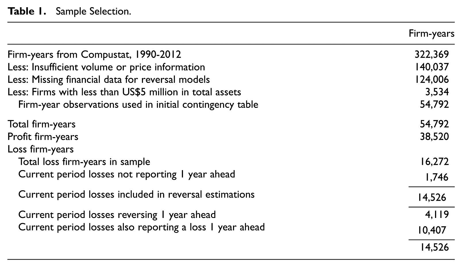
Table 1 also provides description of frequency and reversal of losses in our sample. Following Hayn (1995), we use income (loss) from continuing operations, before extraordinary items, discontinued operations, and the cumulative effect of accounting changes to define our earnings variable. Based on this measure, of the total 54,792 firm-years, 38,520 (70.30%) represent profit years, whereas the remaining 16,272 (29.70%) represent loss firm-years. A total of 1,746 loss firms are not included in the data set 1 year ahead and are therefore not included in our analysis of loss reversal. Of the loss firm-years included in our analysis of loss reversals (14,526), a total of 4,119 (28.36%) reverse in the immediate next period and 1,861 (12.81%) reverse in the second period following the loss. A total of 6,904 (47.53%) loss firm-years continue to have losses for 2 or more years following the initial loss.⁸

Table 2 shows distribution of losses over the years in our sample. The incidence of losses ranges from a low of 16.85% in 1990 to a high of 44.08% in 2001. As documented in other studies (e.g., Hayn, 1995; Li, 2011), loss announcements are over a fifth (20%) of observations after the 1990s.⁹

Table 2.

Sample Distribution Over Time.

Fiscal year	Profit firm-years	Loss firm-years	Total firm-years	% loss
1990	1,095	222	1,317	17
1991	1,280	386	1,666	23
1992	1,437	426	1,863	23
1993	1,604	548	2,152	25
1994	1,706	414	2,120	20
1995	1,821	598	2,419	25
1996	1,948	711	2,659	27
1997	1,953	818	2,771	30
1998	1,808	878	2,686	33
1999	1,856	1,098	2,954	37
2000	1,580	1,089	2,669	41
2001	1,342	1,058	2,400	44
2002	1,432	834	2,266	37
2003	1,630	767	2,397	32
2004	1,786	647	2,433	27
2005	1,773	628	2,401	26
2006	1,765	597	2,362	25
2007	1,656	615	2,271	27
2008	1,331	717	2,048	35
2009	1,437	762	2,199	35
2010	1,589	547	2,136	26
2011	1,624	579	2,203	26
2012	1,526	609	2,135	29
2013	1,541	724	2,265	32
Total	38,520	16,272	54,792	30

Note. The table provides the observations by year for our full sample, for firm-years where the earnings announcement indicated positive earnings (profit firm-years), and for firm-years where the earnings announcement indicated negative earnings (loss firm-years), respectively.

Trading Volume Measures

Several measures of volume have been used in prior studies. Recent research (e.g., Garfinkel, 2009; Garfinkel & Sokobin, 2006) suggests use of adjusted trading volume (i.e., abnormal volume). Garfinkel (2009) observes that abnormal volume may be the best indicator of divergent investor beliefs. Bamber et al. (2011) favor an examination of adjusted volume measures to mitigate potential problems such as measurement error and correlated omitted variables. We use two measures of adjusted or abnormal trading volume, denoted AVMM and AVDD. We estimate normal trading volume using a non-announcement period beginning on the 50th trading day prior to the announcement date and ending the 11th day prior to the announcement date, consistent with Bamber and Cheon (1995).

For our first measure of abnormal trading volume, AVMM, we regress firm trading volume on market volume and the firm’s market value of equity during the nonannouncement period (Bamber, Barron, & Stober, 1999). The dependent variable is daily trading volume divided by the number of shares outstanding. Market volume is measured as market-wide trading volume divided by the market-wide shares outstanding. The firm’s market value of equity is computed as the closing share price on the day prior to the announcement. We predict daily trading volume for the announcement period using the parameter estimates obtained from the nonannouncement period regression.¹⁰ We define AVMM as the difference between the forecasted and actual trading volume cumulated over the announcement window.

Our second measure of abnormal trading volume (AVDD) is calculated using a difference-in-differences approach. We define a firm’s (market’s) unadjusted abnormal trading volume as the percentage of firm (market) shares trading during the firm’s announcement period less the average percentage of firm (market) shares trading during the firm’s nonannouncement period. AVDD is the firm’s unadjusted abnormal trading volume less the market-wide fluctuations in trading volume.¹¹

Table 3 presents descriptive statistics for the volume measures employed in our analyses.¹² Panel A of Table 3 shows descriptive statistics for the full sample, whereas Panels B and C present descriptive statistics separately for the profit and loss firm-years, respectively. The mean and median values for both AVMM and AVDD are lower for loss firm-years compared with profit firm-years. The mean value for AVMM for loss (profit) firm-years is 0.0100 (0.0143), and the median value is 0.0021 (0.0047). The mean value of AVDD for loss (profit) firms is 0.0133 (0.0160), and the median value is 0.0025 (0.0048). Tests for differences in means between loss and profit firm-years for AVMM and AVDD are significant at p < .01.¹³

Table 3.

Descriptive Statistics for Return and Volume Metrics.

Panel A: Full Sample.
Variable	M	25th percentile	Median	75th percentile	SD	Observations
AVMM	0.0130	(0.0019)	0.0039	0.0186	0.0382	54,792
AVDD	0.0152	(0.0020)	0.0041	0.0189	0.0365	54,792
CAR	0.0613	0.0173	0.0406	0.0819	0.0644	54,792
Panel B: Profit Firm-Years.
Variable	M	25th percentile	Median	75th percentile	SD	Observations
AVMM	0.0143	(0.0011)	0.0047	0.0195	0.0363	38,520
AVDD	0.0160	(0.0013)	0.0048	0.0196	0.0352	38,520
CAR	0.0543	0.0155	0.0363	0.0722	0.0571	38,520
Panel C: Loss Firm-Years.
Variable	M	25th percentile	Median	75th percentile	SD	Observations
AVMM	0.0100	(0.0046)	0.0021	0.0163	0.0424	16,272
AVDD	0.0133	(0.0043)	0.0025	0.0166	0.0395	16,272
CAR	0.0781	0.0232	0.0539	0.1066	0.0764	16,272

Note. The table provides descriptive statistics for volume and return variables used in the analyses. Panels A, B, and C provide the statistics for the full sample, for firm-years where the earnings announcement indicated positive earnings (profit firm-years), and for firm-years where the earnings announcement indicated negative earnings (loss firm-years), respectively. Descriptions for the variables are provided in the appendix. Results for differences between mean values (t test) of variables for profit and loss firm-years show that all variables are significantly different at p < .01.

Differential Volume and Price Reactions Around Loss Announcements

Empirical tests based on our conceptual framework call for developing differential volume–price measures. Our measures of volume are AVMM and AVDD. However, to develop measures of differential volume–price, we calculate cumulative abnormal returns for a 3-day window (−1, 0, and +1, where 0 is the earnings announcement day) around earnings announcements. We then adopt methodology similar to Bamber and Cheon (1995) to develop our differential price–volume measure. Following the contingency table format employed by Bamber and Cheon, we separately decile rank the abnormal trading volume (i.e., AVMM)¹⁴ and return (i.e., CAR) variables in the earnings announcement period. We label similar reactions to those where the absolute value of the difference between the volume and return decile rankings is less than 3. Observations where the decile ranking for volume (price) exceeds that of price (volume) by 5 or more are classified as large volume–small price (small volume–large price). The remaining observations (those observations where the difference between volume and price deciles is between 2 and 5) are classified as indeterminate. Table 4 presents the contingency table results for volume–price decile classifications.

Table 4.

Contingency Tables of Volume Reaction Deciles by Price Reaction Deciles.

Panel A: Bamber and Cheon (1995).
	Similar reactions^a	Indeterminate reactions^a	Large volume and small price^a	Small volume and large price^a
1. Expected frequency under the null hypothesis of independence (%)
	44.00	26.00	15.00	15.00
2. Results (n = 8,180)
	52.26%	25.21%	11.22%	11.31%
	(50.60%-53.92%)	[23.77%, 26.65%]	[10.17%, 12.27%]	[10.26%, 12.36%]
Panel B: Current Results.
	Similar reactions^a	Indeterminate reactions^a	Large volume and small price^a	Small volume and large price^a
3. Full sample of annual announcements, 1990-2013 (n = 54,792)
	56.56%	24.40%	9.10%	9.94%
	[54.64%, 58.48%]	[22.9%, 25.9%]	[7.51%, 10.7%]	[8.37%, 11.51%]
4. Loss firm-years (n = 16,272)
	51.00%	23.69%	6.88%	18.44%
	[49.66%, 52.33%]	[22.52%, 24.87%]	[5.48%, 8.27%]	[17.24%, 19.64%]
5. Profit firm-years (n = 38,520)
	58.91%	24.70%	10.04%	6.35%
	[56.61%, 61.21%]	[22.89%, 26.51%]	[8.17%, 11.91%]	[4.36%, 8.34%]
Conditioned on prior profitability
6. Loss firms with previous period loss (n = 11,203)
	50.08%	23.64%	6.42%	19.87%
	[48.75%, 51.4%]	[22.43%, 24.85%]	[4.97%, 7.86%]	[18.59%, 21.15%]
7. Loss firms with previous period profit (n = 5,069)
	53.03%	23.81%	7.89%	15.27%
	[51.57%, 54.49%]	[22.62%, 25.01%]	[6.53%, 9.25%]	[14.09%, 16.45%]
Conditioned on future profitability
8. Loss firms with loss in next period (n = 10,407)
	49.88%	23.83%	6.16%	20.13%
	[48.55%, 51.21%]	[22.61%, 25.05%]	[4.69%, 7.63%]	[18.83%, 21.43%]
9. Loss firms with profit in next period (n = 4,119)
	54.21%	24.33%	8.33%	13.13%
	[52.62%, 55.8%]	[23.06%, 25.59%]	[6.92%, 9.73%]	[11.87%, 14.4%]

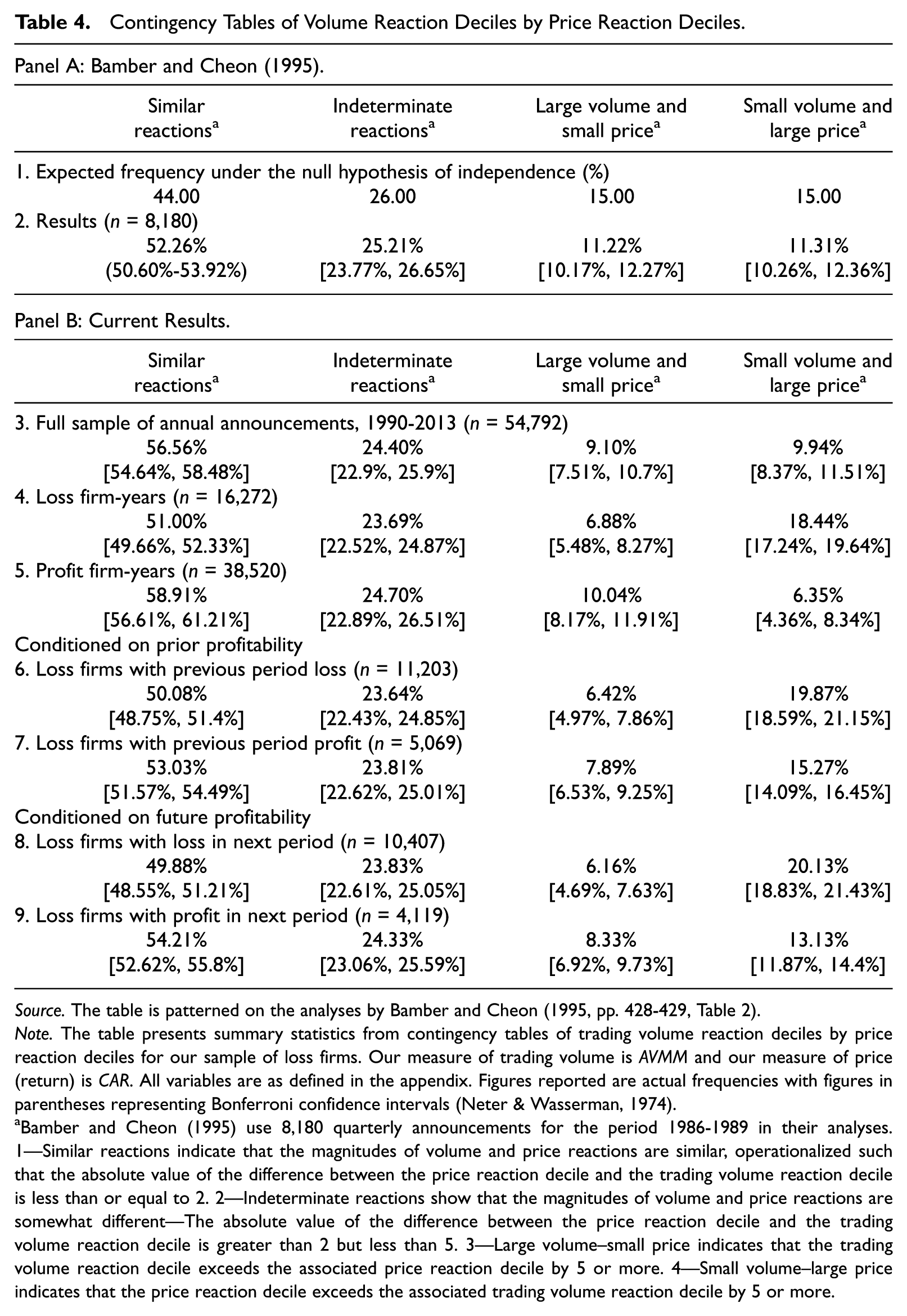
Source. The table is patterned on the analyses by Bamber and Cheon (1995, pp. 428-429, Table 2).

Note. The table presents summary statistics from contingency tables of trading volume reaction deciles by price reaction deciles for our sample of loss firms. Our measure of trading volume is AVMM and our measure of price (return) is CAR. All variables are as defined in the appendix. Figures reported are actual frequencies with figures in parentheses representing Bonferroni confidence intervals (Neter & Wasserman, 1974).

Bamber and Cheon (1995) use 8,180 quarterly announcements for the period 1986-1989 in their analyses. 1—Similar reactions indicate that the magnitudes of volume and price reactions are similar, operationalized such that the absolute value of the difference between the price reaction decile and the trading volume reaction decile is less than or equal to 2. 2—Indeterminate reactions show that the magnitudes of volume and price reactions are somewhat different—The absolute value of the difference between the price reaction decile and the trading volume reaction decile is greater than 2 but less than 5. 3—Large volume–small price indicates that the trading volume reaction decile exceeds the associated price reaction decile by 5 or more. 4—Small volume–large price indicates that the price reaction decile exceeds the associated trading volume reaction decile by 5 or more.

Table 4 shows the expected percentage of reactions in each of the four categories (similar, indeterminate, large volume–small price, and small volume–large price reactions) under the null hypotheses of independence of volume and price reactions followed by the actual observed percentages. Also reported are the two-tailed 99% Bonferroni confidence intervals (Neter & Wasserman, 1974; Neter, Wasserman, & Kutner, 1983).¹⁵ For comparison purposes, we provide the Bamber and Cheon (1995) results in Panel A. In Panel B of Table 4, we report results for our full sample and also separately for loss and profit announcement years. Our full sample results appear similar to those of Bamber and Cheon. For example, 56.56% of our observations are classified in the similar category, where 52.26% of the observations analyzed by Bamber and Cheon fall into the same category.¹⁶ Figures for the other three categories are also similar to those found in Bamber and Cheon. Our results for the full sample do not support the conclusion of independence between volume and price reactions.

The volume–price reactions for loss and profit firm-years are markedly dissimilar. Only 51.00% of the loss observations are classified as similar compared with 58.91% for profit firm-years. Furthermore, the observed percentage for loss firm-years (51.00%) is well outside of the 99% confidence interval for profit firm-years (from 56.61% to 61.21%). The most notable difference between loss and profit firm-years occurs in the large volume–small price and small volume–large price classifications. These two classifications show that the relative magnitude of volume and price reactions is very different for 25.32% (6.88% + 18.44%) of loss year announcements, compared with 16.39% (10.04% + 6.35%) of profit year announcements.¹⁷

Classifications for loss firm-years based on prior profitability and future profitability also differ both in the large volume–small price and in the small volume–large price categories. Overall, these results in Table 4 show that differential volume–price reactions are different for loss firm-year and profit firm-year announcements.¹⁸ Our results further suggest that differential volume–price reactions differ for loss firms dependent upon future profitability.

Predicting Loss Reversals

We suggest that differential volume and price reactions to loss announcements are reflective of a belief revision process. The literature regarding loss reversals (e.g., Jiang & Stark, 2011; Joos & Plesko, 2005; Li, 2011) examines the predictive power of accounting measures corresponding to the report of earnings. Our interest is in the predictive nature of the belief revision process surrounding an earnings loss announcement. Specifically, we are interested in evaluating the predictive nature of the belief revision pattern rather than the financial numbers upon which the revisions are made. We now examine if the belief revision process, as measured by differential volume–price reactions, contains information about future loss reversals.

Differential volume–price reactions metric as a predictor

We examine if a measure that captures the relative magnitude of the differential volume–price reactions, as presented in Table 4, has predictive ability. We define the variable RANKDIFF as the decile ranking of volume (RANK_VOL) less the decile ranking of price (RANK_RET), where the decile rankings of volume and price are as described before. Higher values of RANKDIFF indicate larger volume and small price reactions. Thus, a positive coefficient on RANKDIFF in a loss-reversal prediction model will mean that larger volume–small price reactions are indicators of loss reversals. RANKDIFF captures information contained in both volume and price reactions. It summarizes the level of disaggregation of beliefs or disagreements surrounding earnings announcements relative to the change in the consensus of beliefs (return). As discussed previously, RANKDIFF is also likely to reflect significant information regarding beliefs of market participants that is useful in the prediction of loss reversals.

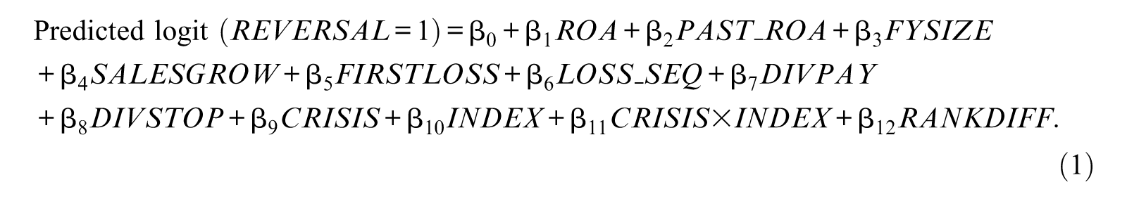
We estimate logit regressions where the dependent variable is coded as 1 if the loss for the firm reverses in the next year, and 0 otherwise. Our regression models include all variables included in the original Joos and Plesko (2005) model specifications plus our variable of interest RANKDIFF. In addition, we include three economic control variables. CRISIS is an indicator variable that takes on a value of 1 if the observation pertained to years 2008-2010, and 0 otherwise. This variable is included to control for the financial crash of 2008, whose effects continued and lingered in substantive fashion for 2009 and 2010 as well. INDEX is a scale variable that we use to control for economic effects and is the “Leading Index for the United States” published by the Federal Reserve Bank of Philadelphia. The Leading Index utilizes multiple economic inputs to provide a composite index capturing economic trends and expectations. In addition to these two variables, we include the interactive term CRISIS×INDEX in our analyses. The models that we estimate are as follows:

Model I (based on Joos & Plesko’s, 2005, Specification 1):

\begin{matrix} Predicted logit (REVERSAL = 1) = β_{0} + β_{1} ROA + β_{2} PAST_ROA + β_{3} FYSIZE \\ + β_{4} SALESGROW + β_{5} FIRSTLOSS + β_{6} LOSS_SEQ + β_{7} DIVPAY \\ + β_{8} DIVSTOP + β_{9} CRISIS + β_{10} INDEX + β_{11} CRISIS \times INDEX + β_{12} RANKDIFF . \end{matrix}

Model II (based on Joos & Plesko’s, 2005, Specification 2):

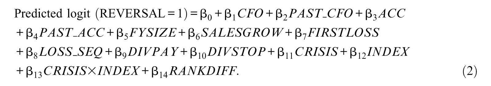
\begin{array}{l} Predicted logit (REVERSAL = 1) = β_{0} + β_{1} C F O + β_{2} PAST_CFO + β_{3} ACC \\ + β_{4} PAST_ACC + β_{5} FYSIZE + β_{6} SALESGROW + β_{7} FIRSTLOSS \\ + β_{8} LOSS_SEQ + β_{9} DIVPAY + β_{10} DIVSTOP + β_{11} CRISIS + β_{12} INDEX \\ + β_{13} CRISIS \times INDEX + β_{14} RANKDIFF . \end{array}

All variables in these models are as defined in the appendix. The operational measures for these variables (other than for CRISIS, INDEX, CRISIS×INDEX, and RANKDIFF) are identical to those used in Joos and Plesko (2005). Table 5 presents descriptive statistics for all the variables used in our regression estimations. Panel A of Table 5 shows descriptive statistics for the full sample, whereas Panels B and C present descriptive statistics separately for the profit and loss firm-years, respectively. Tests for differences in mean values for the independent variables used in our regression are significantly different at p < .01, across profit and loss firm-years.

Table 5.

Descriptive Statistics.

Panel A: Full Sample.
Variable	M	25th percentile	Median	75th percentile	SD	Observations
Differential volume and return metric
RANKDIFF	0.0000	(2.0000)	0.0000	2.0000	3.3807	54,792
Joos and Plesko reversal variables
ACC	(0.0144)	(0.0030)	(0.0001)	0.0011	0.2486	54,792
CFO	0.0466	0.0186	0.0834	0.1428	0.2170	54,792
DIVPAY	0.4502	0.0000	0.0000	1.0000	0.4975	54,792
DIVSTOP	0.0393	0.0000	0.0000	0.0000	0.1944	54,792
FIRSTLOSS	0.0567	0.0000	0.0000	0.0000	0.2312	54,792
FYSIZE	6.2135	4.7496	6.0697	7.5436	2.0008	54,792
LOSS_SEQ	1.0711	0.0000	0.0000	1.0000	1.9428	54,792
ROA	(0.0212)	(0.0210)	0.0399	0.0882	0.2713	54,792
SALESGROW	0.2368	(0.0014)	0.0975	0.2672	0.6308	54,792
PAST_ACC	(0.0162)	(0.0004)	0.0000	0.0003	0.2626	54,792
PAST_CFO	0.0289	0.0000	0.0736	0.1271	0.2242	54,792
PAST_ROA	(0.0411)	(0.0155)	0.0376	0.0797	0.3201	54,792
Economic controls
CRISIS	0.1165	0.0000	0.0000	0.0000	0.3208	54,792
CRISISINDEX	(0.0295)	0.0000	0.0000	0.0000	0.3643	54,792
INDEX	1.0443	0.6300	1.2700	1.5000	0.7912	54,792
Panel B: Profit Firm-Years.
Variable	M	25th percentile	Median	75th percentile	SD	Observations
Differential volume and return metric
RANKDIFF	0.4553	(1.0000)	0.0000	2.0000	3.1591	38,520
Joos and Plesko reversal variables
ACC	(0.0150)	(0.0020)	(0.0000)	0.0007	0.2109	38,520
CFO	0.1166	0.0650	0.1092	0.1656	0.1153	38,520
DIVPAY	0.5301	0.0000	1.0000	1.0000	0.4991	38,520
DIVSTOP	0.0323	0.0000	0.0000	0.0000	0.1769	38,520
FIRSTLOSS	0.0000	0.0000	0.0000	0.0000	0.0000	38,520
FYSIZE	6.6712	5.2583	6.5585	7.9739	1.9453	38,520
LOSS_SEQ	0.0000	0.0000	0.0000	0.0000	0.0000	38,520
ROA	0.0866	0.0357	0.0653	0.1112	0.0772	38,520
SALESGROW	0.2049	0.0240	0.1111	0.2560	0.4283	38,520
PAST_ACC	(0.0120)	(0.0004)	0.0000	0.0003	0.2070	38,520
PAST_CFO	0.0930	0.0474	0.0933	0.1434	0.1085	38,520
PAST_ROA	0.0576	0.0272	0.0556	0.0968	0.1162	38,520
Economic controls
CRISIS	0.1131	0.0000	0.0000	0.0000	0.3167	38,520
CRISISINDEX	(0.0213)	0.0000	0.0000	0.0000	0.3609	38,520
INDEX	1.0725	0.8400	1.2700	1.5000	0.7736	38,520
Panel C: Loss Firm-Years.
Variable	M	25th percentile	Median	75th percentile	SD	Observations
Differential volume and return metric
RANKDIFF	(1.0779)	(3.0000)	(1.0000)	1.0000	3.6342	16,272
Joos and Plesko reversal variables
ACC	(0.0131)	(0.0076)	(0.0001)	0.0040	0.3208	16,272
CFO	(0.1191)	(0.1903)	(0.0110)	0.0556	0.2968	16,272
DIVPAY	0.2608	0.0000	0.0000	1.0000	0.4391	16,272
DIVSTOP	0.0559	0.0000	0.0000	0.0000	0.2297	16,272
FIRSTLOSS	0.1908	0.0000	0.0000	0.0000	0.3930	16,272
FYSIZE	5.1301	3.9075	4.9878	6.1702	1.6888	16,272
LOSS_SEQ	3.6066	2.0000	4.0000	5.0000	1.8880	16,272
ROA	(0.2763)	(0.3509)	(0.1230)	(0.0388)	0.3758	16,272
SALESGROW	0.3123	(0.1106)	0.0376	0.3217	0.9474	16,272
PAST_ACC	(0.0262)	(0.0007)	0.0000	0.0007	0.3613	16,272
PAST_CFO	(0.1228)	(0.1826)	0.0000	0.0640	0.3297	16,272
PAST_ROA	(0.2750)	(0.3517)	(0.0698)	0.0037	0.4850	16,272
Economic controls
CRISIS	0.1245	0.0000	0.0000	0.0000	0.3302	16,272
CRISISINDEX	(0.0489)	0.0000	0.0000	0.0000	0.3715	16,272
INDEX	0.9775	0.6300	1.1700	1.5000	0.8276	16,272

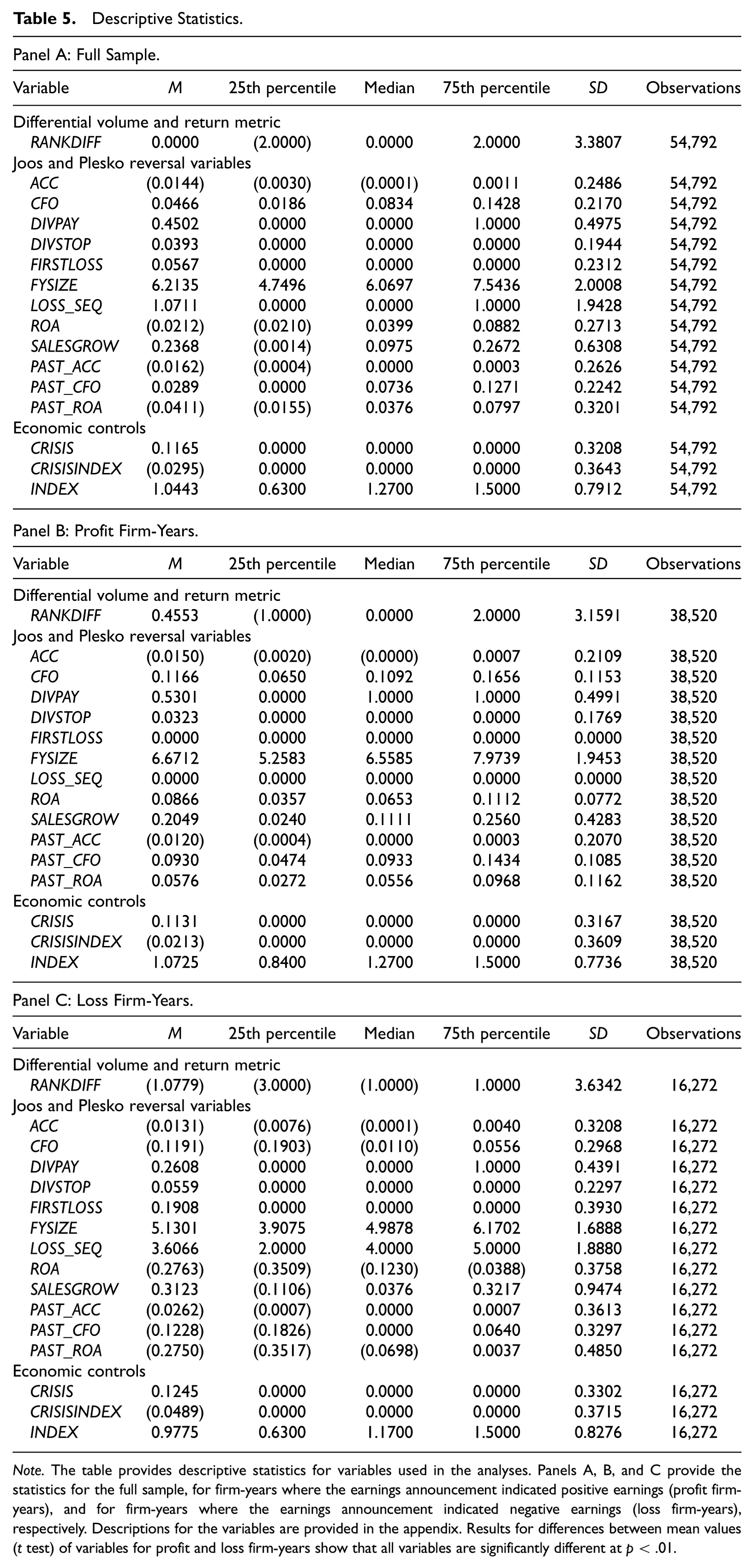
Note. The table provides descriptive statistics for variables used in the analyses. Panels A, B, and C provide the statistics for the full sample, for firm-years where the earnings announcement indicated positive earnings (profit firm-years), and for firm-years where the earnings announcement indicated negative earnings (loss firm-years), respectively. Descriptions for the variables are provided in the appendix. Results for differences between mean values (t test) of variables for profit and loss firm-years show that all variables are significantly different at p < .01.

Table 6 reports regression results. Panel A (Panel B) of Table 6 reports the results of our estimation of the first specification (second specification) of the Joos and Plesko (2005) models. We report results for both specifications of the Joos and Plesko model with and without our three economic control variables. In all specifications, RANKDIFF is positive and significant. Classifications are marginally improved when the three economic control variables (CRISIS, INDEX, and CRISIS×INDEX) are included.¹⁹ These results are consistent with our predictions that differential volume–price reactions impound information that is useful in predicting loss reversals.²⁰ The positive and significant coefficient for RANKDIFF suggests that loss announcements that generate higher volume reactions relative to price reactions are more likely to reverse subsequently. Thus, when investor disagreement is high, as implied by higher volume relative to consensus opinion reflected in price reactions, the loss is more likely to reverse.²¹

Table 6.

Prediction of Loss Reversal Using RANKDIFF.

Panel A: Joos & Plesko Model I.
	Joos & Plesko Model I
	Model A		Model B
	Coefficient	p value	Coefficient	p value
ROA	2.6709	.000	2.6965	.000
PAST_ROA	0.5639	.000	0.5183	.000
FYSIZE	0.1234	.000	0.1244	.000
SALESGROW	(0.0842)	.009	(0.0809)	.012
FIRSTLOSS	0.2982	.000	0.2948	.000
LOSS_SEQ	(0.1023)	.000	(0.1042)	.000
DIVPAY	0.2588	.000	0.2674	.000
DIVSTOP	(0.0991)	.288	(0.0838)	.371
CRISIS			0.4602	.000
INDEX			0.1582	.000
CRISIS×INDEX			(0.2494)	.000
RANKDIFF	0.0301	.000	0.0292	.000
Model statistics^a
Observations	14,526		14,526
Likelihood ratio χ²	2,534.84		2,585.70
Model p value	.0000		.0000
Pseudo-R²	.1463		.1493
Naïve classification	71.64%		71.64%
Model classification (%)	74.05		74.44
Panel B: Joos & Plesko Model II.
	Joos & Plesko Model II
	Model A		Model B
	Coefficient	p value	Coefficient	p value
CFO	3.4875	.000	3.5135	.000
PAST_CFO	0.7683	.000	0.6923	.000
ACC	0.1203	.204	0.1185	.209
PAST_ACC	(0.1396)	.062	(0.1353)	.070
FYSIZE	0.0994	.000	0.1036	.000
SALESGROW	(0.1610)	.000	(0.1676)	.000
FIRSTLOSS	0.3425	.000	0.3391	.000
LOSS_SEQ	(0.0827)	.000	(0.0849)	.000
DIVPAY	0.2730	.000	0.2797	.000
DIVSTOP	(0.0940)	.315	(0.0768)	.365
CRISIS			0.4499	.000
INDEX			0.2094	.000
CRISIS×INDEX			(0.2289)	.001
RANKDIFF	0.0331	.000	0.0321	.000
Model statistics^b
Observations	14,526		14,526
Likelihood ratio χ²	2,715.58		2,761.01
Model p value	.0000		.0000
Pseudo-R²	.1568		.1594
Naïve classification (%)	71.64		71.64
Model classification (%)	74.54		74.64

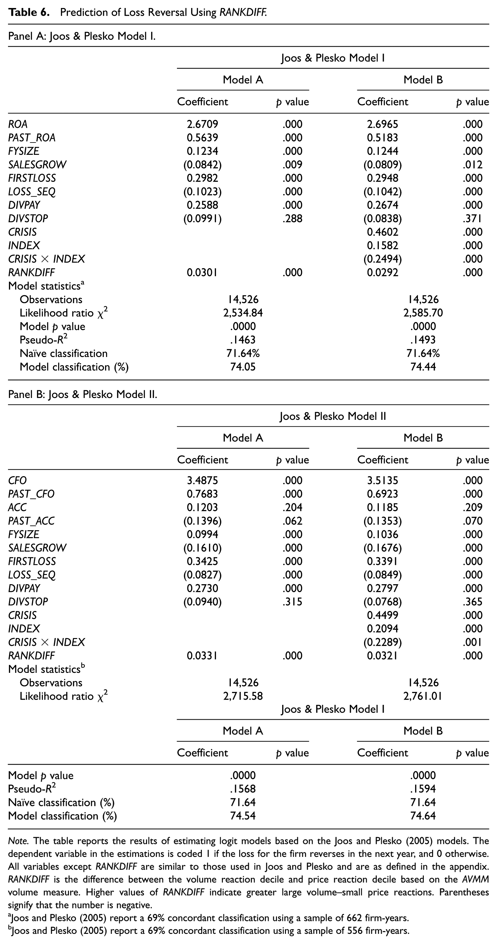
Note. The table reports the results of estimating logit models based on the Joos and Plesko (2005) models. The dependent variable in the estimations is coded 1 if the loss for the firm reverses in the next year, and 0 otherwise. All variables except RANKDIFF are similar to those used in Joos and Plesko and are as defined in the appendix. RANKDIFF is the difference between the volume reaction decile and price reaction decile based on the AVMM volume measure. Higher values of RANKDIFF indicate greater large volume–small price reactions. Parentheses signify that the number is negative.

Joos and Plesko (2005) report a 69% concordant classification using a sample of 662 firm-years.

Joos and Plesko (2005) report a 69% concordant classification using a sample of 556 firm-years.

Results of additional specification tests are reported in Table 7. Summary results for the regressions in Table 6 for RANKDIFF are included for ease of comparison and to evaluate if the predictive power of RANKDIFF is attributable solely to volume or price reaction. Table 7 reports the results of two additional regressions for each model specification where we add RANK_VOL and RANK_RET separately.

Table 7.

Prediction of Loss Reversal Using Differential Price–Volume Reaction: Decomposition of RANKDIFF.

	Model I			Model II
	Variables added to Joos & Plesko - Model I			Variables added to Joos & Plesko - Model II
	RANK_VOL	RANK_RET	RANKDIFF	RANK_VOL	RANK_RET	RANKDIFF
Model performance
Observations	14,526	14,526	14,526	14,526	14,526	14,526
Naïve correct (%)	71.64	71.64	71.64	71.64	71.64	71.64
Model correct (%)	74.16	74.39	74.44	74.45	74.62	74.64
Improvement (%)	3.52	3.84	3.91	3.92	4.16	4.19
Likelihood ratio χ²	2,571.33	2,565.34	2,585.70	2,740.62	2,743.64	2,761.01
Significance	.0000	.0000	.0000	.0000	.0000	.0000
Pseudo-R² (%)	14.84	14.81	14.93	15.82	15.84	15.94
Significance of added variable
RANK_VOL	.000			.003
RANK_RET		.011			.001
RANKDIFF			.000			.000

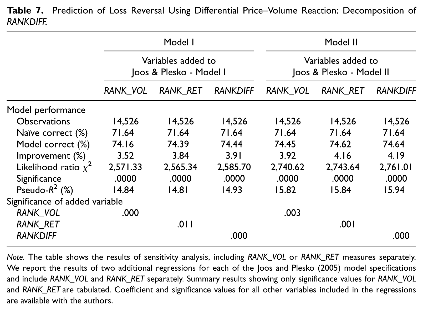
Note. The table shows the results of sensitivity analysis, including RANK_VOL or RANK_RET measures separately. We report the results of two additional regressions for each of the Joos and Plesko (2005) model specifications and include RANK_VOL and RANK_RET separately. Summary results showing only significance values for RANK_VOL and RANK_RET are tabulated. Coefficient and significance values for all other variables included in the regressions are available with the authors.

In both models, the estimations including RANK_VOL or RANK_RET produce model fit statistics and classification percentages superior to that of the base estimation. That is, trading volume reaction and price reaction metrics each separately have predictive power in predicting loss reversals.²² Thus, the predictive power of the model also improves marginally with the inclusion of these variables. Of particular interest to our study is to evaluate whether inclusion of a metric that captures the combination of differential volume and price reactions (i.e., RANKDIFF) is incrementally beneficial to considering either one separately for predicting loss reversals. Our results show that a measure based on the joint consideration (i.e., RANKDIFF) of volume and price reactions is superior to the use of only price or volume separately when predicting reversals.²³

Consensus or disagreement around loss announcements

Our results show a positive coefficient on RANKDIFF relative to loss reversals. RANKDIFF is computed as RANK_VOL−RANK_RET and is constructed such that RANKDIFF is positive where the rank of volume is larger than the rank of return. Therefore, the positive coefficient on RANKDIFF in our reversal model indicates that reversal is likely where RANK_VOL > RANK_RET. Our finding of a positive coefficient on RANKDIFF does not, however, unambiguously inform us as to whether we are observing a disaggregation of beliefs (high volume–low price) regarding a reversal or a consensus of no reversal (low volume–high price). We conduct additional analyses to answer this question.

In our first additional test, we separate RANKDIFF into positive (PRANKDIFF) and negative (NRANKDIFF). When RANKDIFF is positive, PRANKDIFF takes the value of RANKDIFF and is assigned the value of 0 otherwise. In a similar fashion, when RANKDIFF is negative, NRANKDIFF takes the value of RANKDIFF and is assigned the value of 0 otherwise. Our design of these two new variables is such that PRANKDIFF+NRANKDIFF = RANKDIFF. This design is an unrestricted model, in that we allow different coefficients to be estimated on the two segments of RANKDIFF. We estimate both reversal models (J&P Model I and J&P Model II) substituting PRANKDIFF and NRANKDIFF in place of RANKDIFF. Significance on PRANKDIFF would suggest that the power of RANKDIFF was in identifying disaggregated beliefs, and significance on NRANKDIFF would suggest that RANKDIFF is useful in identifying consensus of a secondary loss. Table 8 shows that the estimated coefficients on both PRANKDIFF and NRANKDIFF are positive and significant at conventional levels in both reversal models. In addition, the proportion of cases correctly classified is qualitatively identical to the prior results. Model performance is comparable with the earlier models.

Table 8.

Additional Tests: RANKDIFF Classified by Sign: Prediction of Loss Reversal Using PRANKDIFF and NRANKDIFF.

	J&P Model I		J&P Model II
	Coefficient	p value	Coefficient	p value
ROA	2.6937	.000
PAST_ROA	0.5186	.000
CFO			3.5131	.000
PAST_CFO			0.6962	.000
ACC			0.1213	.209
PAST_ACC			(0.1342)	.091
FYSIZE	0.1242	.000	0.1033	.069
SALESGROW	(0.0810)	.000	(0.1665)	.000
FIRSTLOSS	0.2946	.000	0.3380	.000
LOSS_SEQ	(0.1041)	.000	(0.0846)	.000
DIVPAY	0.2670	.000	0.2790	.000
DIVSTOP	(0.0833)	.374	(0.0766)	.417
CRISIS	0.4609	.000	0.4526	.000
INDEX	0.1587	.000	0.2025	.000
CRISIS×INDEX	(2.5163)	.000	(0.2391)	.000
PRANKDIFF ^a	0.0247	.042	0.0313	.026
NRANKDIFF ^a	0.0353	.000	0.0445	.000
Model statistics
Observations	14,526		14,526
Likelihood ratio χ²	2,786.04		2,761.75
Model p value	.0000		.0000
Pseudo-R²	.1493		.1594
Naïve classification (%)	71.64		71.64
Model classification (%)	74.43		74.60

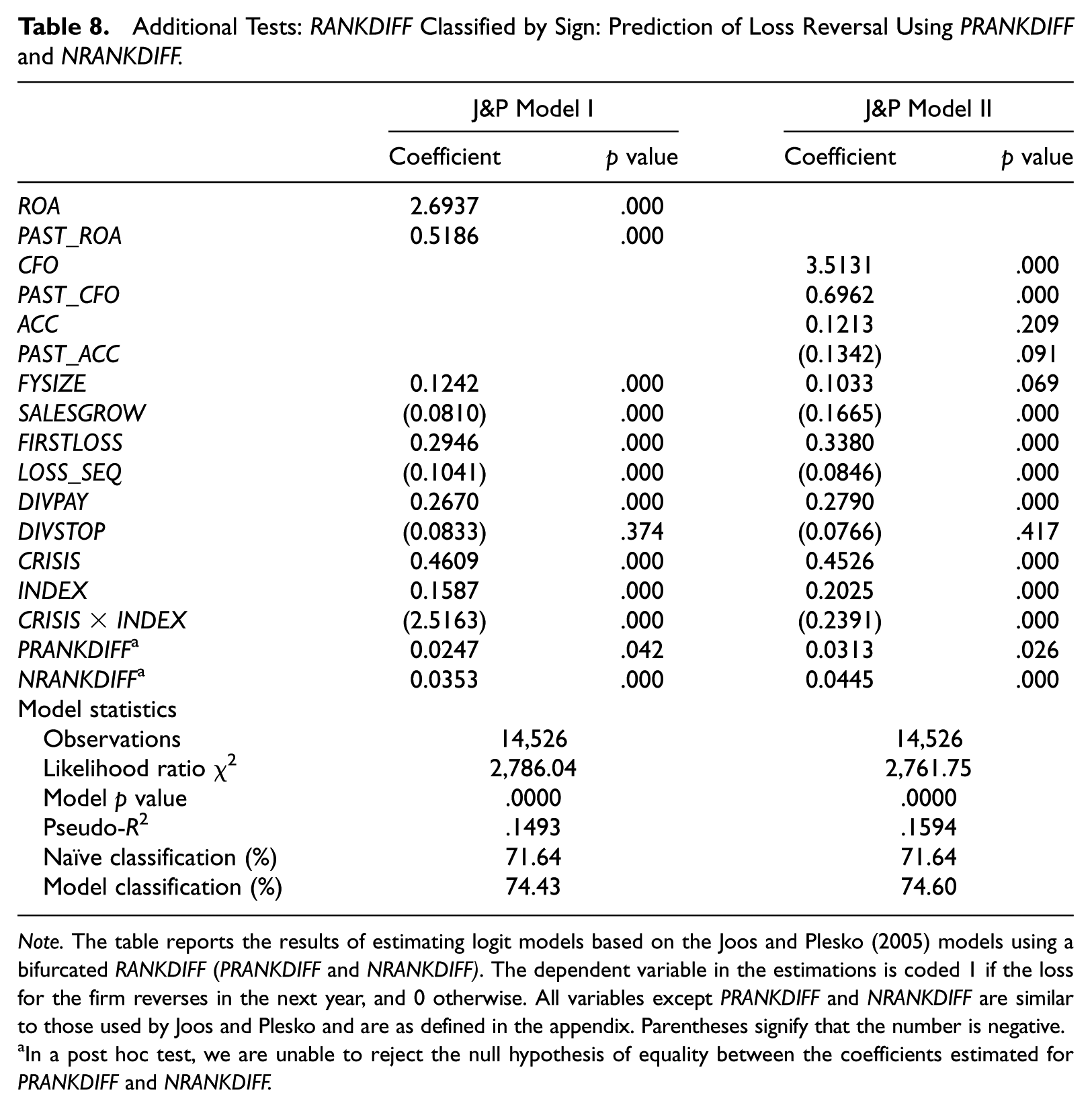
Note. The table reports the results of estimating logit models based on the Joos and Plesko (2005) models using a bifurcated RANKDIFF (PRANKDIFF and NRANKDIFF). The dependent variable in the estimations is coded 1 if the loss for the firm reverses in the next year, and 0 otherwise. All variables except PRANKDIFF and NRANKDIFF are similar to those used by Joos and Plesko and are as defined in the appendix. Parentheses signify that the number is negative.

In a post hoc test, we are unable to reject the null hypothesis of equality between the coefficients estimated for PRANKDIFF and NRANKDIFF.

By definition, our variable PRANKDIFF has positive values for observations with higher volume reactions relative to price reactions. The positive coefficient on PRANKDIFF suggests that higher levels of disaggregation of beliefs are associated with an increased probability of loss reversal. In the case of NRANKDIFF, which by our definition has negative values, the positive coefficient indicates that a lower level of volume reaction concurrent with higher level of price reaction (indicating stronger consensus) is associated with a lower probability of reversals, that is, as price reactions increase relative to volume, the probability of reversal goes down. In addition, for a given price reaction level, as volume increases the probability of reversal also increases.²⁴

Discussion and Conclusion

Our study provides an examination of differential volume–price reactions around earnings loss announcements. We find that the differential volume–price reaction around loss announcements contains information regarding the future profitability of loss firms. Where price reflects the market consensus, trading volume captures the strength of that consensus across all market participants. We compute the differential volume–price reaction metric (RANKDIFF) as the decile rank of abnormal trading volume less the decile rank of abnormal return. By comparing our variable of interest between profit and loss firms, we find that approximately 25% (16%) of loss earnings announcements (profit earnings announcements) generate either large volume–small price or small volume–large price changes. Loss firms that report a subsequent loss (profit) exhibit large volume–small price or small volume–large price in approximately 26% (21%) of the cases.

We classify abnormal volume and price reactions to negative earnings announcements into deciles and identify their difference as a measure, RANKDIFF. When RANKDIFF is positive, that is, when there are large volume reactions relative to smaller price reactions, theory suggests that there is significant disagreement among investors. The significant positive coefficient on PRANKDIFF in Table 8 suggests that a one-period-ahead loss reversal is more likely when abnormal volume is large relative to abnormal return. When there is consensus of beliefs, that is, when there are small volume reactions relative to larger price reactions, the significant positive coefficient on NRANKDIFF in Table 8 suggests that there is a lower probability of loss reversals. Of the 14,526 loss firms in our sample, our models correctly classify between 74.05% and 74.64% of the cases, and compare favorably with the naïve classification of 71.64%. Our results demonstrate that the joint consideration of trading volume and price reactions surrounding earnings announcements is superior in terms of predictive ability as compared with using measures based solely on volume or price.

We show that a metric which incorporates both volume and price reactions provides better insights regarding future profitability than using either volume or price measures alone. These results suggest that trading volume and return measures individually and jointly have predictive ability. For each measure, the correct classification of loss firm reversal in the next period is improved when RANKDIFF is included in the reversal model. Our results contribute both to the literature on volume–price reactions to firm-specific announcements and to the literature relating to loss reversals.

Footnotes

Appendix

Variable Definitions.

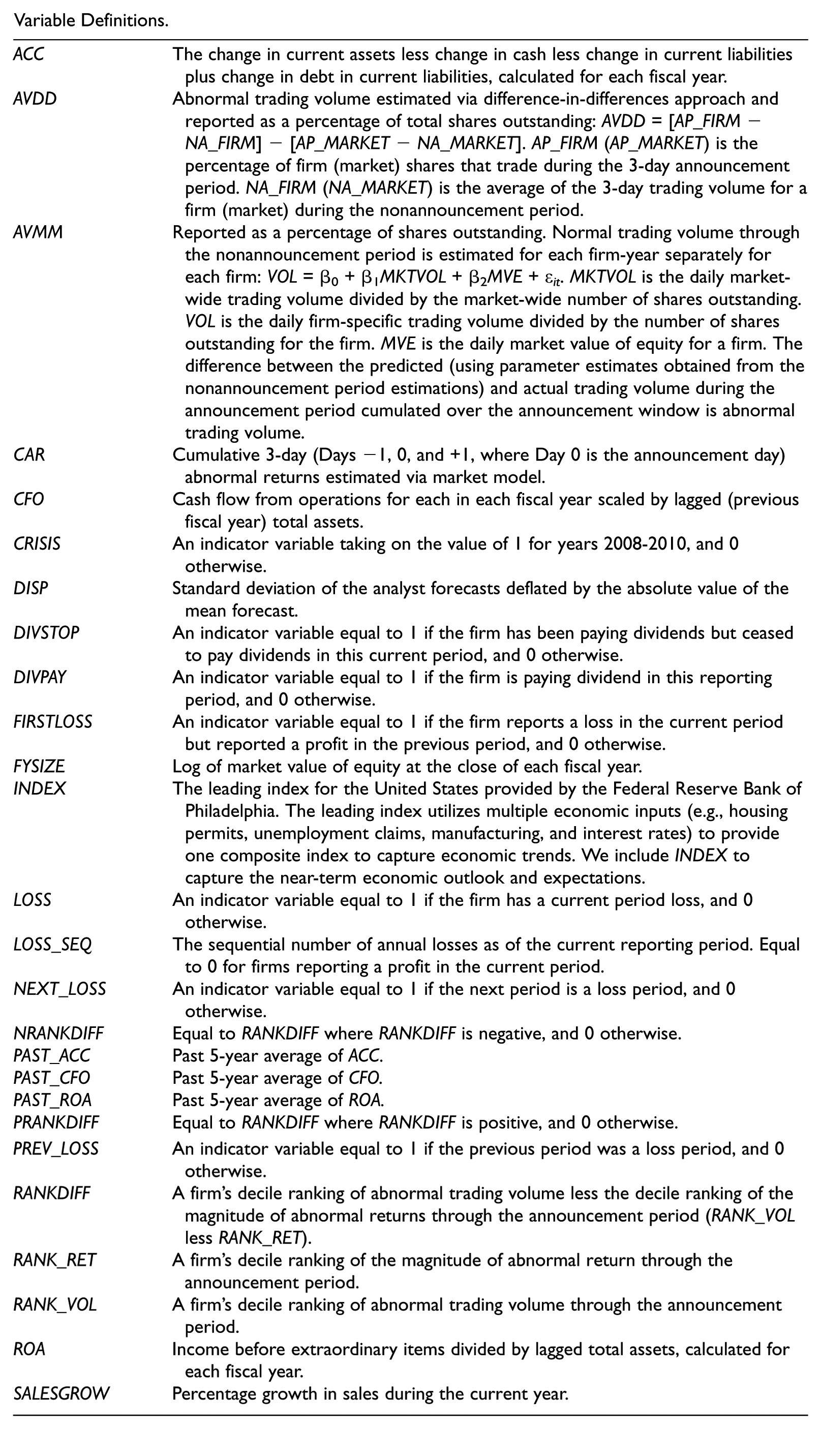
ACC	The change in current assets less change in cash less change in current liabilities plus change in debt in current liabilities, calculated for each fiscal year.
AVDD	Abnormal trading volume estimated via difference-in-differences approach and reported as a percentage of total shares outstanding: AVDD = [AP_FIRM−NA_FIRM] − [AP_MARKET−NA_MARKET]. AP_FIRM (AP_MARKET) is the percentage of firm (market) shares that trade during the 3-day announcement period. NA_FIRM (NA_MARKET) is the average of the 3-day trading volume for a firm (market) during the nonannouncement period.
AVMM	Reported as a percentage of shares outstanding. Normal trading volume through the nonannouncement period is estimated for each firm-year separately for each firm: VOL = β₀+β₁MKTVOL+β₂MVE+ϵ_it. MKTVOL is the daily market-wide trading volume divided by the market-wide number of shares outstanding. VOL is the daily firm-specific trading volume divided by the number of shares outstanding for the firm. MVE is the daily market value of equity for a firm. The difference between the predicted (using parameter estimates obtained from the nonannouncement period estimations) and actual trading volume during the announcement period cumulated over the announcement window is abnormal trading volume.
CAR	Cumulative 3-day (Days −1, 0, and +1, where Day 0 is the announcement day) abnormal returns estimated via market model.
CFO	Cash flow from operations for each in each fiscal year scaled by lagged (previous fiscal year) total assets.
CRISIS	An indicator variable taking on the value of 1 for years 2008-2010, and 0 otherwise.
DISP	Standard deviation of the analyst forecasts deflated by the absolute value of the mean forecast.
DIVSTOP	An indicator variable equal to 1 if the firm has been paying dividends but ceased to pay dividends in this current period, and 0 otherwise.
DIVPAY	An indicator variable equal to 1 if the firm is paying dividend in this reporting period, and 0 otherwise.
FIRSTLOSS	An indicator variable equal to 1 if the firm reports a loss in the current period but reported a profit in the previous period, and 0 otherwise.
FYSIZE	Log of market value of equity at the close of each fiscal year.
INDEX	The leading index for the United States provided by the Federal Reserve Bank of Philadelphia. The leading index utilizes multiple economic inputs (e.g., housing permits, unemployment claims, manufacturing, and interest rates) to provide one composite index to capture economic trends. We include INDEX to capture the near-term economic outlook and expectations.
LOSS	An indicator variable equal to 1 if the firm has a current period loss, and 0 otherwise.
LOSS_SEQ	The sequential number of annual losses as of the current reporting period. Equal to 0 for firms reporting a profit in the current period.
NEXT_LOSS	An indicator variable equal to 1 if the next period is a loss period, and 0 otherwise.
NRANKDIFF	Equal to RANKDIFF where RANKDIFF is negative, and 0 otherwise.
PAST_ACC	Past 5-year average of ACC.
PAST_CFO	Past 5-year average of CFO.
PAST_ROA	Past 5-year average of ROA.
PRANKDIFF	Equal to RANKDIFF where RANKDIFF is positive, and 0 otherwise.
PREV_LOSS	An indicator variable equal to 1 if the previous period was a loss period, and 0 otherwise.
RANKDIFF	A firm’s decile ranking of abnormal trading volume less the decile ranking of the magnitude of abnormal returns through the announcement period (RANK_VOL less RANK_RET).
RANK_RET	A firm’s decile ranking of the magnitude of abnormal return through the announcement period.
RANK_VOL	A firm’s decile ranking of abnormal trading volume through the announcement period.
ROA	Income before extraordinary items divided by lagged total assets, calculated for each fiscal year.
SALESGROW	Percentage growth in sales during the current year.

Acknowledgements

We acknowledge helpful comments and suggestions from Christo Karuna, Michael Neel, and seminar participants at the University of Houston. Our thanks are also due to an anonymous reviewer, the Associate Editor Suresh Radhakrishnan, and the Editor Bharat Sarath for their insightful guidance and comments.

Authors’ Note

Data are available from public sources identified in the text.

Declaration of Conflicting Interests

The author(s) declared no potential conflicts of interest with respect to the research, authorship, and/or publication of this article.

Funding

The author(s) received no financial support for the research, authorship, and/or publication of this article.

Notes

References

Ahmed

Schneible

Stevens

(2003). An empirical analysis of the effects of online trading on stock price and trading volume reactions to earnings announcements. Contemporary Accounting Research, 20, 413-439.

Atiase

R. K.

Bamber

(1994). Trading volume reactions to annual accounting earnings announcements: The incremental role of predisclosure information asymmetry. Journal of Accounting & Economics, 17, 309-329.

Bailey

Mao

Zhong

(2003). Regulation fair disclosure and earnings information: Market, analyst, and corporate responses. The Journal of Finance, 58, 2487-2514.

Bamber

(1986). The information content of annual earnings releases: A trading volume approach. Journal of Accounting Research, 24, 40-56.

Bamber

(1987). Unexpected earnings, firm size, and trading volume around quarterly earnings announcements. The Accounting Review, 62, 510-532.

Bamber

Barron

O. E.

Stober

T. L.

(1999). Differential interpretations and trading volume. Journal of Financial and Quantitative Analysis, 34, 369-386.

Bamber

Barron

O. E.

Stevens

D. E.

(2011). Trading volume around earnings announcements and other financial reports: Theory, research design, empirical evidence, and directions for future research. Contemporary Accounting Research, 28, 431-471.

Bamber

Cheon

(1995). Differential price and volume reactions to accounting earnings announcements. The Accounting Review, 70, 417-441.

Banerjee

Kremer

(2010). Disagreement and learning: Dynamic patterns of trade. The Journal of Finance, 65, 1269-1302.

10.

Barron

(1995). Trading volume and belief revisions that differ among individual analysts. The Accounting Review, 70, 581-597.

11.

Barron

Byard

(2010). Earnings announcement disclosures that spur differential interpretations (Working paper). State College: Pennsylvania State University.

12.

Barron

Harris

Stanford

(2005). Evidence that investors trade on private event-period information around earnings announcements. The Accounting Review, 80, 403-421.

13.

Barron

Schneible

Stevens

(2009). What do we really know about the firm size effect on trading volume reactions to earnings announcement? A re-examination and extension (Working paper). State College: Pennsylvania State University.

14.

Beaver

(1968). The information content of annual earnings announcements [Selected studies]. Journal of Accounting Research, 6, 67-92.

15.

Cochrane

(2007). Efficient markets today (Talk at Conference of Chicago Economics). Retrieved from http://chicagoboothalumniclub.org/content.aspx?page_id=87&club_id=507662&item_id=144719

16.

Collins

D. W.

Pincus

Xie

(1999). Equity valuation and negative earnings: The role of book value of equity. The Accounting Review, 74, 29-61.

17.

Cready

Hurtt

(2002). Assessing investor response to information events using return and volume metrics. The Accounting Review, 77, 891-909.

18.

Darrough

(2007). Valuation of loss firms in a knowledge-based economy. Review of Accounting Studies, 12, 61-93.

19.

Dhaliwal

D. S.

Kaplan

S. E.

Laux

R. C.

Weisbrod

(2012). The information content of tax expense for firms reporting losses. Journal of Accounting Research, 51, 135-164.

20.

Franzen

Radhakrishnan

(2009). The value relevance of R&D across profit and loss firms. Journal of Accounting and Public Policy, 28, 16-32.

21.

Garfinkel

J. A.

(2009). Measuring investors’ opinion divergence. Journal of Accounting Research, 47, 1317-1348.

22.

Garfinkel

J. A.

Sokobin

(2006). Volume, opinion divergence, and returns: A study of post-earnings announcement drift. Journal of Accounting Research, 44, 85-112.

23.

Gow

I. D.

Ormazabal

Taylor

D. J.

(2010). Correcting for cross-sectional and time-series dependence in accounting research. The Accounting Review, 85, 483-512.

24.

Harris

Raviv

(1993). Differences of opinion make a horse race. Review of Financial Studies, 6, 473-506.

25.

Hayn

(1995). The information content of losses. Journal of Accounting & Economics, 20, 125-153.

26.

Jan

(1995). The role of negative earnings in the valuation of equity stocks (Working paper). New York: New York University.

27.

Jiang

Stark

A. W.

(2011). Accounting and economic determinants of loss reversals (Working paper). Retrieved from https://www.researchgate.net/publication/228270848_Accounting_and_Economic_Determinants_of_Loss_Reversals

28.

Joos

Plesko

G. A.

(2005). Valuing loss firms. The Accounting Review, 80, 847-870.

29.

Kandel

Pearson

(1995). Differential interpretation of public signals and trade in speculative markets. Journal of Political Economy, 103, 831-872.

30.

Karpoff

(1986). A theory of trading volume. The Journal of Finance, 41, 1069-1087.

31.

Kiger

(1972). An empirical investigation of NYSE volume and price reactions to the announcement of quarterly earnings. Journal of Accounting Research, 10, 113-128.

32.

Kim

Verrecchia

(1991a). Market reaction to anticipated announcements. Journal of Financial Economics, 30, 273-309.

33.

Kim

Verrecchia

(1991b). Trading volume and price reactions to public announcements. Journal of Accounting Research, 29, 302-321.

34.

Klein

Marquardt

C. A.

(2006). Fundamentals of accounting losses. The Accounting Review, 81, 179-206.

35.

Landsman

Maydew

(2002). Has the information content of quarterly earnings announcements declined in the past three decades?Journal of Accounting Research, 40, 797-808.

36.

Leone

A. J.

Minutti-Meza

Wasley

C. E.

(2014). Influential observations and inference in accounting research (Working paper). University of Miami and University of Rochester. Retrieved from http://ssrn.com/abstract=2407967

37.

K. K.

(2011). How well do investors understand loss persistence?Review of Accounting Studies, 16, 630-667.

38.

Milgrom

Stokey

(1982). Information, trade and common knowledge. Journal of Economic Theory, 26, 17-27.

39.

Morse

(1981). Price and trading volume reaction surrounding earnings announcements: A closer examination. Journal of Accounting Research, 19, 374-383.

40.

Neter

Wasserman

(1974). Applied linear statistical models. Homewood, IL: Richard D. Irwin.

41.

Neter

Wasserman

Kutner

M. A.

(1983). Applied linear regression models. Homewood, IL: Richard D. Irwin.

42.

Shalen

(1993). Volume, volatility, and the dispersion of beliefs. Review of Financial Studies, 6, 405-434.

43.

Utama

Cready

(1997). Institutional ownership, differential predisclosure precision and trading volume at announcement dates. Journal of Accounting & Economics, 24, 129-150.