Measuring the Persistency of Earnings Components: Applications of the VAR Model to Long-Run Japanese Data

Abstract

This study investigates the time-series properties of accounting earnings and their components. We propose a new measure of earnings persistency in accordance with the vector autoregressive (VAR) model–linked earnings and stock returns. As a preliminary analysis, we estimate the first-order autocorrelations and test the stationarity of five variables: earnings, cash flows from operations, total accruals, current accruals, and noncurrent accruals. We then confirm that earnings and noncurrent accruals have a more persistent time-series than cash flows and current accruals. Next, we formulate and estimate the first-order autoregressive model composed of the three variables of utmost interest to accounting researchers, namely, cash flows, current accruals, and noncurrent accruals, and explore how future predictions of these three earnings components are affected by unit impulse shocks. Given the results of the impulse response function analysis, we forecast changes in stock prices based on future innovations of these components, finding that a 1% unit shock in the earnings components affects stock prices by 2% to 2.5%. Finally, we are able to demonstrate excess returns by using the portfolio formation method based on our measure of persistence.

Keywords

persistency of earnings vector autoregressive model accounting accruals earnings innovations impulse response functions

Introduction

A large number of empirical studies have tested the mispricing phenomena obtained from the accruals components of earnings (e.g., Sloan, 1996; Xie, 2001). These studies argue that the market misjudges implications from accounting accruals.¹ Most of these studies have used the pooled sample estimation method. However, Teets and Wasley (1996) demonstrate that earnings response coefficients estimated using pooled data are downwardly biased for U.S. data. Moreover, Chan, Jegadeesh, and Sougiannis (2004) report, again for U.S. data, that the predictability of future earnings can be significantly improved by using the vector autoregressive (VAR) model. Accordingly, we focus here on the time-series properties of accounting numbers and investigate the information on accounting accruals compared with cash flow information and earnings numbers for a sample of Tokyo Stock Exchange–listed firms.

The proposed research framework is novel in four ways. First, we estimate the detailed stochastic processes of accounting numbers at the individual firm level and conduct the Dickey–Fuller (DF) test (see Dickey & Fuller, 1979). Second, we use a VAR model approach to explicitly consider the interactions among the earnings components. Third, based on the estimates of our VAR model, we forecast stock price changes based on the future innovations of these components with stock valuation functions. For this purpose, we use the spectral radius concept to measure persistency as well as an extension of the valuation function originally proposed by Kormendi and Lipe (1987). Finally, by using the portfolio formation method, we construct 30 persistency- and earnings component-ranked portfolios, confirming that some of the abnormal returns from the accruals anomaly may be explained by the overvaluation or undervaluation of the persistency of individual stocks by investors.

The organization of the remainder of the article is as follows. “Forecasting Accounting Earnings by Using a VAR Model” section discusses the relationship between the efficient market hypothesis and accounting reports based mainly on previous U.S. and Japanese evidence. “Accounting Earnings and Their Components” section defines the components of the accounting accruals used in this study. “Method and Data” section explains our estimation methods and motivates our research methodology. “Empirical Results” section describes our data and reports the basic findings. In “Persistency Measures From VAR(1)” section, we apply impulse response analysis to compute our new measures of persistency. After discussing the features of our persistency measures, we also present the results of the stock return analysis, showing that some of the accruals anomaly can be explained by investors incorrectly recognizing persistency. “Conclusion” section concludes the manuscript.

Forecasting Accounting Earnings by Using a VAR Model

In most pioneering works on the accruals anomaly, univariate first-order autoregressive models have been used to predict future accounting earnings (Sloan, 1996; Xie, 2001). However, those univariate forecasting models disregard the interactions among earnings components. As Chan et al. (2004) point out, the predictability of future earnings can be improved significantly by using the VAR model, which explicitly takes into consideration the time-series interactions among earnings components.² In an analogous way, Nam, Brochet, and Ronen (2012) show that the power of accruals to predict future cash flows varies significantly across firms and that mispricing associated with accruals only occurs in firms where accruals are poor predictors of future cash flows.

In the current study, based on the first-order VAR model, which can explicitly take into account the interactions among earnings components, we propose a new measure of “earnings persistency,” which is measured using the spectral radius of the slope coefficient matrix as well as the present value of the earnings revision derived from the VAR model. Then, we examine stock price responses from the impulse shocks of earnings components and show that some of the accruals anomaly can be explained by investors incorrectly recognizing the persistency of earnings components.

Accounting Earnings and Their Components

For income numbers, we use net income after-tax wherein extraordinary gains and losses are added back (earnings before extraordinary items [EBEI]) as a base income number for our analysis. This income concept, so-called “current earnings after tax,” is the bottom line net income number that financial analysts in Japan often follow and predict. This net income number contains the performance of the financing decisions of firms except for items of other comprehensive income, which are directly charged to the equity account as dirty surplus in accordance with Japanese accounting standards.

The earnings number, EBEI, can be decomposed into cash flows from operations (CFO) and total accruals (ACC). We use total assets at the beginning of the period as a common deflator to construct all the variables. In addition, since cash flow statements were not available in Japan before 2000, we compute the four accruals components, ΔCOA, ΔCOL, ΔNCOL, and DEPR, from the balance sheet and income statements in individual unconsolidated financial statements as,

Δ COA = (changes in current assets - changes in cash and deposits) .

Δ COL = - (changes in current liabilities - changes in financing items) .

\begin{matrix} Δ NCOL = - (changes in loss allowances for accounts receivable \\ + changes in reserve for bonus payable and salary payable \\ + changes in short - term reserve accounts \\ + changes in allowance for future retirement bonus \\ + changes in long - term reserve accounts \\ + changes in amortization) . \end{matrix}

DEPR = - (depreciation) .

The changes in financing items in Equation 2 are composed of changes in short-term borrowing, changes in outstanding commercial papers, changes in long-term debt due within 1 year, and straight bonds and convertible bonds due within 1 year. Note that ΔCOL, ΔNCOL, and DEPR are defined as negative numbers throughout the article; hence, ACC become larger (smaller) as these numbers become larger (smaller).

Using the notations defined in Equations 1 to 4, current accruals (CACC), noncurrent accruals (NCACC), and ACC are defined as,

\begin{matrix} CACC = Δ COA + Δ COL \\ NCACC = Δ NCOL + DEPR \\ ACC = CACC + NCACC . \end{matrix}

Because ACC are the gaps between accounting earnings (EBEI) and CFO, the latter is defined as,

CFO = EBEI - ACC .

The variables in Equation 6, EBEI, ACC, and CFO, are deflated by total assets at the beginning of the period.

Method and Data

Time-Series Property of the Accounting Earnings Components

Although U.S. data offer ample evidence for the time-series properties of the accounting numbers, few such data exist for Japanese firms. In this article, we therefore present evidence of the estimated first-order autocorrelations using an ordinary least squares (OLS) estimation, and conduct the DF test and Kwiatkowski, Phillips, Schmidt, and Shin’s (1992) unit root test (KPSS test hereafter) since both assume that time-series X_t has drift but without a deterministic trend:

X_{t} = a + ρ \cdot X_{t - 1} + u_{t} .

We use a sample that covers at least 10 consecutive years of observations. In the above equation, the u_ts are assumed to be distributed with Gaussian white noise and the initial value X₀ is assumed to be zero. When the true ρ is close to 1, the estimated ρ from the OLS regression is underestimated (Harvey, 1981). Accordingly, in the case where the true ρ equals 1, the distributions of ρ are not well defined in a normal manner, and alternative DF tests are called for, in which the numerator is the chi-square distributed variable and the denominator is the normally distributed variable.

If the null hypothesis of the existence of a unit root in the DF test is not rejected, the model becomes a random walk model with drift; hence, the accounting numbers are highly persistent in the sense of Kormendi and Lipe (1987).³ On the contrary, if the null hypothesis of a unit root in the DF test is rejected, it is called less persistent. However, accounting earnings and their components must be assumed to be stationary when we correctly apply autoregression or VAR models to investigate their time-series behavior. Thus, we conduct the KPSS test in which the null hypothesis is the stationarity of the series (Kwiatkowski et al., 1992). If the null hypothesis of a unit root in the DF test is rejected, while the null hypothesis of stationarity in the KPSS test is not, for all the earnings components, we can safely apply a VAR(1) model as a base for the analysis.

VAR Model for Earnings Forecasting

In the framework proposed by Sloan (1996), it is assumed that earnings are a solely value-relevant variable and that earnings in the next year can be optimally forecasted using the univariate first-order autoregressive model. However, as noted by Chan et al. (2004), the univariate autoregressive model cannot approximate the market expectations of earnings. Therefore, the predictability of future earnings can be improved by using a VAR model, which explicitly takes into consideration the interactions among earnings components over time. With this framework, we propose a new persistency measure of earnings and a test for rational pricing based on the VAR model.

Because the number of annual observations of the accounting figures of a particular firm is limited, using VAR models with more than one lag is not possible. Accordingly, we adopt a tractable multivariate time-series model, namely, the following first-order VAR model:

\begin{matrix} Y_{t} = (\begin{matrix} CF O_{t} \\ CAC C_{t} \\ NCAC C_{t} \end{matrix}) = (\begin{matrix} γ_{01} \\ γ_{02} \\ γ_{03} \end{matrix}) + (\begin{matrix} γ_{11} & γ_{12} & γ_{13} \\ γ_{21} & γ_{21} & γ_{23} \\ γ_{31} & γ_{32} & γ_{33} \end{matrix}) (\begin{matrix} CF O_{t - 1} \\ CAC C_{t - 1} \\ NCAC C_{t - 1} \end{matrix}) + (\begin{matrix} v_{1 t} \\ v_{2 t} \\ v_{3 t} \end{matrix}) \\ = Γ_{0} + Γ Y_{t - 1} + v_{t} . \end{matrix}

To investigate the effects of past earnings components on future ones, we use impulse response analysis, which is an often-used approach to examine the behavior of dynamic models in engineering and macroeconomics. The impulse response used in this study is defined as the reaction of the system of Equation 8 in response to the changes in earnings components.

The resulting impulse response functions in Equation 8 can then trace the effects of a unit shock on one of the earnings components onto the other components in the VAR. Because we use a first-order VAR model, the relation between Y_t and the k period lead variable Y_t_+k is found in Equation 9. Here, we observe that the unit shock to Y_t_-1 is conveyed through matrix $Γ^{k}$ and that the impulse response function is identical to this matrix:

\begin{matrix} Y_{t} = Γ_{0} + Γ Y_{t - 1} + v_{t} \\ Y_{t + k} = (I + \sum_{j = 1}^{k} Γ^{j - 1}) Γ_{0} + Γ^{k + 1} Y_{t - 1} + (v_{t + k} + \sum_{j = 1}^{k} Γ^{k} v_{t + k - j}) . \end{matrix}

Earnings Persistency and Valuation Model under VAR Specifications

Kormendi and Lipe (1987) derive the theoretical measure of earnings persistency by assuming the following three conditions. First, the univariate autoregressive model approximates the market expectations of earnings. Second, the stock price is equal to the present value of expected future cash flows to shareholders, meaning that investors can estimate the intrinsic value of equity by applying the dividend discount model. Third, changes in expected earnings are equal to changes in expected dividends to shareholders. In this study, we make the second and third assumptions. We do not use the first assumption of Kormendi and Lipe (1987) but rather replace it with an estimation of the earnings numbers predicted by our VAR(1) model. In other words, we assume that the earnings components are optimally forecasted by the vector-specified form of the VAR(1) model.

To further expand this formula, first note by definition that the sum of changes in the earnings components is equal to the change in earnings, and thus, the following equation holds:

\begin{matrix} Δ EBE I_{t} = Δ CF O_{t} + Δ CAC C_{t} + Δ NCAC C_{t} \\ = e^{t} Δ Y_{t} = e^{t} (Y_{t} - Y_{t - 1}) = e^{t} ((Γ_{0} + Γ Y_{t - 1} + ν_{t}) - (Γ_{0} + Γ Y_{t - 2} + ν_{t - 1})) \\ = e^{t} Γ Δ Y_{t - 1} + e^{t} (ν_{t} - ν_{t - 1}) \\ E (Δ EBE I_{t}) = e^{t} E (Δ Y_{t}) = e^{t} Γ E (Δ Y_{t - 1}) . \end{matrix}

In Equation 10, e denotes a three-dimensional column vector whose elements are all ones, and the superscript t denotes a transpose of a vector and a matrix.

From the second and third assumptions in Kormendi and Lipe (1987), the expected change in stock price, ΔP_t, must be equal to the present value of future changes in earnings. By evaluating the expressions below, we can finally reach the valuation of ΔP_t, in which the present value of the expected change in the stock price is equal to the revisions of the earnings forecasts:

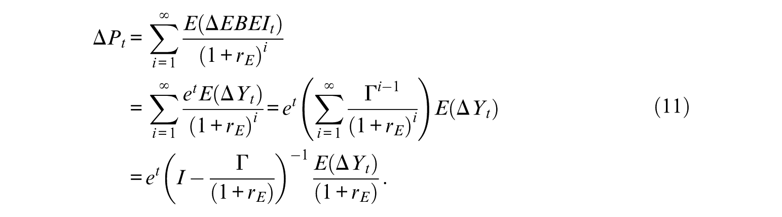
\begin{matrix} Δ P_{t} = \sum_{i = 1}^{\infty} \frac{E (Δ EBE I_{t})}{{(1 + r_{E})}^{i}} \\ = \sum_{i = 1}^{\infty} \frac{e^{t} E (Δ Y_{t})}{{(1 + r_{E})}^{i}} = e^{t} (\sum_{i = 1}^{\infty} \frac{Γ^{i - 1}}{{(1 + r_{E})}^{i}}) E (Δ Y_{t}) \\ = e^{t} {(I - \frac{Γ}{(1 + r_{E})})}^{- 1} \frac{E (Δ Y_{t})}{(1 + r_{E})} . \end{matrix}

In Equation 11, r_E denotes the cost of equity and ΔY_t the changes in the earnings components in period t. Based on this equation, we propose two alternative measures of earnings persistency: a spectral radius of matrix Γ / (1 +r_E) and a measure comparable with the present value of revision (PVR) used in Kormendi and Lipe (1987).

Our first new measure of persistence is a spectral radius, which is defined as the maximum eigenvalue of matrix Γ / (1 +r_E). That is, if spectral radius ρ is greater than 1, at least one element in (Γ / (1 +r_E))ⁱ does not stay bounded as time horizon i increases. In this case, the expected changes in stock price ΔP_t will not converge to a finite value. From another angle, the fact that spectral radius ρ is close to 1 means that innovation in the earnings components is closer to the permanent component of the stochastic process, where earnings can be termed more “persistent.” Therefore, this spectral radius of matrix Γ / (1 +r_E) can be regarded as a new measure of earnings persistence whenever future earnings can be optimally forecasted using the VAR(1) model.

Our second measure of persistence is the three-dimensional vector, defined in Equation 12, which is directly comparable with the PVR measure used in Kormendi and Lipe (1987):

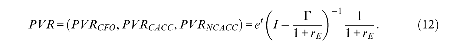
PVR = (PV R_{CFO}, PV R_{CACC}, PV R_{NCACC}) = e^{t} {(I - \frac{Γ}{1 + r_{E}})}^{- 1} \frac{1}{1 + r_{E}} .

Comparing this equation with Equation 11 allows us to show that this PVR measure simply represents the present value of the revisions of expected future changes in earnings triggered by an impulse unit shock onto one of the earnings components. This way, based on the earnings innovations derived from our VAR model, we construct a stock price valuation model using Equations 11 and 12 and conduct empirical tests.

Empirical Results

Data

The primary source for the accounting variables of the Tokyo Stock Exchange First and Second Section firms is the NIKKEI NEEDS database supplied by NIKKEI Digital Media, Inc. The primary source for monthly return data is the NIKKEI NEEDS Daily Stock Returns Database.

For the EBEI, CFO, ACC, CACC, and NCACC variables, the top and bottom observations are winsorized at the 99.5 and 0.5 percentiles. The sampling period runs from 1978 to 2014, and the number of pooled sample observations after excluding the extreme observations is 44,048 firm years. The minimum number of yearly observations is 694 for 1978 and the maximum number is 1,618 for 2014, with an average of 1,190 firms per year.

We limit our sample to nonfinancial firms listed on the Tokyo Stock Exchange. Since the fiscal years of most Japanese firms end in March, we compute the next year’s portfolio returns starting July 1. Hence, to align calendar days, we also exclude firms whose fiscal years do not end in March, which consists of less than 10% of the sample.

Basic Observations

Table 1 reports the descriptive statistics for the pooled sample data from 1978 to 2014. We find that the mean of ACC and NCACC are both negative (−2.369 and −3.033, respectively). The estimated standard deviations of earnings (EBEI) and NCACC are relatively low (4.059 and 4.209), whereas those of both CFO and ACC are quite high (13.131 and 13.006), respectively.

Table 1.

Descriptive Statistics.

	M	SD	First quintiles	Median	Third quintiles
EBEI	2.448	4.059	0.860	2.114	3.892
CFO	4.817	13.131	1.324	4.871	8.528
ACC	−2.369	13.006	−5.789	−2.654	0.589
CACC	0.665	11.576	−2.235	0.301	3.073
NCACC	−3.033	4.209	−4.272	−2.666	−1.261

Note. The sample consists of 44,048 firm years between 1978 and 2014. Firm characteristics are defined as follows: EBEI = earnings before extraordinary items; CFO = cash flows from operations; ACC = total accruals; CACC = current accruals; NCACC = noncurrent accruals. All variables are divided by total assets at the beginning of the period.

Next, Table 2 reports the correlation matrix for earnings and their components. The correlation between CFO and ACC is negative with a very high number of –.952 for the Spearman rank correlation and an even higher value of –.836 for the Pearson correlation. The result may indicate that the higher the cash flows, the lower is earnings management behavior. The correlation between cash flows and CACC is also high at –.690 for the Spearman rank correlation while that between cash flows and NCACC is a little lower at –.396. Because the Spearman correlation between current and noncurrent accruals is almost 0 (–.038), these two components may be proxies for different accruals accounting, where the weight of current accruals is larger than that of noncurrent accruals because the former are more highly associated with total accruals (.862 vs. .397 for noncurrent accruals).

Table 2.

Correlation Matrix.

	EBEI	CFO	ACC	CACC	NCACC
EBEI		.393	.072	.138	−.124
		.000	.000	.000	.000
CFO	.185		−.836	−.690	−.396
	.000		.000	.000	.000
ACC	.125	−.952		.862	.397
	.000	.000		.000	.000
CACC	.160	−.889	.948		−.038
	.000	.000	.000		.000
NCACC	−.054	−.495	.483	.179
	.000	.000	.000	.000

Note. The sample consists of 44,048 firm years between 1978 and 2014. Firm characteristics are defined as EBEI = earnings before extraordinary items; CFO = cash flows from operations; ACC = total accruals; CACC = current accruals; NCACC = noncurrent accruals. All variables are divided by total assets at the beginning of the period. The figures in the above diagonal elements of the matrix are the Spearman rank correlations and the numbers below the diagonal elements of the matrix are the Pearson correlations. The figures shown in italics in the lower cells are the corresponding p values.

Unit Root Tests of Accounting Numbers

In the early empirical accounting literature, the word “persistency” generally meant the estimated time-series regression coefficients of candidate accounting numbers on the lagged one series of the same variable. As shown by Kormendi and Lipe (1987), if a univariate autoregressive model better approximates the market expectations of earnings, it leads us to predict that higher the earnings persistency, the larger is the influence of unanticipated changes in earnings upon stock returns.

Table 3 shows the distributions of the first-order autocorrelation coefficients of earnings, cash flows, total accruals, current accruals, and noncurrent accruals. The results suggest possible earnings persistency. For EBEI and NCACC, some of the first-order autocorrelations are high and close to 1. For example, the 90th percentiles for EBEI and NCACC are .715 and .685, respectively, much higher than those for CFO, ACC, and CACC. Accordingly, the EBEI and NCACC series are expected to be more persistent than the other three earnings components.

Table 3.

Summary Statistics of the First-Order Autocorrelation.

	EBEI	CFO	ACC	CACC	NCACC
10th percentile	.071	−.369	−.328	−.391	−.196
First quintiles	.275	−.234	−.192	−.246	−.001
Median	.457	−.071	−.018	−.088	.242
M	.425	−.065	−.014	−.084	.244
Third quintiles	.611	.091	.148	.075	.510
90th percentile	.715	.252	.316	.231	.685
Results of DF test
%H₀ rejected	70.275	96.711	95.754	97.129	80.742
Results of KPSS test
%H₀ not rejected	66.148	91.806	86.005	94.079	65.550

Note. The summary of the estimation results of the autocorrelation coefficients from 1,672 sample firms for which the time-series observations for accounting numbers were available for at least 10 consecutive years. The observation years are between 1978 and 2014. EBEI is earnings after-tax and before extraordinary items, CFO = cash flows from operations, ACC = total accruals, CACC = current accruals, and NCACC = noncurrent accruals. We conduct DF and KPSS unit root tests with drift terms. “%H₀ rejected” is the percentage of firms for which a null hypothesis of a unit root is rejected at the 5% significance level. “%H0 not rejected” is the percentage of firms for which a null hypothesis of stationarity is not rejected at the 5% significance level. DF = Dickey–Fuller; KPSS = Kwiatkowski–Phillips–Schmidt–Shin.

However, the regression coefficients of the variable on the lagged one variable are downwardly biased from 1, even when the model is a random walk (Harvey, 1981, p. 29). Hence, applying univariate time-series regression coefficients to each firm is not recommended. To assess the nature of the stochastic processes of these accounting numbers, we thus conduct DF and KPSS unit root tests with drift and without a deterministic time trend. In these tests, we set the minimum requirement for the number of annual observations for each firm sample at 10, while most of our data have 37 years of observations. Finally, 1,672 firm samples satisfy these conditions in our accounting data set.

As for EBEI, we find that in 70.275% of cases, the existence of a unit root is rejected, while in 66.148% of the cases, stationarity is not rejected at the 5% significance level (see the bottom two rows of Table 3). These results suggest that the EBEI series is the most persistent among the five series.⁴ As for NCACC, these proportions are 80.742% for the DF test and 65.550% for the KPSS test, suggesting that it is the second most persistent.

On the contrary, we find that the average values of the first-order autocorrelation coefficients for CFO, total accruals ACC, and CACC are negative and close to 0 (–.065, –.014, and –.084, respectively). Note that the mean reverting process is called “less persistent” according to the definition of Schipper and Vincent (2003), on which our interpretation is based. As for cash flows, for 96.711% of the firms, the existence of a unit root is rejected at the 5% significance level, while the null hypothesis of stationarity is not rejected for 91.806% of the firms. The proportions of the firms for which the existence of a unit root is rejected and stationarity is not rejected are thus 95.774% and 86.005% for total accruals and 97.129% and 94.079% for current accruals, respectively. In sum, we conclude that the latter three components of earnings (i.e., CFO, ACC, CACC) are more likely to follow mean reverting processes and tend to revert to their means quickly. Among these variables, the most mean reverting is current accruals. Because accounting deferral or the accruals process, particularly current accruals, has to revert itself within one period (Francis & Smith, 2005), this finding is not surprising; it also reconfirms the mechanism that works with our data for both accruals processes.⁵

An important observation in Table 3 is that the first-order autocorrelation coefficients of the earnings components have large dispersions across all firms. For example, the 10th percentile of earnings is quite low at .071, whereas the 90th percentile is quite high at .715. Indeed, we find that the degrees of persistency for each firm are quite different, suggesting that the pooling method is unsuitable in accounting research.

Persistency Measures From VAR(1)

Spectral Radius and PVR Measures of Persistence

Table 4 reports the summary statistics of the estimated spectral radius and presents values of future earnings revisions (PVRs) as defined in Equation 12. The total number of firm samples is 1,637 after removing 35 firms from the sample for which the spectral radius of the matrix $Γ / (1 + r_{E})$ was larger than 1.

Table 4.

Summary Statistics of the Persistency Measures.

	M	SD	First quintiles	Median	Third quintiles
Spectral radius	0.578	0.169	0.454	0.586	0.705
PVR_CFO	2.266	1.516	1.348	1.875	2.672
PVR_CACC	2.201	1.460	1.318	1.825	2.626
PVR_NCACC	2.487	3.575	1.078	1.940	3.287

Note. The number of firms is 1,637 after excluding the 35 firms whose spectral radius of matrix Γ / (1 +r_E) is greater than 1. The definitions of the PVR measures are provided in Equation 12. PVR = present value of revision.

We find that the average and median spectral radius values are 0.578 and 0.586, which are slightly larger than the corresponding values of the first-order correlation numbers (.425 and .457) for EBEI in a single equation AR(1) specification (see Table 3). Consequently, we infer that the forecast earnings from our VAR specifications possess similar persistency to the original earnings series, which leads us to conduct further inferences on the stock price changes triggered by changes in earnings innovations.

For the present value of impulse shocks in earnings components (PVR), the average values for PVR_CFO, PVR_CACC, and PVR_NCACC are 2.226, 2.201, and 2.487, respectively (Table 5).⁶ The results suggest that an impulse shock of 1% in the earnings components over total assets affects stock prices by 2% to 3%, while NCACC are more persistent than CFO and CACC.

Table 5.

Results of the Portfolio Formation Test.

Panel A: Average Returns From PVR_CFO- and CFO-Ranked 30 Portfolios.
	CFO1	CFO2	CFO3	CFO4	CFO5	Spr.	t value	p value
PVR-NA	1.183	1.080	1.030	0.848	0.977	0.205	0.858	.392
PVR1 (high)	0.569	0.693	0.722	0.766	0.799	−0.230	−1.099	.273
PVR2	0.725	0.646	0.930	0.733	0.732	−0.006	−0.037	.970
PVR3	0.724	0.802	0.817	0.819	0.944	−0.220	−1.023	.307
PVR4	0.751	0.713	0.809	0.812	0.745	0.006	0.035	.972
PVR5 (low)	0.766	0.830	0.730	0.764	0.550	0.216	1.113	.267
Panel B: Average Returns From PVR_CACC- and CACC-Ranked 30 Portfolios.
	CCACC1	CACC2	CACC3	CACC4	CACC5	Spr.	t value	p value
PVR-NA	0.928	1.031	0.951	0.905	1.296	−0.368	−1.679	.095
PVR1 (high)	0.648	0.586	0.641	0.742	0.913	−0.265	−1.561	.120
PVR2	0.690	0.830	0.705	0.712	0.858	−0.168	−1.115	.266
PVR3	0.769	0.776	0.830	0.713	0.883	−0.114	−0.650	.516
PVR4	0.751	0.753	0.795	0.686	0.791	−0.040	−0.250	.802
PVR5 (low)	0.646	0.715	0.669	0.904	0.859	−0.213	−1.264	.208
Panel C. Average Returns From PVR_NCACC- and NCACC-Ranked 30 Portfolios.
	NCCACC1	NCACC2	NCACC3	NCACC4	NCACC5	Spr.	t value	p value
PVR-NA	0.867	0.905	1.221	0.949	1.207	−0.340	−2.158	.032
PVR (high)	0.775	0.669	0.674	0.713	0.711	0.063	0.316	.753
PVR2	0.849	0.562	0.644	0.759	0.753	0.096	0.476	.634
PVR3	0.969	0.735	0.736	0.856	0.838	0.131	0.697	.487
PVR4	0.790	0.718	0.684	0.608	0.776	0.014	0.064	.949
PVR5 (low)	0.844	0.843	0.731	0.712	0.927	−0.083	−0.370	.712

Note. At the end of June in each year (t = 1998, . . ., 2014), all the firms listed on the Tokyo Stock Exchange are ranked by persistency measures and their corresponding earnings components. PVR = present value of revision; CFO = cash flows from operations, CACC = current accruals, and NCACC = noncurrent accruals; NA = not available. The numbers reported in each cell are the average monthly returns of the portfolio (in %) and Spr. denotes the return spreads between P1 and P5. t value denotes the test statistics from the Student t test, and p value denotes the corresponding probability values.

The dispersion of the persistency of noncurrent accruals, PVR_NCACC, is larger than that of cash flows and current accruals. Although not reported in Table 5, the estimated persistency measures of NCACC are negative in 9% (153/1,637) of cases, suggesting that an increase in noncurrent accruals decreases stock prices. Fewer than 1% of firms have negative PVRs for CFO and CACC.

Stock Return Analysis

We proposed new persistency measures of earnings components based on the VAR model described in Equation 8. As pointed out by Chan et al. (2004), the predictability of future earnings can be significantly improved by using the VAR model. Hence, investors can more precisely estimate the impact of changes in current earnings components on future stock prices using the proposed new persistency measures. Consequently, the abnormal returns from an accruals-based trading strategy may no longer be earned after controlling for the new persistency measures. Nam, Brochet, and Ronen (2012) test a similar prediction for the relationship between the explanatory power of the forecasting model and accruals anomaly. They use the portfolio formation method and show that the accruals anomaly studied by Sloan (1996) is partly related to the out-of-sample predictive ability of accruals for future cash flows.

To investigate the relationship between our persistency measure and the accruals anomaly, we also construct persistency- and earnings component-ranked portfolios. At the end of June in each year (t = 1998, . . ., 2014), we compute the PVR measures, PVR_CFO, PVR_CACC, and PVRN_CACC, using the past 20 years of data.⁷ In the first stage, the firms for which PVR_CFO is available are ranked first according to the PVR_CFO- and PVR_CFO-ranked quintile portfolios (PVR1, . . ., PVR5). We also construct a portfolio of stocks for which PVR_CFO is not available (PVR-NA). In the second stage, each of these six portfolios is subdivided into five subportfolios based on the CFO ranking. As a result, we obtain 30 PVR_CFO- and CFO-ranked portfolios ((5 + 1) × 5 = 30). In a similar way, we construct the 30 PVR_CACC- and CACC-ranked portfolios and the 30 PVR_NCACC- and NCACC-ranked portfolios. By examining the stock return behavior of these three types of two-way ranked portfolios, we shed light on the mechanism that stands behind the accruals anomaly in Japan.

Table 5 reports the average monthly returns of the portfolios generated from 1-year buy-and-hold strategy. Panel A of Table 5 summarizes the average monthly returns of the 30 PVR_CFO- and CFO-ranked portfolios. The six rows labeled PVR-NA, PVR1, . . ., PVR5 show the average monthly returns from these 30 PVR_CFO- and CFO-ranked portfolios. The signs of the return spreads (Spr.) are mixed and none is significant. These findings suggest that investors find it hard to earn abnormal returns from the trading strategies solely utilizing the information contained in cash flows.

Panel B of Table 5 shows the average returns of the 30 PVR_CACC- and CACC-ranked portfolios. The first row shows the average returns from the PVR-NA quintile portfolios of the firms for which PVR_CACC is not available. As for the PVR-NA portfolios, the return spread is very low at −0.368% (−4.416% per annum) and significant at the 10% level (p value = .095). This finding means that investors cannot correctly recognize the persistency of current accruals when sufficiently long time-series data for the estimation are not available. Because PVR_CACC cannot be estimated for those firms in this portfolio, investors might use current accruals as an alternative measure of persistency. As a result, a current accruals-based trading strategy becomes profitable.

When we look at the return spreads from PVR1 (most persistent) to PVR5 (least persistent), there exists a reverse U-shaped pattern between the PVR_CACC and return spreads. Thus, the accruals effects after controlling for the persistency of current accruals are remarkable at both ends of the spectrum (PVR1 and PVR5). Investors may therefore be unable to understand the time-series behavior of accounting numbers of the most and least persistent firms.

Finally, Panel C of Table 5 shows the average returns for the 30 PVR_NCACC- and NCACC-ranked portfolios. When we confine the universe to the firms for which PVR_NCACC is not available, the return spread reported in the first row (PVR-NA) is negative at −0.340% and significant at the 5% level (p value = .032). Similar to the case of current accruals in Panel B, the noncurrent accruals–based trading strategy is profitable when investors cannot measure persistency because of the lack of time-series data. We also find that the return spreads are positive for PVR1 to PVR4, meaning that an increase in noncurrent accruals is positively evaluated in future stock prices. Again, there exists a reverse U-shaped pattern between PVRN_CACC and return spreads. The return spread is highest at PVR3 (0.131%); however, none of the return spreads are statistically different from 0 since the p values are very high (.487-.949). If we have sufficiently long time-series data (at least 10 years in this study), the persistency of noncurrent accruals is correctly measured and the abnormal returns from the noncurrent accruals–based strategy will be marginal.

Conclusion

This study investigated the extent to which the information contained in earnings components is impounded into stock prices and proposed a persistency measure using a VAR specification. As a preliminary analysis, we examined the time-series properties of five variables: earnings, cash flows, total accruals, current accruals, and noncurrent accruals. We found that earnings and noncurrent accruals are highly persistent compared with the other earnings components.

We then formulated a VAR(1) model to forecast stock price changes based on future innovations of earnings components with equity valuation models and computed our new persistency measures. Overall, we found that 1% unit shocks in the earnings components affect stock prices by 2% to 2.5%. Among the three earnings components, the change in noncurrent accruals exerts considerable influence on stock prices compared with cash flows and current accruals.

Finally, using the sequential two-stage portfolio formation method, we examined the relationship between persistency measures based on VAR(1) and the accruals anomaly. From the results of the stock return analyses, we confirmed that the accruals anomaly is predominant when our persistency measures are not available and/or in the most or least persistent portfolios. These findings suggest that some of the accruals anomaly in Japan can be explained by investors imprecisely recognizing persistency because of the lack of attention to the time-series property and the interrelations among the earnings components.

Footnotes

Acknowledgements

The authors thank comments from Ian Cooper, Giuseppe Galassi, and Xiaoquan Jiang. The authors also benefited from discussion with Zhaoyang Gu, and Takashi Obinata.

Authors’ Note

This article was presented at 2014 European Accounting Association Annual Meeting, 2012 American Accounting Association Annual Meeting, 2011 Southern Finance Association Annual Meeting, and the 2011 Japan Accounting Association Annual Meeting. All remaining errors are our own.

Declaration of Conflicting Interests

The author(s) declared no potential conflicts of interest with respect to the research, authorship, and/or publication of this article.

Funding

The author(s) disclosed receipt of the following financial support for the research, authorship, and/or publication of this article: The authors thank financial support from the Grant-in-Aid for Scientific Research (A) 21243029, 25245052, and (C) 24530581 from the Ministry of Education, Culture, Sports, Science and Technology of Japan.

Notes

References

Bernard

V. L.

Thomas

J. K.

(1990). Evidence that stock prices do not fully reflect the implications of current earnings for future earnings. Journal of Accounting and Economics, 13, 305-340.

Chan

Jegadeesh

Sougiannis

(2004). The accruals effect on future earnings. Review of Quantitative Finance and Accounting, 22, 97-121.

Dickey

D. A.

Fuller

W. A.

(1979). Distribution of the estimators for autoregressive time series with a unit root. Journal of the American Statistical Association, 74, 427-431.

Dontoh

Ronen

Sarath

(2003). On the rationality of the post-announcement drift. Review of Accounting Studies, 8, 69-104.

Francis

Smith

(2005). A reexamination of the persistence of accruals and cash flows. Journal of Accounting Research, 43, 413-451.

Harvey

(1981). The econometric analysis of time series. Hertfordshire, UK: Philip Allan.

Kormendi

Lipe

(1987). Earnings innovations, earnings persistence, and stock returns. Journal of Business, 60, 323-345.

Kubota

Suda

Takehara

(2010). Dissemination of accruals information, role of semi-annual reporting, and analysts’ earnings forecasts: Evidence from Japan. Journal of International Financial Management and Accounting, 21, 120-160.

Kwiatkowski

Phillips

P. C. B.

Schmidt

Shin

(1992). Testing the null hypothesis of stationarity against the alternative of a unit root: How sure are we that economic time series have a unit root? Journal of Econometrics, 54, 159-178.

10.

Nam

Brochet

Ronen

(2012). The predictive value of accruals and consequences for market anomalies. Journal of Accounting, Auditing & Finance, 27, 151-176.

11.

Schipper

Vincent

(2003). Earnings quality. Accounting Horizons, 17(Supplement), 97-110.

12.

Sloan

R. G.

(1996). Do stock prices fully reflect information in accruals and cash flows about future earnings?The Accounting Review, 71, 289-318.

13.

Teets

W. R.

Wasley

C. E.

(1996). Estimating earnings response coefficients: Pooled versus firm-specific models. Journal of Accounting and Economics, 21, 279-295.

14.

Xie

(2001). The mispricing of abnormal accruals. The Accounting Review, 76, 357-373.