Fundamental Analysis and Option Returns

Abstract

This article investigates whether fundamental volatility information is appropriately priced in the options market. We find that fundamental signals exhibit incremental predictive power with respect to future option returns above and beyond what is captured by implied and historical stock volatility, suggesting that the options market does not fully incorporate fundamental information into option prices. Transaction costs substantially reduce the overall profitability of hedge strategies that exploit only the fundamental volatility information in these accounting signals; however, fundamental signals provide a useful complement for strategies based on historical volatility.

Keywords

fundamental analysis return fundamental volatility accounting signals

Introduction

Extensive work on fundamental analysis has examined the association between accounting data and future stock returns (e.g., Abarbanell & Bushee, 1998; Beneish, Lee, & Tarpley, 2001; Bernard & Thomas, 1990; Holthausen & Larcker, 1992; Ou & Penman, 1989; Piotroski, 2000; Sloan, 1996). Typically, the motivation for this line of research is that accounting data are informative about a firm’s expected future cash flows and that stock investors do not fully impound this information into stock prices. This article explores another dimension of fundamental analysis—the extent to which market participants can use accounting information to evaluate the volatility of a firm’s operations and whether the options market appropriately prices this information.

Compared with prior work on fundamental analysis, our article represents two major innovations. First, we apply fundamental analysis to the options market rather than to the stock market. The options and stock markets have their own distinct features and clienteles. On one hand, the leveraged nature of option contracts attracts sophisticated investors who wish to exploit public and private information. On the other hand, several institutional features of the options market, such as high transaction costs, make it less efficient than the stock market. Second, and more importantly, we focus on the volatility channel rather than the cash flow channel, which is the focus of prior studies on fundamental analysis. Volatility is important in a variety of settings, such as portfolio management and corporate budgeting. Fundamental volatility has a direct numerator effect in determining option prices, a distinct feature that differentiates the options market from the stock market.¹ Our research provides insight into the extent to which investors incorporate fundamental volatility information from accounting signals into option prices.

In line with the finance literature on the volatility channel (e.g., Goyal & Saretto, 2009), we focus on one specific derivative contract: an at-the-money straddle. A straddle contract includes both a call option and a put option (both of which have an exercise price close to the prevailing stock price), resulting in a payoff that is a function of the volatility of the underlying equity security. As the payoff from a straddle is not directional with respect to the nature of news, the fundamental information particularly relevant for a straddle differs from information relevant for the stock market.

We draw on a broad set of signals related to a firm’s fundamental volatility. We include four short-term signals based on the information reported in the firm’s most recent quarter related to earnings (magnitude of surprise, incidence of loss), accruals (magnitude of accruals), growth (magnitude of sales growth and asset growth), and DuPont measures (magnitude of changes in profit margin and changes in asset turnover). We also calculate long-term signals based on the standard deviation of earnings, accruals, growth, and DuPont measures over the most recent 5 years. Finally, we include information from the previous fiscal year on the firm’s dividend policy. We synthesize our collection of fundamental signals into a single measure of the expected benefits that could accrue to an investor from holding a straddle position that matures in 1 month.

We show that fundamental signals provide information about future straddle returns that is incremental to the information from historical volatility and implied volatility, suggesting that the options market does not fully incorporate fundamental information into option prices. When fundamental volatility is high (low), implied volatility is too low (high), resulting in higher (lower) future straddle returns. We confirm that our fundamental variables indeed capture the volatility information rather than any information about future cash flows by showing that future stock returns are relatively similar across 10 deciles based on our fundamental variables.

We analyze the incremental explanatory power of fundamental signals with respect to future straddle returns in two ways. First, we remove variation in our summary fundamental signal score that is related to historical and implied volatility. This signal (that is now orthogonal to historical and implied volatility) is positively associated with future straddle returns. This positive association is observable using both hedge return tests where firms are sorted based on our orthogonalized signals and multivariate regression tests that include other control variables.

The second way is to develop a trading strategy that combines both the fundamental and historical volatility signals. Investors have multiple signals related to the value of a straddle contract and naturally combine these signals in their trading strategies. We find that fundamental volatility and historical volatility signals complement with each other. The hedge portfolio returns are significantly larger when these two types of signals agree than when they disagree. The ability of fundamental signals to enhance the returns from this strategy is important given the sizeable transaction costs relate to the Goyal and Saretto strategy. Indeed, fundamental signals help to achieve positive hedge portfolio returns after transaction cost for the combined strategy for large firms, firms with smaller spreads, and larger option trading volume. Evidence that fundamental signals enhance the combined strategy in the option market complements prior work that uses fundamental signals to enhance strategies in the stock market.

We view our results in a limits-to-arbitrage framework (e.g., Shleifer & Vishny, 1997). Fundamentals do not appear to be fully impounded into options prices, an inefficiency that exists partially because it is too costly to pursue a strategy based solely on fundamentals. Although it is too costly to execute this strategy across all firms (due to the large transaction costs in the option market), there are incremental benefits from combining fundamental signals with historical volatility in option trading strategies. The fact that option prices do not reflect fundamental volatility due to high transaction costs also has implications for parties that use measures derived from option prices, such as using implied volatility to assess risk.

Our research contributes to existing literature in multiple ways. First, our study contributes to a growing body of accounting research examining option returns (e.g., Barth & So, 2014; Rogers, Van Buskirk, & Skinner, 2009; Sridharan, 2015). These previous studies use implied volatilities to measure the degree to which investors reassess their beliefs about the firm after disclosure (Rogers et al., 2009) or to capture the extent to which investors anticipate the release of news at earnings announcement that provide systematic news (Barth & So, 2014). Whereas previous studies assume that option prices efficiently impound information into implied volatility estimates, we relax this assumption and explore the degree to which option prices reflect accounting information. Our results indicate that accounting-based fundamental signals are not efficiently impounded into options prices. Our work also responds to the call by Richardson, Tuna, and Wysocki (2010) to explore the role of fundamental analysis in the pricing of derivatives.

Second, our research provides new insight into the type of information that can be gleaned from accounting signals and used in fundamental analysis. Prior work on the stock market has focused on the ability of accounting signals to provide information about future cash flows. In contrast, we examine fundamental signals that predict volatility, which is uniquely relevant to option returns and the options market, suggesting that different mechanisms (cash flow vs. volatility) exist between stock and options markets.² Finally, our finding that options do not price fundamental information correctly may have broad implications for corporate behavior. Biased estimates of implied volatility could also affect managerial decisions, such as investment, compensation structures, and risk management.

The remainder of the article is organized as follows. The “Prior Literature and Hypothesis Development” section provides a review of the literature on implied volatilities and fundamental analysis. “Research Design and Sample Data” section describes our variable measurement and sample data. “Empirical Evidence” section presents our empirical evidence. “Additional Analyses and Sensitivity Checks” section provides sensitivity analyses, and “Conclusion” section concludes the article.

Prior Literature and Hypothesis Development

Option Returns

A growing body of research has examined option returns to make inferences about expected returns and market efficiency. Early work on option returns focused on the returns to option positions based on indexes (e.g., Coval & Shumway, 2001). More recently, researchers have explored the returns from options based on individual equity securities. For example, Goyal and Saretto (2009) find that the difference between implied and historical volatility can predict straddle option returns. They argue that implied volatility is incorrect when it deviates too much from historical volatility as volatility tends to be quickly mean-reverting. As a result, straddle option returns tend to be positive when implied volatility is below historical volatility (implied volatility is too low) and negative when implied volatility is above historical volatility.

Following Goyal and Saretto (2009), several concurrent articles explore the cross-section of option returns. Choy (2011) provides evidence that a firm’s zero-beta straddle positions have more negative returns when retail investors account for a greater proportion of that firm’s trading, a finding consistent with retail investor trades resulting in option prices where implied volatility is not a sufficient statistic for future realized volatility owing to behavioral biases. Other articles explore the determinants of put and call returns but not straddle returns.³ We add to this growing literature by examining whether options investors effectively incorporate accounting-based fundamental signals into option prices.

Accounting Information, Volatility, and Option Returns

A large literature in accounting examines the extent to which investors effectively interpret and price financial accounting information, although this literature has focused on the predictability of future earnings and future stock returns. A number of articles have suggested that accounting-based signals or fundamental analysis could generate abnormal returns (e.g., Abarbanell & Bushee, 1998; Bernard & Thomas, 1990; Holthausen & Larcker, 1992; Ou & Penman, 1989; Piotroski, 2000; Sloan, 1996). On the volatility side, the literature shows that a firm’s fundamental volatility determines (but does not fully explain) stock price volatility (Callen, 2009; Pastor & Veronesi, 2003; Scheinkman & Xiong, 2003; Shiller, 1981). The correlation between fundamental volatility and stock volatility creates the possibility for fundamental analysis to play a role in predicting stock volatility.

Although much of the literature on financial statement analysis has focused on the prediction of future earnings and future stock returns, research also examines whether accounting measures provide information about future uncertainty or the magnitude of future price movements. In direct relation to our study, Beneish et al. (2001) show that fundamental signals, such as earnings- or sales-based variables, can predict future extreme price movements, either upward or downward, after controlling for market-based signals. Although Beneish et al. (2001) is interested in improving return prediction models by identifying extreme price movers, the ability to identify highly volatile firms is by itself particularly relevant for the option market, as that market directly prices volatility. Several recent accounting studies have also explored the link between accounting information and options markets with an emphasis on implied volatilities (e.g., Barth & So, 2014; Dubinsky & Johannes, 2006; Hong, Schoenberger, & Subramanyam, 2015; Lyle & Naughton, 2016; Rogers et al., 2009). But none of these articles examines the link between accounting signals and future option returns, especially after controlling for market-based signals used in the finance literature.

Hypothesis Development

Building on the prior literature on accounting signals and future price volatility, this article examines the role of fundamental signals in predicting option returns. The financial reporting system produces a rich set of fundamental variables that capture the uncertainty or volatility of a firm’s operation. Historical stock volatility and implied volatility in option contracts may not fully reflect such underlying fundamental volatility, which manifests in the future. Similar to Goyal and Saretto (2009), who suggest that options investors underreact to historical volatility (i.e., ignore the role of historical volatility in a mean-reverting process), we posit that option implied volatility may temporarily deviate from fundamental volatility, leading to the central prediction of our article: historical fundamental signals predict option returns.

In tests of our hypothesis, two issues are important to address, both conceptually and empirically. First, we must show that fundamental signals convey incremental information about future option returns beyond what is captured in historical volatility, which the finance literature has shown to predict option returns. Historical volatility is a noisy measure of a firm’s underlying volatility, leaving room for fundamental volatility to play a role. Second, we must show that predictable option returns are not due to higher risk borne by options investors.

Research Design and Sample Data

Measurement of Individual Fundamental Signals

In the spirit of Beneish et al. (2001), we explore a number of fundamental signals that are related to fundamental volatility and the volatility of stock prices. We examine both short-term signals (based on the most recent quarter or most recent year) and long-term signals (based on the previous 5 years). These signals provide insights into the nature of the mispricing of accounting information in the options market. The long-term signals are meant to examine whether option investors underweight historical data, consistent with finding of Goyal and Saretto (2009) that option investors underweight historical volatility. The short-term signals provide insight into the extent to which option investors respond to recent accounting reports in a timely way, which might be expected given the large literature on incomplete market responses to accounting information (e.g., postearnings announcement drift).⁴

Short-term signals—Earnings

Our first category of fundamental volatility signals is a collection of earnings signals. We first consider the magnitude of the earnings surprise (|ΔEARN_q|), measured as the absolute value of earnings changes relative to four quarters ago scaled by market value of equity (the appendix provides detailed definitions). As earnings represent a firm’s bottom-line performance, earnings surprises capture the volatility of fundamental performance. The literature shows that larger earnings surprises are related to larger price movements (Ball & Brown, 1968; Bernard & Thomas, 1990). Following Beneish et al. (2001), we also consider whether the firm recently incurred a loss (LOSS). Existing research indicates that the process for valuing loss firms differs from that for valuing profit firms (Hayn, 1995). We transform |ΔEARN_q| into deciles and then scale these ranks to be between 0 and 1 so that both |ΔEARN_q| and LOSS are on the same [0, 1] scale. Next, we combine these two signals into a summary short-term earnings signal (EARNINGS_ST) by averaging the scaled decile rank of |ΔEARN_q| and LOSS.

Short-term signals—Accruals

Our second category of fundamental volatility signals is based on accruals. Prior work on the accrual anomaly (Mashruwala, Rajgopal, & Shevlin, 2006; Sloan, 1996) indicates that firms with extreme changes in working capital have higher stock price volatility. Accruals are informative about a firm’s fundamentals. Both high and low working capital accruals are associated with extreme stock price volatility. We calculate ACCRUAL_q based on the changes on balance sheet accounts during quarter q [(ΔCurrent Assets –ΔCash) – (ΔCurrent Liabilities –ΔShort-term debt)] divided by average assets during quarter q. As accrual information might not be available immediately following an earnings release, we use the accruals from the previous quarter’s earnings (ACCRUAL_q_-1), to ensure that this information is available. Our short-term accrual signal (ACCRUAL_ST) is the decile rank of the absolute value of ACCRUAL_q_-1, transformed to be on a scale of [0, 1].

Short-term signals—Growth

Our third category of fundamental volatility signals is a collection of growth signals. We first consider sales growth, defined as the absolute value of seasonally adjusted quarterly sales growth (|SGR_q|). Analogous to earnings capturing a firm’s bottom-line performance, sales represent the top-line performance. As a result, the magnitude of sales growth captures the volatility of a firm’s fundamental performance. We complement sales growth with asset growth, measured as the absolute value of seasonally adjusted quarterly asset growth (|AGR_q|). Naturally, assets growth captures fundamental volatility, with both large positive and large negative asset growth signaling more volatile fundamentals. We transform both |SGR_q| and |AGR_q| into decile ranks with a [0, 1] scale. Then, we define our short-term growth signal (GROWTH_ST) as the simple average of the scaled decile ranks of |SGR_q| and |AGR_q|.

Short-term signals—DuPont analysis

DuPont analysis is a commonly used technique to evaluate asset turnover or profit margin through which a firm generates a return on its assets. Changes in these variables could complement the analysis of earnings surprises by providing insight into the different dimension of operating surprises (i.e., were unexpected earnings attributable to unexpected profit margins or unexpected turnover). Soliman (2008) provides evidence that changes in profit margins and asset turnover are associated with future earnings and future returns but that this information is not fully used by equity market participants. Thus, we expect that absolute changes in DuPont components (|ΔATO_q| and |ΔPM_q|) provide information about the absolute value of changes in fundamental value. We transform both |ΔATO_q| and |ΔPM_q| into decile ranks with a [0, 1] scale. Then, we define our short-term DuPont measure (DUPONT_ST) as the simple average of the scaled decile ranks of |ΔATO_q| and |ΔPM_q|.

Long-term signals

In addition to using the most recent realization to calculate short-term signals, we also consider long-term signals on the basis of a long firm-specific time series. For each corresponding short-term signal (aside from the LOSS dummy), we calculate fundamental volatility using the standard deviation of that signal over 5-year window that preceded the measurement of the short-term signal (quarters q-1 through q-20), with a minimum of 10 quarterly observations. For example, EARNINGS_ST is based on |ΔEARN_q| from quarter q, while EARNINGS_LT is the standard deviation of ΔEARN_q calculated over quarters q-1 to q-20. Finally, these standard deviations are transformed into a decile rank with a [0, 1] scale.

Recent dividend policy

A large body of research (e.g., Guay & Harford, 2000) has examined the signaling role of dividends. Specifically, a firm’s decision to pay a dividend signals a commitment to maintain that dividend implying a level of stability in the firm’s operations. Thus, managers can use a dividend to signal lower fundamental volatility. We acknowledge that many factors influence a firm’s choice to payout dividends (e.g., the level of cash produced by operations, the value of growth opportunities). However, we expect that these factors could also lead to greater dividends to signify that a firm is more stable (e.g., more cash, fewer growth opportunities). We calculate a dividend-based measure (DIV) as dividends in prior fiscal year multiplied by −1, scaled by prior year’s average assets, transformed into a decile rank to be on a scale of [0, 1].

Fundamental Signals and Future Stock Price Volatility

We aggregate individual fundamental signals into a single score that reflects the information they convey about stock price volatility relevant to pricing a straddle position. As our analysis explores the returns an investor can earn from buying a straddle contract and holding it to maturity 1 month later, we examine the extent to which our signals are related to the standard deviation of daily returns.

We begin by calculating the standard deviation of daily stock returns during the 3 months following the month during which a firm announces its earnings, which is then transformed into a scaled decile rank [σ(RET)].We estimate the historical association between our fundamental signals and the stock price volatility using the following equation:

\begin{matrix} σ (RET) = θ_{0} + θ_{1} EARNINGS_ST + θ_{2} ACCRUAL_ST + θ_{3} GROWTH_ST \\ + θ_{4} DUPONT_ST + θ_{5} EARNINGS_LT + θ_{6} ACCRUAL_LT \\ + θ_{7} GROWTH_LT + θ_{8} DUPONT_LT + θ_{9} DIV + e_{q + 1} . \end{matrix}

As noted above, the independent variables in Equation 1 are from three groups: short-term variables measured using data from the earnings announcement at time q (e.g., EARNINGS_ST), long-term variables measured using quarterly data from the most recent 5 years (e.g., EARNINGS_LT), and dividend data from the previous year (DIV). The dependent variable is measured over the 3 months following the month when earnings for quarter q are released.

Using the following process, we calculate rolling estimates of Equation 1 on the basis of data available when each firm reports its earnings. For each calendar quarter, we estimate Equation 1 using the 5 years of historical data that are available at the beginning of that calendar quarter. We then take coefficients for Equation 1, estimated from historical data, and apply them to the current period’s fundamental signals to obtain a predicted value of subsequent return volatility—E[σ(RET)].⁵ Thus, rather than equally weighting our signals, we use the coefficients as weights to aggregate the signals to vary based on the historical regression coefficients.

We begin our analysis of fundamental signals by estimating Equation 1 with all nonfinancial firms (SIC [Standard Industrial Classification] codes not in 6000-6999) that have sufficient Compustat data to calculate the fundamental signals.⁶ We drop firm-quarters with earnings report dates that are more than 120 days after fiscal quarter-end, firm-quarters with extremely low quarterly closing prices (less than US$1), and observations where the deflators (sales, total assets, and market value of equity) are less than US$1 million. We also require that each firm have nonmissing market value of equity at the end of quarter q. As we examine option returns that occur between January 1996 and July 2014, we estimate 76 versions of Equation 1 covering rolling windows from the fourth calendar quarter of 1995 through the third calendar quarter of 2014.

Panel A of Table 1 presents the distribution of coefficients from Equation 1 across the 76 samples. To indicate the explanatory power from each group of signals, columns 1, 2, and 3 present models with short-term, long-term, and dividend signals, respectively. Column 4 presents the full model used in our main analysis. The average coefficients on all the fundamental signals are positive. In addition, variation in coefficients occurs across signals, suggesting that equally weighting the signals may not be optimal. We emphasize that our research purpose is not to test whether these coefficients in Equation 1 are positive. Instead, these coefficients are the first step (aggregating our fundamental signals into a single variable) in our analysis of option returns. Panel B of Table 1 reports the association between the out-of-sample E[σ(RET)] and realized σ(RET). When we partition firms on the basis of E[σ(RET)] into low, medium, and high groups, we find that realized σ(RET) increases monotonically from 0.267 in the low group to 0.716 in the high group, with the spread between low and high groups statistically and economically significant. This finding suggests that fundamental signals have strong predictive power with respect to subsequent price volatility.

Table 1.

The Association Between Fundamental Signals and Future Stock Return Volatility.

Panel A: Average Estimated Parameters From 76 Rolling Models Predicting σ(RET).
Variable	1	2	3	4
Intercept	0.135	0.133	0.262	0.018
EARNINGS_ST	0.284			0.161
ACCRUAL_ST	0.112			0.039
GROWTH_ST	0.145			0.056
DUPONT_ST	0.200			0.072
EARNINGS_LT		0.190		0.080
ACCRUAL_LT		0.150		0.095
GROWTH_LT		0.089		0.007
DUPONT_LT		0.302		0.193
DIV			0.360	0.203
Average R²	.231	.279	.216	.375
Panel B: Out-of-Sample Analysis Association Between Future Realized σ(RET) and E[σ(RET)].
	Groups based on E[σ(RET)]			High versus low t statistic
	Lown = 69,940	Mediumn = 69,989	Highn = 69,966	High versus low t statistic
Average scaled decile rank of realized σ(RET)	0.267	0.512	0.717	324.41

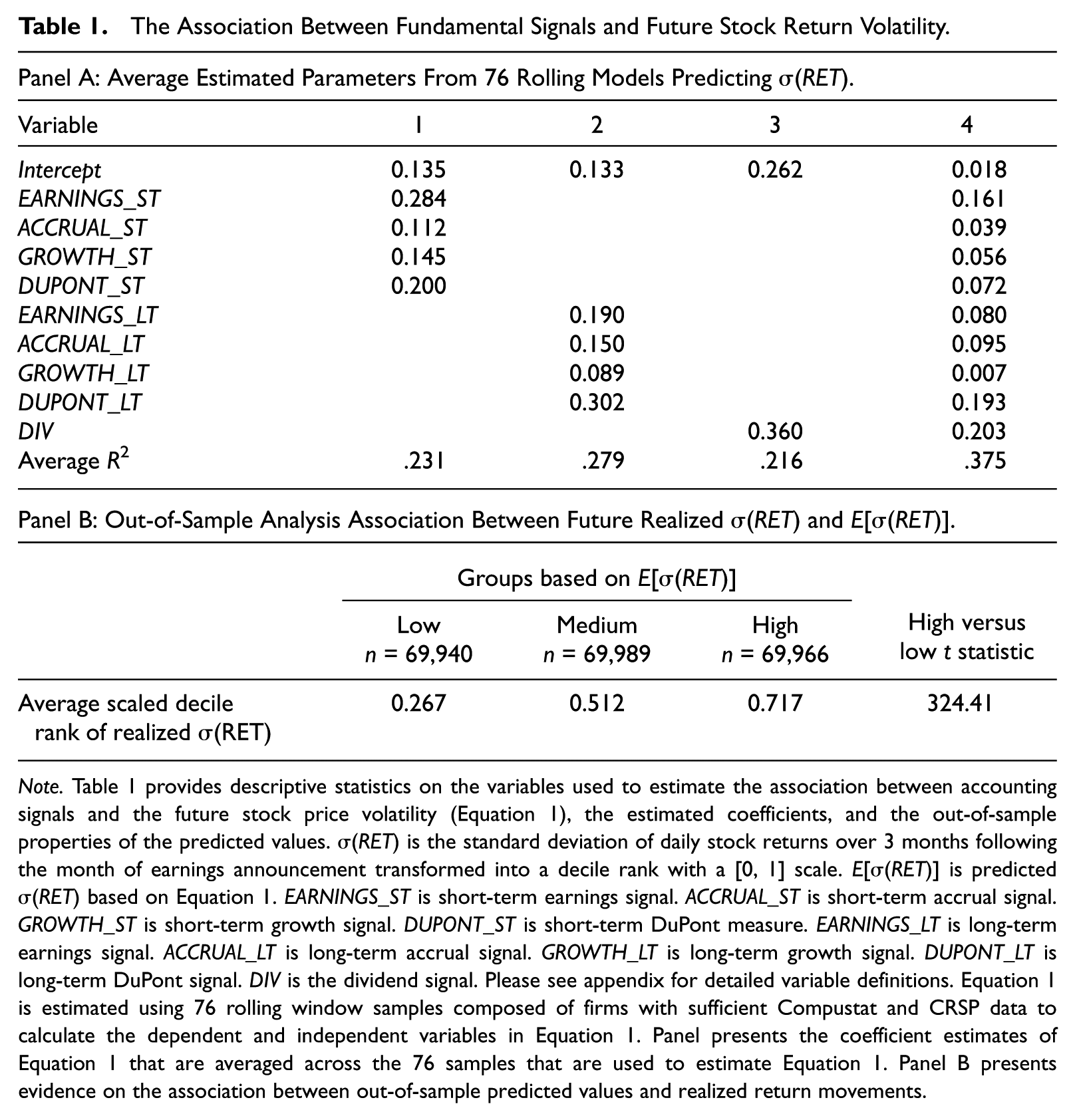
Note.Table 1 provides descriptive statistics on the variables used to estimate the association between accounting signals and the future stock price volatility (Equation 1), the estimated coefficients, and the out-of-sample properties of the predicted values. σ(RET) is the standard deviation of daily stock returns over 3 months following the month of earnings announcement transformed into a decile rank with a [0, 1] scale. E[σ(RET)] is predicted σ(RET) based on Equation 1. EARNINGS_ST is short-term earnings signal. ACCRUAL_ST is short-term accrual signal. GROWTH_ST is short-term growth signal. DUPONT_ST is short-term DuPont measure. EARNINGS_LT is long-term earnings signal. ACCRUAL_LT is long-term accrual signal. GROWTH_LT is long-term growth signal. DUPONT_LT is long-term DuPont signal. DIV is the dividend signal. Please see appendix for detailed variable definitions. Equation 1 is estimated using 76 rolling window samples composed of firms with sufficient Compustat and CRSP data to calculate the dependent and independent variables in Equation 1. Panel presents the coefficient estimates of Equation 1 that are averaged across the 76 samples that are used to estimate Equation 1. Panel B presents evidence on the association between out-of-sample predicted values and realized return movements.

Option Sample and Descriptive Statistics

Although the analysis of fundamental volatility in Table 1 is based on all firms with sufficient Compustat and CRSP (The Center for Research in Security Prices) data, we restrict the remainder of our analysis to the subset of those firms with sufficient Optionmetrics data to calculate straddle option returns (SRET_t₊₁). We calculate SRET_t₊₁ following Goyal and Saretto (2009). Specifically, we consider options that mature in the next month and select the contracts that are close to at-the-money, with moneyness between 0.975 and 1.025. To form a straddle, for each stock and for each month in the sample, we select the call and the put contracts with the same striking price that are close to at-the-month and expire the next month. After next-month expiration, we repeat the procedure and select a new pair of call and put contracts. As the straddle has both call and put contracts, the payoff to the straddle is determined purely by the deviation of stock price a month later from its exercise price. Whether the stock price goes up or down is irrelevant, a concept in line with the volatility channel that we emphasize in the article.

Matching our data on fundamental signals and historical volatility to Optionmetrics results in a sample of 98,723 firm-months composed of 58,060 firm-quarters (3,451 unique firms). A comparison of the number of firm-months with the number of firm-quarters reveals that we are typically able to use the information from a given firm-quarter for between one and two straddle positions (98,723/58,060= 1.700 monthly straddle contracts per firm-quarter) that are originated during the 3 months following the earnings announcement month.⁷

Ex ante, options investors may partially price the volatility information captured in fundamental signals. Therefore, E[σ(RET)] should be positively associated with implied volatility embedded in option contracts. To identify cases where the information from fundamental signals does not appear to be fully impounded into option prices, we adjust E[σ(RET)] relative to the level of implied volatility using the following model:

E [σ (RET)] = γ_{0} + γ_{1} IVO L_{t} + γ_{2} HVO L_{t} + e_{t},

where IVOL_t is the natural log of implied volatility from Optionmetrics in month t and HVOL_t is the natural log of the standard deviation of daily stock returns over the past year. By orthogonalizing our score based on fundamental signals against both IVOL_t and HVOL_t, we remove variation related to the Goyal and Saretto (2009) strategy, which is based on the difference between these two independent variables (DIFF_HVOL = HVOL – IVOL).

We label the residual from Equation 2 as DIFF_FUND, which is our main variable of interest to predict future option returns (Panel B of Figure 1 presents a timeline). A positive DIFF_FUND means fundamental volatility is high relative to implied volatility and historical volatility, suggesting both implied volatility and option prices are too low. Similarly, a negative DIFF_FUND means that fundamental volatility is low given the level of implied volatility and historical volatility, suggesting that options are too expensive.

Figure 1.

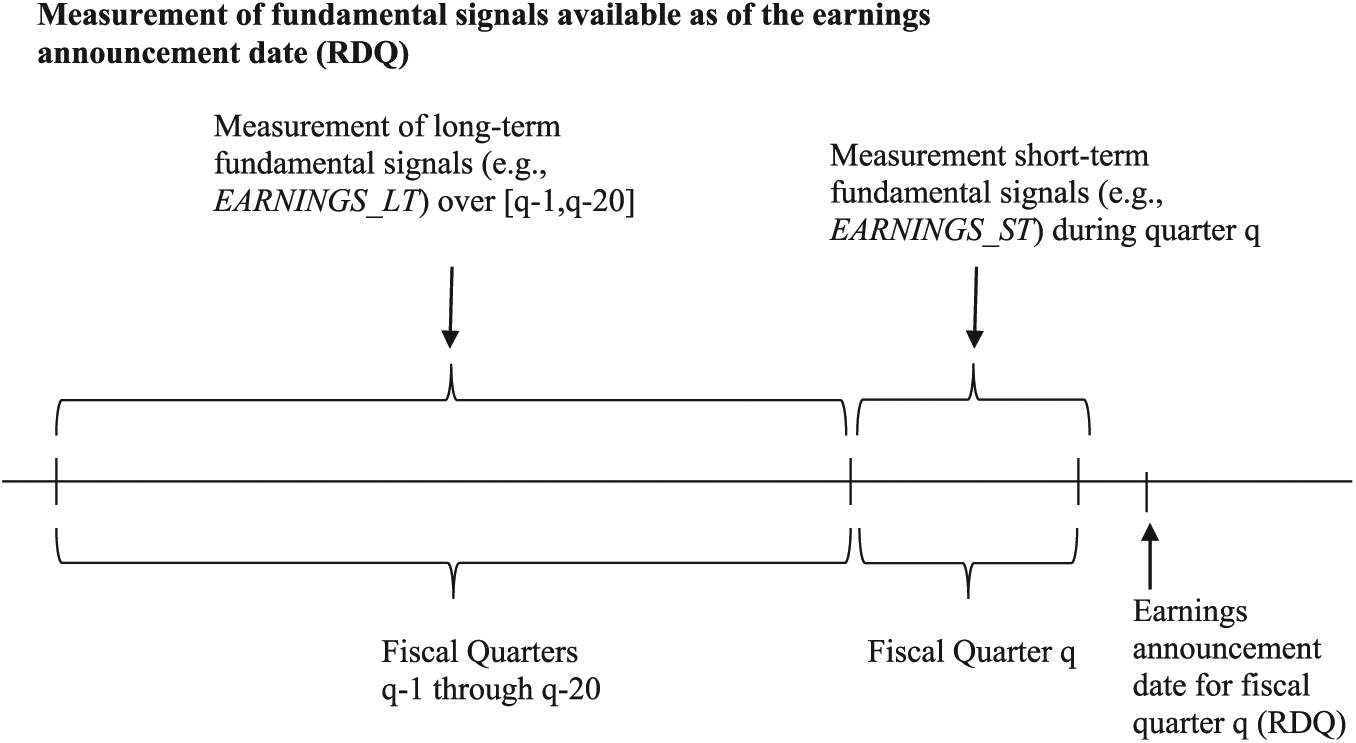
Timeline.

Panel A of Table 2 presents descriptive statistics for the monthly regression estimates of Equation 2. As expected, fundamental volatility proxied by E[σ(RET)] is positively correlated with implied volatility, suggesting that fundamental volatility is partially priced in the options market. In addition, there is a positive association with historical volatility, suggesting that fundamental volatility is one of the drivers of stock return volatility. However, the average monthly R² is 52.2%, indicating that cases exist in which E[σ(RET)] contains variation that is not explained by IVOL_t and HVOL_t.

Table 2.

Descriptive Statistics.

Panel A: Models to Estimate Abnormal Levels of E[σ(RET)]. $E [σ (RET)] = γ_{0} + γ_{1} IVO L_{t} + γ_{2} HVO L_{t} + error . (2)$
Independent variable	Coefficient (t statistic)
Intercept	0.760 (41.94)
IVOL_t	0.134 (3.69)
HVOL_t	0.228 (6.59)
R ²	.522

Panel B: Descriptive Statistics (N = 98,723).
Variable	M	SD	Q1	Median	Q3
SRET_t ₊₁	−0.008	0.827	−0.616	−0.185	0.397
IVOL_t	−1.035	0.446	−1.344	−1.039	−0.734
HVOL_t	−1.009	0.453	−1.333	−1.017	−0.703
DIFF_FUND	0.000	0.124	−0.087	−0.003	0.083

Panel C: Correlation Matrix (Pearson Upper Triangle, Spearman Lower Triangle).
Variable	(1)	(2)	(3)	(4)
(1) SRET_t₊₁	1.000	−0.014	−0.008	0.032
(2) IVOL	−0.016	1.000	0.845	0.000
(3) HVOL	−0.009	0.844	1.000	0.000
(4) DIFF_FUND	0.024	0.030	0.028	1.000

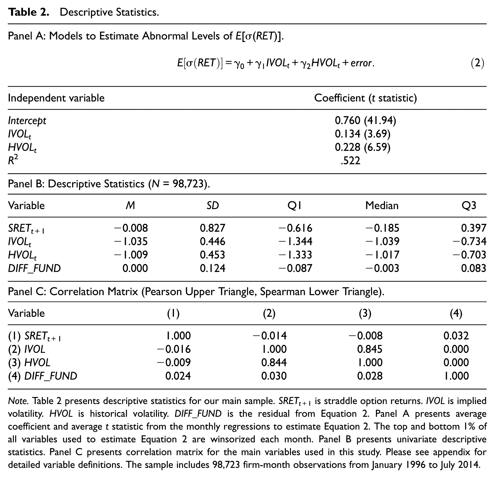
Note.Table 2 presents descriptive statistics for our main sample. SRET_t₊₁ is straddle option returns. IVOL is implied volatility. HVOL is historical volatility. DIFF_FUND is the residual from Equation 2. Panel A presents average coefficient and average t statistic from the monthly regressions to estimate Equation 2. The top and bottom 1% of all variables used to estimate Equation 2 are winsorized each month. Panel B presents univariate descriptive statistics. Panel C presents correlation matrix for the main variables used in this study. Please see appendix for detailed variable definitions. The sample includes 98,723 firm-month observations from January 1996 to July 2014.

Panel B of Table 2 presents descriptive statistics for firm-months with both fundamental signal and straddle return data. The mean (median) SRET_t₊₁ is −0.008 (−0.185), a result consistent with the prior literature and suggesting that straddle contracts on average lose money. Panel C of Table 2 reports the correlation matrix of the main variables of interest in this study. We observe that DIFF_FUND has a positive association with straddle option returns (SRET_t₊₁), consistent with the main empirical prediction of the article. As expected, IVOL and HVOL exhibit a strong positive correlation, suggesting that while implied volatility may not efficiently capture all the information in historical volatility, these two signals overlap considerably. Given that DIFF_FUND is the residual from Equation 2, the Pearson correlation between DIFF_FUND and IVOL and HVOL is 0.

Empirical Evidence

Main Results on Fundamental Signals and Future Option Returns

In this section, we use both portfolio and regression approaches to formally investigate whether accounting information predicts future option returns. Under the portfolio approach, for each month, we sort straddle options into 10 deciles based on the variable of interest. For comparison purposes, we first replicate Goyal and Saretto’s (2009) historical volatility strategy in our sample. In Table 3, column 1 of Panel A shows that option returns increase from −10.6% in D1 to 7.7% in D10, resulting in a D10 – D1 hedge return of 18.3% (t = 9.79) per month.

Table 3.

Fundamental Score and Future Option Returns.

Panel A: Portfolio Analysis.
Deciles	Replication of Goyal and Saretto (2009) in our sample (DIFF_HVOL)	Option returns of portfolios based on fundamental signals (DIFF_FUND)	Stock returns of portfolios based on fundamental signals (DIFF_FUND)
D1	−0.106	−0.066	0.012
D2	−0.041	−0.033	0.011
D3	−0.048	−0.026	0.011
D4	−0.021	−0.032	0.010
D5	−0.021	−0.005	0.012
D6	0.008	−0.012	0.011
D7	−0.002	−0.007	0.012
D8	0.007	0.030	0.012
D9	0.036	0.011	0.014
D10	0.077	0.028	0.015
HEDGE	0.183	0.094	0.003
(D10 – D1)	(9.79)	(7.60)	(1.33)
Panel B: Fama–MacBeth Regressions of Future Straddle Option Returns.
Independent variables	1	2	3
Intercept	−0.052 (−3.00)	−0.080 (−5.56)	−0.122 (−7.57)
DIFF_FUND	0.082 (8.10)		0.083 (8.18)
DIFF_HVOL		0.139 (9.51)	0.140 (9.55)
R ²	.005	.009	.014

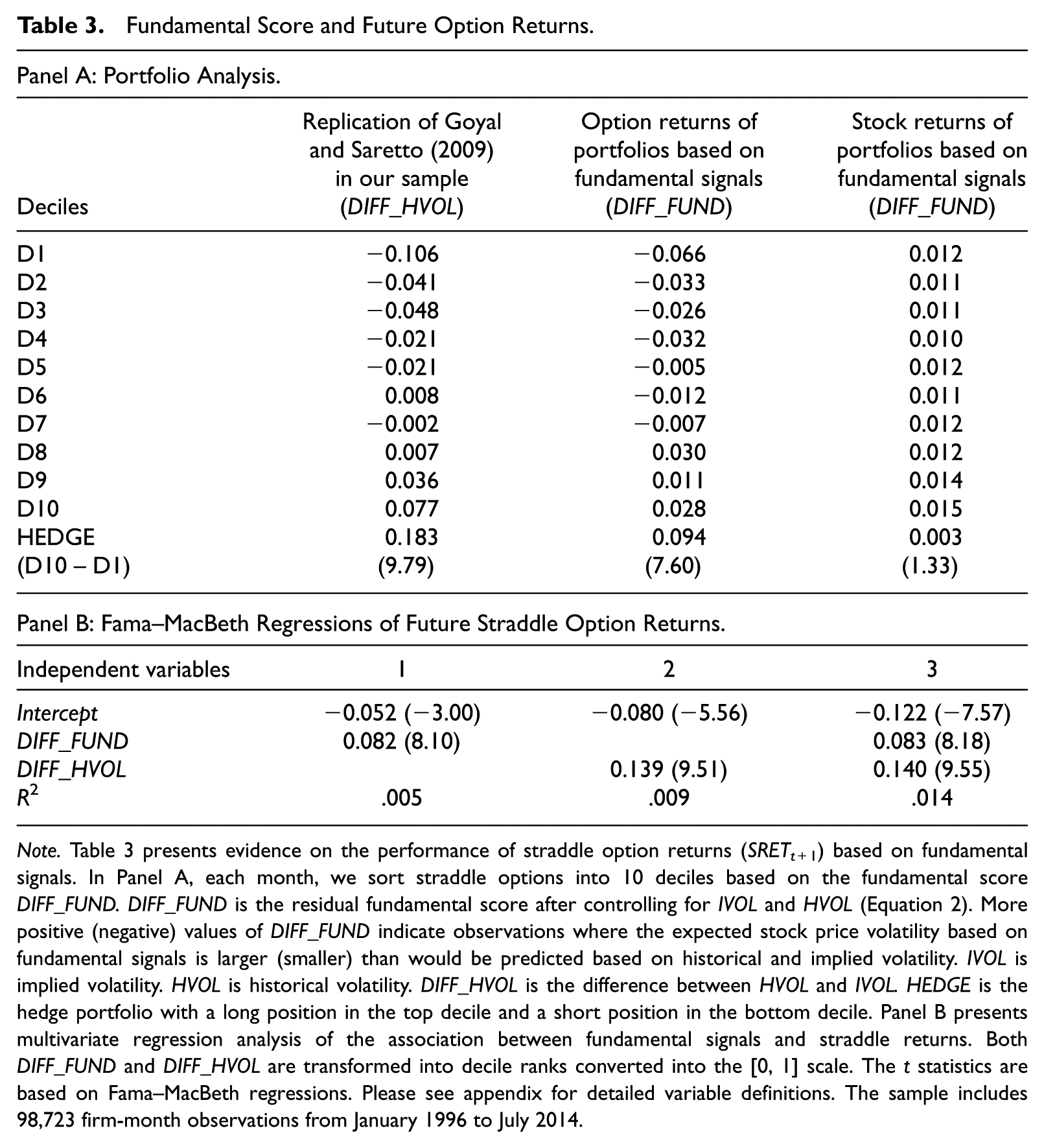
Note.Table 3 presents evidence on the performance of straddle option returns (SRET_t₊₁) based on fundamental signals. In Panel A, each month, we sort straddle options into 10 deciles based on the fundamental score DIFF_FUND. DIFF_FUND is the residual fundamental score after controlling for IVOL and HVOL (Equation 2). More positive (negative) values of DIFF_FUND indicate observations where the expected stock price volatility based on fundamental signals is larger (smaller) than would be predicted based on historical and implied volatility. IVOL is implied volatility. HVOL is historical volatility. DIFF_HVOL is the difference between HVOL and IVOL. HEDGE is the hedge portfolio with a long position in the top decile and a short position in the bottom decile. Panel B presents multivariate regression analysis of the association between fundamental signals and straddle returns. Both DIFF_FUND and DIFF_HVOL are transformed into decile ranks converted into the [0, 1] scale. The t statistics are based on Fama–MacBeth regressions. Please see appendix for detailed variable definitions. The sample includes 98,723 firm-month observations from January 1996 to July 2014.

Column 2 shows a positive association between DIFF_FUND and decile option returns. Straddle option returns increase fairly monotonically from −6.6% in D1 to 2.8% in D10, resulting in a D10 – D1 hedge return of 9.4% per month (t = 7.60). This evidence suggests that fundamental volatility is positively associated with future straddle returns, consistent with option investors underweighting accounting information.

We also examine stock returns of 10 DIFF_FUND portfolios to ensure that our variable captures the volatility channel rather than the cash flow channel. We measure stock returns in the same window as we measure option returns from the portfolio formation date to option expiration date. Column 3 of Panel A shows that future stock returns are largely similar across 10 DIFF_FUND deciles. The D10 – D1 hedge portfolio using stock returns is not significantly different from 0 at conventional levels (t = 1.33). Similar stock returns across DIFF_FUND deciles support the thesis of the article that our fundamental variables capture the volatility information rather than any information about future cash flows.

Finally, we use a multivariate regression framework to supplement our portfolio results. Specifically, we consider the following regression model:

SRE T_{t + 1} = α_{0} + α_{1} DIFF_FUN D_{t} + α_{2} DIFF_HVO L_{t} + e_{t + 1},

where the explanatory variables are transformed into decile rankings on a [0, 1] scale.

Panel B of Table 3 presents the regression results. Column 1 (column 2) contains a univariate model where only DIFF_FUND (DIFF_HVOL) is included as an independent variable. We find positive and significant coefficients on DIFF_FUND and DIFF_HVOL, a result consistent with the portfolio results in Panel A. In column 3, we include both measures in the model and find that both coefficients are highly significant, providing further evidence that fundamental signals convey incremental information with respect to future straddle returns.

Is a Fundamental-Based Option Strategy Risky?

To assess whether our fundamental-based option strategy is risky, we conduct two sets of analysis. First, we examine the comovement between hedge portfolio returns and common risk factors. The finance literature suggests that theoretical asset pricing models, such as CAPM (capital asset pricing model), also apply to options (e.g., Coval & Shumway, 2001). The intuition is that common state variables, such as consumption, capture all kinds of risks in the capital markets, including the options market. Therefore, the expected return on an option should relate to the option’s sensitivity to common risk factors. Empirically, prior studies use common return factors to capture systematic risks (e.g., Boyer & Vorkink, 2011; Choy, 2011; Goyal & Saretto, 2009). Following prior work, we use the four-factor model below to examine whether our fundamental trading strategy exposes investors to systematic risks.⁸

SRE T_{HEDGE} = α + β_{1} MK T_{RF} + β_{2} SMB + β_{3} HML + β_{4} MOM + e,

where SRET_HEDGE is the D10 – D1 hedge portfolio return based on DIFF_FUND. MKT_RF, SMB, HML, and MOM are the market, size, book-to-market, and momentum factors, respectively. The four-factor data are from Kenneth French’s website. The intercept ( $α$ ) provides an estimate of the monthly abnormal returns earned by the DIFF_FUND trading strategy after controlling for these four factors. As our straddle contracts typically span 2 months (e.g., a straddle initiated on May 19 that expires on June 21) and do not all start on the same date, we present results for two versions of Equation 4 using the factors for the initiation and the expiration months.

Panel A of Table 4 presents the analysis of the hedge return from the DIFF_FUND trading strategy. In Models 1 and 2, abnormal returns (intercepts) and their associated t statistics from the four-factor model are virtually the same as the raw returns reported in Panel A of Table 3. In addition, while the coefficients on the HML factor are negative and significant, the coefficients on the other factors are insignificant regardless of whether the factors for the initiation or the expiration months are considered. In sum, the results suggest that the hedge portfolio returns from our option strategies are not explained by the four common factors.

Table 4.

Evaluation of Monthly Returns From Fundamental Analysis Portfolios.

Panel A: Four-Factor Model on the Hedge Portfolio Returns Based on DIFF_FUND.
	Risk data in month t	Risk data in month t+ 1
Intercept	0.097 (7.66)	0.099 (7.85)
MKT_RF	−0.082 (−0.27)	−0.345 (−1.17)
SMB	−0.428 (−1.12)	−0.075 (0.20)
HML	−0.721 (−1.77)	−0.980 (−2.42)
UMD	0.029 (0.12)	−0.060 (−0.25)
R ²	.017	.030

Panel B: Distribution of the D10 – D1 Hedge Returns Based on DIFF_FUND.	Percent
Percent of months with returns less than 0%	0.278
Percent of months with returns less than −10%	0.139
Percent of months with returns less than −20%	0.067
Percent of months with returns less than −30%	0.031
Percent of months with returns less than −40%	0.004
Percent of months with returns less than −50%	0.000

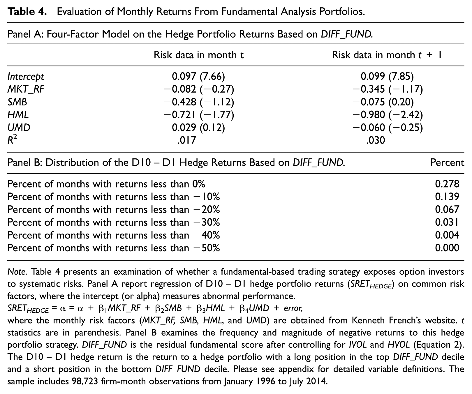
Note.Table 4 presents an examination of whether a fundamental-based trading strategy exposes option investors to systematic risks. Panel A report regression of D10 – D1 hedge portfolio returns (SRET_HEDGE) on common risk factors, where the intercept (or alpha) measures abnormal performance.

SRET_HEDGE = α = α+β₁MKT_RF+β₂SMB+β₃HML+β₄UMD+error,

where the monthly risk factors (MKT_RF, SMB, HML, and UMD) are obtained from Kenneth French’s website. t statistics are in parenthesis. Panel B examines the frequency and magnitude of negative returns to this hedge portfolio strategy. DIFF_FUND is the residual fundamental score after controlling for IVOL and HVOL (Equation 2). The D10 – D1 hedge return is the return to a hedge portfolio with a long position in the top DIFF_FUND decile and a short position in the bottom DIFF_FUND decile. Please see appendix for detailed variable definitions. The sample includes 98,723 firm-month observations from January 1996 to July 2014.

Our second set of analyses examines the time-series properties of our fundamental analysis portfolio. An alternative risk-based perspective suggests that portfolios with higher average returns must have inconsistent performance. Investors may have positive returns over a long window, but the portfolio strategy exposes the investor to large negative outcomes. This concern particularly arises for options-based trading strategies, where selling a straddle exposes the seller to potentially extreme negative outcomes. To address this concern, we examine the performance of our fundamental analysis portfolio over time, noting the overall frequency of negative returns and the performance by year.

Panel B of Table 4 provides further details on the distribution of monthly returns for the D10 – D1 hedge return. The fundamental strategy delivers positive returns for 70% of months during the sample window. The hedge returns are less than –20% for less than 7% of months in the sample period. Finally, Figure 2 plots the average monthly hedge returns by year. The average monthly hedge return is positive for all the 19 years in the sample period.

Figure 2.

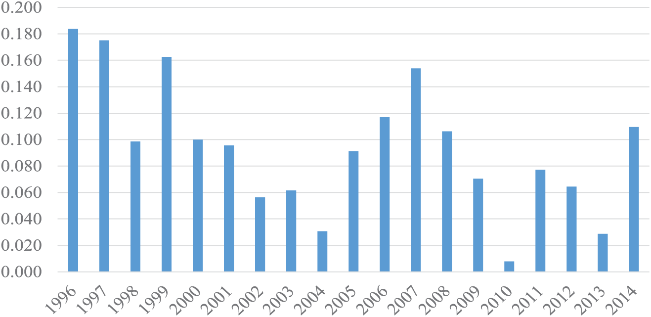
Average monthly returns to fundamental-based hedge portfolios over time.

In summary, we find fairly consistent strong positive returns for the fundamental-based option strategy. Our evidence is unlikely to reflect an appropriate reward for a risky investment strategy caused by the long positions being more risky than the short positions in the strategy.

Combing Fundamental and Historical Volatility Signals

In this section, we consider how investors could combine fundamental signals and historical volatility together in their trading strategies. As the previous sections show that fundamental signals contain information about future straddle returns that is incremental to what is captured in historical volatility, we expect higher hedge returns by combining historical volatility with fundamental signals.

We begin with the bottom and top deciles (D1 and D10) of DIFF_HVOL, which are the short and long positions in Goyal and Saretto (2009). Next, we further sort the observations in the D1 and D10 into four quartiles, each based on DIFF_FUND. Average straddle returns for each of these groups are reported in Panel A of Table 5. Below we discuss an approach to combine these signals.

Table 5.

Combining Fundamental Signals and Historical Volatility Into a Single Trading Strategy.

Panel A: Combine Fundamental Score With Historical Volatility Signals.
	DIFF_FUND
	Q1	Q2	Q3	Q4
D1(DIFF_HVOL)	−0.159	−0.108	−0.098	−0.058
D10(DIFF_HVOL)	0.037	0.065	0.098	0.107
Panel B: Hedge Returns.
	Short position	Long position	Hedge (long-short)	Hedget statistic
AGREE	−0.159	0.107	0.266	9.61
DISAGREE	−0.089	0.067	0.156	7.95
Difference AGREE – DISAGREE			0.110 (4.15)

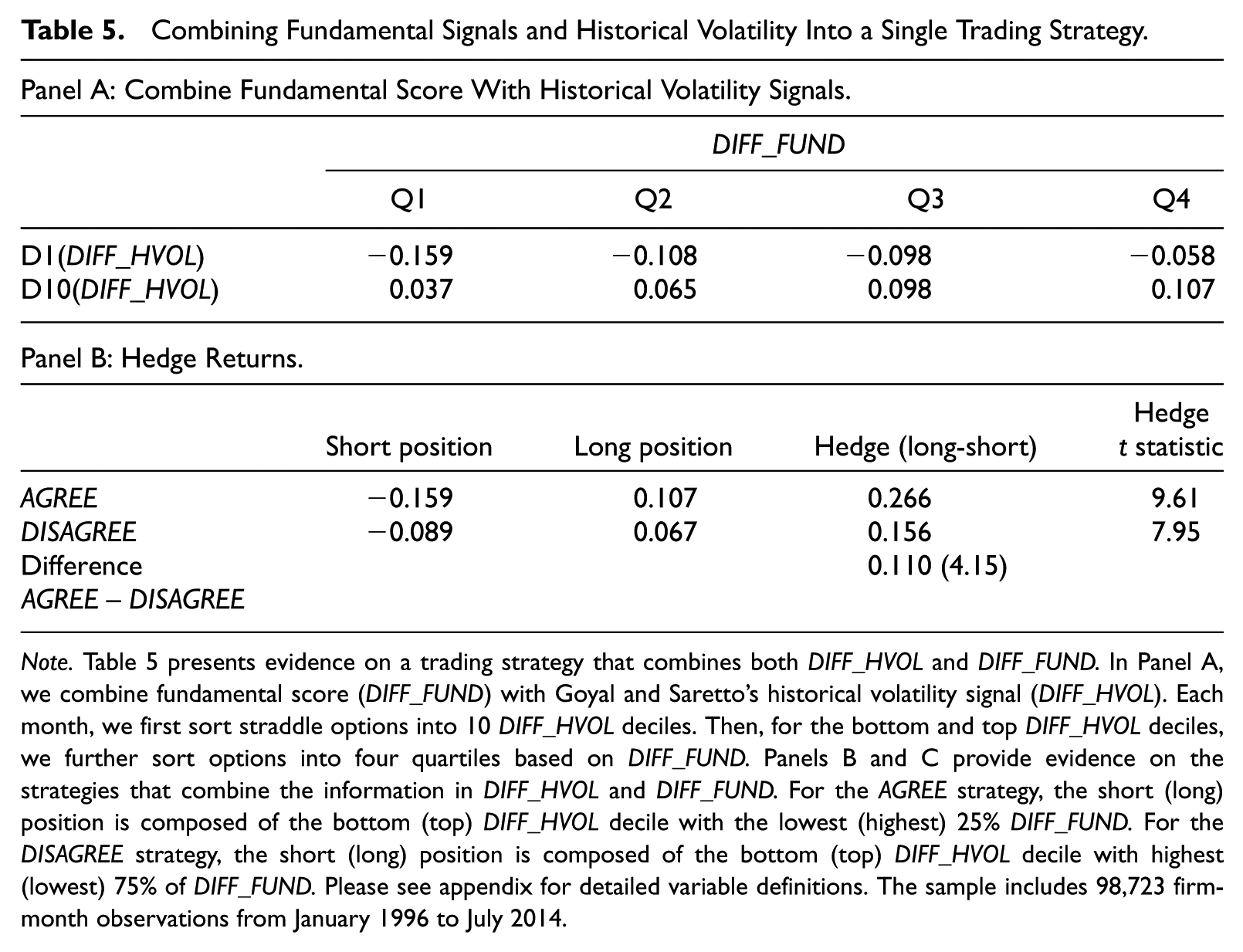
Note.Table 5 presents evidence on a trading strategy that combines both DIFF_HVOL and DIFF_FUND. In Panel A, we combine fundamental score (DIFF_FUND) with Goyal and Saretto’s historical volatility signal (DIFF_HVOL). Each month, we first sort straddle options into 10 DIFF_HVOL deciles. Then, for the bottom and top DIFF_HVOL deciles, we further sort options into four quartiles based on DIFF_FUND. Panels B and C provide evidence on the strategies that combine the information in DIFF_HVOL and DIFF_FUND. For the AGREE strategy, the short (long) position is composed of the bottom (top) DIFF_HVOL decile with the lowest (highest) 25% DIFF_FUND. For the DISAGREE strategy, the short (long) position is composed of the bottom (top) DIFF_HVOL decile with highest (lowest) 75% of DIFF_FUND. Please see appendix for detailed variable definitions. The sample includes 98,723 firm-month observations from January 1996 to July 2014.

First, we identify cases where the fundamental and historical volatility signals agree; we label this strategy AGREE. We pick options in D1 with the bottom quartile of fundamental score as our short position and options in D10 with the top quartile of fundamental score as our long position. Panel B of Table 5 provides an analysis of the returns to combining these two types of signals. Consistent with our expectations, incorporating fundamental signals into the historical volatility strategy increases the hedge return from 18.3% in Panel A of Table 3 to 26.6% in Panel B of Table 5.

To contrast with the AGREE strategy, we also calculate the hedge returns when the two sets of signals disagree (DISAGREE). This hedge portfolio is defined as a long position in D10(DIFF_HVOL) for firms where DIFF_FUND is not in the top quartile and a short position in D1(DIFF_HVOL) for firms where DIFF_FUND is not in the bottom quartile. This strategy yields much lower returns (15.6%). Furthermore, Panel A presents a test of the difference in returns between these two strategies, which is positive and significant (difference = 11.0%, t = 4.15), providing evidence that the fundamental volatility plays a significant role in the mispricing documented by Goyal and Saretto (2009). We also present the average monthly returns by year from the AGREE and DISAGREE strategies in Figure 3. The average monthly returns from the AGREE strategy exceed those from the DISAGREE strategy in 15 of the 19 years.

Figure 3.

Average monthly returns to combined strategy hedge portfolios over time.Note. Figure 3 presents the returns to the AGREE and DISAGREE combined strategies. For the AGREE strategy, the short (long) position is composed of the bottom (top) DIFF_HVOL decile with the lowest (highest) 25% DIFF_FUND. For the DISAGREE strategy, the short (long) position is composed of the bottom (top) DIFF_HVOL decile with highest (lowest) 75% of DIFF_FUND.

In sum, historical volatility and fundamental signals are complements and the two signals can be combined. This suggests that similar to the use of fundamental analysis to enhance the value strategy (Piotroski, 2000), fundamental analysis related to fundamental volatility can enhance option-based trading strategies.

The Impact of Transaction Costs

In this section, we examine the impact of transaction costs on trading strategy performance. Specifically, we consider the impact of the bid–ask spread, which is crucial in interpreting empirical results in option studies.⁹ The bid–ask spread is typically much higher in the option market than in the stock market. The main results in previous sections are based on the assumption that options are traded at the midpoint of bid and ask prices. It is possible that investors cannot trade options at that price in every circumstance. Many finance studies (e.g., De Fontnouvelle, Fisher, & Harris, 2003; Maydew, 2002) show that the effective spreads for options are large in absolute terms but are typically much smaller than the quoted spreads, with the effective to quoted spread ratio to be less than 0.50. To examine the impact of transaction costs, we recalculate option returns under the assumption that the effective spread is equal to the quoted spread (the effective-to-quoted spread ratio of 1): investors always buy options at the ask price and write options at the bid price. We view this assumption as conservative because it produces the lowest after transaction cost returns relative to alternative effective spread assumptions used by prior literature. As tick-by-tick option transaction data are not available, we follow the prior literature and use the closing bid–ask spread to proxy for the average bid–ask spread.

We repeat the main analysis using option returns after transaction costs and report empirical results in Table 6. The hedge return from historical volatility strategy drops from 18.3% (t = 9.79) to −4.8% (t = −2.22).¹⁰ We find that the D10 – D1 hedge return from fundamental volatility DIFF_FUND drops from 9.4% (t = 7.60) before transaction costs to −9.0% (t = −5.94) after transaction costs. The inability of the returns for the fundamental or historical volatility strategy in isolation to exceed transaction costs provides evidence consistent with a “limits to arbitrage” framework (Shleifer & Vishny, 1997). The returns tests suggest that option prices do not fully capture fundamental or historical volatility signals. However, transaction costs are sufficiently large to limit an arbitrageur’s ability to profit from option mispricing in isolation, allowing the mispricing to exist.

Table 6.

The Analysis of Transaction Costs.

Hedge Portfolio (D10 – D1) Return Before Versus After Transaction Costs.
Hedge return based on	Before transaction costs	After transaction costs
DIFF_HVOL	0.183 (9.79)	−0.048 (−2.22)
DIFF_FUND	0.094 (7.60)	−0.090 (−5.94)
AGREE	0.266 (9.61)	0.039 (1.32)
DISAGREE	0.156 (7.95)	−0.075 (−3.21)

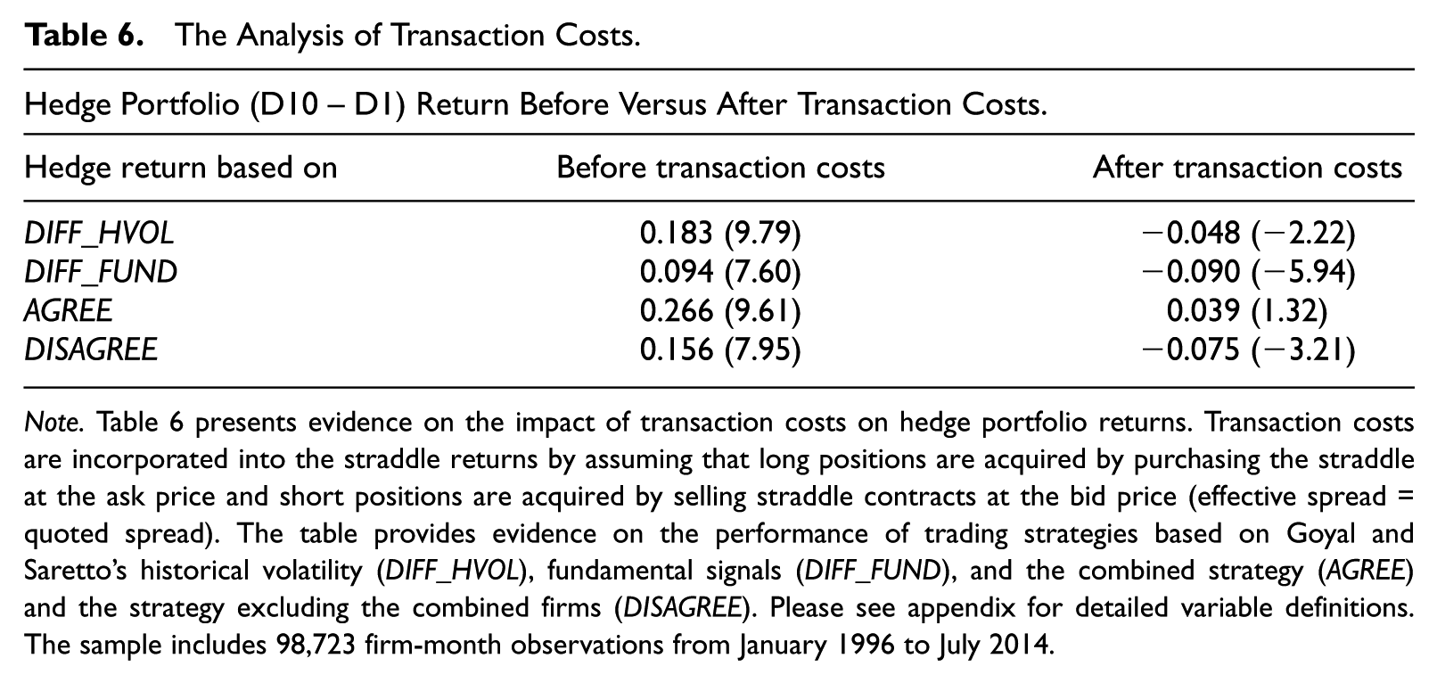
Note.Table 6 presents evidence on the impact of transaction costs on hedge portfolio returns. Transaction costs are incorporated into the straddle returns by assuming that long positions are acquired by purchasing the straddle at the ask price and short positions are acquired by selling straddle contracts at the bid price (effective spread = quoted spread). The table provides evidence on the performance of trading strategies based on Goyal and Saretto’s historical volatility (DIFF_HVOL), fundamental signals (DIFF_FUND), and the combined strategy (AGREE) and the strategy excluding the combined firms (DISAGREE). Please see appendix for detailed variable definitions. The sample includes 98,723 firm-month observations from January 1996 to July 2014.

We also explore the effect of transaction costs on the returns from our combined strategies. The AGREE return drops from 26.6% to 3.9%. Although positive, the posttransaction cost returns are not significant at conventional levels (t = 1.32). For comparison, the DISAGREE strategy has posttransaction costs returns that are negative (−7.5%, t = −3.21). As in Table 5, the difference between the AGREE and DISAGREE strategy returns is positive and significant (t = 3.78, not tabulated), suggesting that the DIFF_HVOL strategy performs significantly better using after transaction cost returns among the sample of firms where fundamental volatility signals reinforce the DIFF_HVOL signal.

Our second approach to address the transaction cost issue is to examine cross-sectional variations in trading strategy performance based on the proxies for transaction costs and liquidity. Specifically, we consider three proxies: firm size, the bid–ask spread, and option trading volume. For each proxy, we partition our sample into high (above median) and low (below median) groups each month and then implement our combined trading strategies (AGREE and DISAGREE) within each resulting group. To offset the reduction in sample from the high/low partition, we slightly revise the definition of AGREE and DISAGREE. Specifically, For the AGREE strategy, the short (long) position is composed of the bottom (top) DIFF_HVOL decile with the lowest (highest) 50% DIFF_FUND. For the DISAGREE strategy, the short (long) position is composed of the bottom (top) DIFF_HVOL decile with highest (lowest) 50% of DIFF_FUND. Using the median, rather than a quartile in these definitions, allows us to include twice as many firms in the AGREE strategy, which is valuable given that the high/low partition reduces the sample size in half. The results are reported in Panels A, B, and C of Table 7.

Table 7.

The Analysis of Transaction Costs Across Subsamples.

Panel A: Hedge Portfolio Returns Partitioned Based on Firm Size.
Hedge return based on	Before transaction costs		After transaction costs
Hedge return based on	Bottom size group	Top size group	Bottom size group	Top size group
AGREE	0.303 (10.03)	0.214 (7.40)	−0.056 (−1.24)	0.094 (3.35)
DISAGREE	0.175 (5.96)	0.062 (2.26)	−0.108 (−3.51)	−0.058 (−2.12)
Difference	0.129 (3.53)	0.152 (4.25)	0.052 (1.08)	0.152 (4.23)
Panel B: Hedge Portfolio Returns Partitioned Based on Bid–Ask Spread.
Hedge return based on	Before transaction costs		After transaction costs
Hedge return based on	Bottom spread group	Top spread group	Bottom spread group	Top spread group
AGREE	0.181 (5.95)	0.290 (9.05)	0.106 (3.59)	−0.122 (−2.57)
DISAGREE	0.079 (2.88)	0.144 (5.34)	0.001 (0.05)	−0.172 (−5.58)
Difference	0.102 (2.93)	0.146 (3.93)	0.105 (3.01)	0.050 (0.98)
Panel C: Hedge Portfolio Returns Partitioned Based on Option Trading Volume.
Hedge return based on	Before transaction costs		After transaction costs
Hedge return based on	Bottom volume group	Top volume group	Bottom volume group	Top volume group
AGREE	0.227 (8.56)	0.213 (7.09)	−0.143 (−3.51)	0.103 (3.57)
DISAGREE	0.143 (5.00)	0.097 (3.53)	−0.188 (−4.77)	−0.008 (0.29)
Difference	0.084 (2.40)	0.116 (3.41)	0.044 (0.93)	0.111 (3.29)

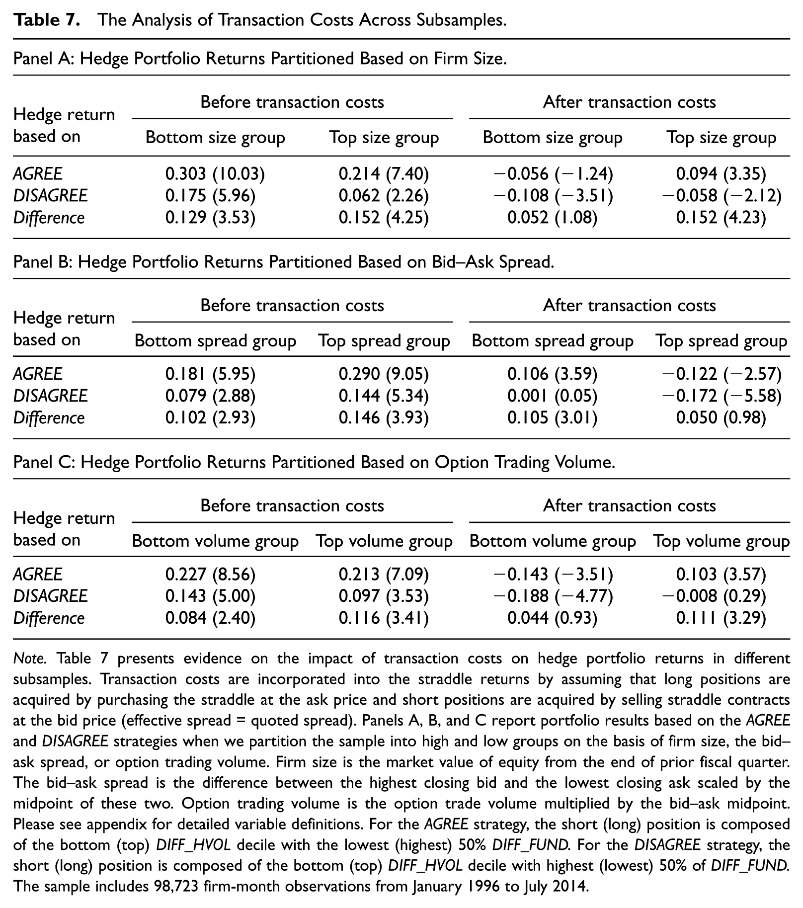
Note.Table 7 presents evidence on the impact of transaction costs on hedge portfolio returns in different subsamples. Transaction costs are incorporated into the straddle returns by assuming that long positions are acquired by purchasing the straddle at the ask price and short positions are acquired by selling straddle contracts at the bid price (effective spread = quoted spread). Panels A, B, and C report portfolio results based on the AGREE and DISAGREE strategies when we partition the sample into high and low groups on the basis of firm size, the bid–ask spread, or option trading volume. Firm size is the market value of equity from the end of prior fiscal quarter. The bid–ask spread is the difference between the highest closing bid and the lowest closing ask scaled by the midpoint of these two. Option trading volume is the option trade volume multiplied by the bid–ask midpoint. Please see appendix for detailed variable definitions. For the AGREE strategy, the short (long) position is composed of the bottom (top) DIFF_HVOL decile with the lowest (highest) 50% DIFF_FUND. For the DISAGREE strategy, the short (long) position is composed of the bottom (top) DIFF_HVOL decile with highest (lowest) 50% of DIFF_FUND. The sample includes 98,723 firm-month observations from January 1996 to July 2014.

Panel A of Table 7 indicates that the before transaction cost hedge returns from the AGREE strategy are greater than those from the DISAGREE strategy for both the low- and high-size groups (t = 3.53 and 4.25). In addition, the after transaction cost returns from the AGREE strategy are significantly positive for the large firm group (t = 3.35), while the returns to the DISAGREE are negative and significant (t = −2.12).

In Panels B and C, we continue to find that the after transaction costs hedge returns from the AGREE strategy are positive and significant for subsamples of options with low transaction costs: for options with low bid–ask spreads (t = 3.59) and for options with large trading volume (t = 3.57).

In sum, we find that transaction costs significantly affect the performance of the trading strategy based on fundamental volatility or historical volatility in isolation. For the overall sample, the D10 – D1 hedge returns drop from a significantly positive level before transaction costs to a negative level after transaction costs. However, the combination of fundamental signals with historical volatility can produce a trading strategy that yields significantly positive hedge returns for options with low transaction costs.

Additional Analyses and Sensitivity Checks

The Time-Series Pattern of Implied Volatility around the Portfolio Formation Date

We have motivated our analysis from the fundamental volatility perspective. That is, our fundamental signals capture fundamental volatility, and implied volatility may deviate from the true underlying volatility. In portfolios sorted by our fundamental score, implied volatility is too low relative to fundamental volatility for D10 options and too high for D1 options. If this story holds, a natural prediction is that implied volatility should increase for D10 options and decline for D1 options after the portfolio formation date, given that over time, implied volatility should converge to the true underlying volatility.

In Figure 4, we plot the time-series pattern of implied volatility of D1 and D10 options based on DIFF_FUND. We consider a range of 12 months before and 12 months after the portfolio formation date (t = 0). The results are striking. For D1 options, implied volatility is higher at Time 0 than in previous months. After Time 0, implied volatility decreases to the level of the previous months. In contrast, for D10 options, implied volatility is much lower at Time 0 than in adjacent months, resulting in a clean “V” shape of implied volatility. Overall, the results are consistent with the story that implied volatility temporally deviates from fundamental volatility, resulting in predictable option returns.

Figure 4.

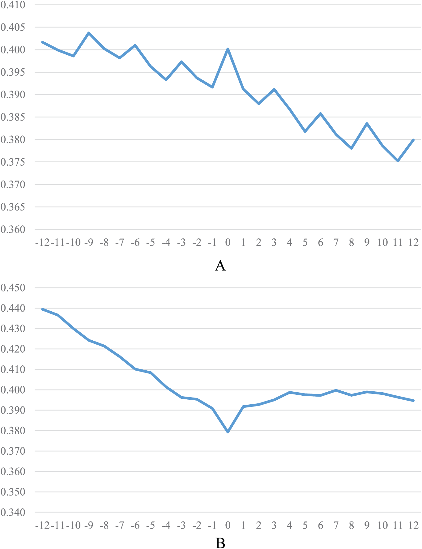
The time-series pattern of implied volatility around the portfolio formation date.

The Analysis of Individual Fundamental Signals

In the main analysis, we aggregate individual fundamental signals into a single score when examining future option returns. To complement this analysis, we transform each signal into a decile rank and include those signals as well as HVOL and IVOL in a regression predicting future straddle returns. The coefficients on the individual fundamental signals (untabulated) suggest a degree of inefficiency with respect to both short-term and long-term fundamental signals. In addition, when estimating the regression, we also examine the sum of the coefficients that can also be interpreted as the hedge portfolio returns based on individual fundamental signals (Abarbanell & Bushee, 1998). To provide further insight into the pricing of short-term and long-term signals, we estimate a model that includes only the short-term fundamental signals and a model that includes only the long-term fundamental signals. In each of these specifications, the sum of the coefficients on the fundamental signals is highly significant. These findings are consistent with both the evidence in Goyal and Saretto (2009) that option prices underreact to long-term signals and the literature on drift in accounting suggesting that prices underreact to short-term accounting signals.

A Simplified Strategy to Mitigate Data Mining Concerns

Our set of fundamental signals is an expanded version of Beneish et al. (2001). To avoid the risk of data mining, we repeat our analysis based on eight fundamental signals identified in Beneish et al. (2001): sales growth, sales growth decline indicator, changes in earnings, loss indicator, R&D intensity, accruals, capital expenditures, and changes in gross margins.¹¹ We observe a noticeably smaller R² (8.2% vs. 37.5% in Table 1), suggesting that excluding some signals from our main analysis could limit the power of these tests.

We repeat the analysis from Tables 3 and 5 using these signals. We continue to observe a smaller but positive and significant association between straddle returns and the fundamental signals, using the hedge return test or the multivariate regression test (Equation 3). This evidence suggests that even a limited set of accounting signals can predict option returns. In addition, we continue to observe that there are benefits from combining signals (i.e., the returns to the AGREE strategy are significantly greater than the returns to the DISAGREE strategy).

Other Robustness Checks

To complement our analysis using the Black–Scholes model implied volatility provided by Optionmetrics; we also consider an alternative implied volatility measure, model-free implied volatility. Following the technique described in Sridharan (2015), we estimate implied volatility based on the prices of put and call options from the Optionmetrics volatility surface data set.¹² We repeat our main analysis using this alternative volatility measure. We continue to observe support for our article’s central prediction that accounting information provides additional information about future option returns.

In another contemporaneous article, Sridharan (2015) examines the association between fundamental signals and straddle returns. Sridharan (2015) uses an accounting-based asset pricing model (Penman, Reggiani, Richardson, & Tuna, 2015) to link the volatility of returns to the volatility of earnings yields and the volatility of changes in the market-to-book premium. To explore the overlap between her signals, we calculate the natural log of the standard deviation of earnings yields and the natural log of the standard deviation of changes in market-to-book premiums over the window we use to calculate our long window signals.¹³ We continue to observe that our fundamental signals have a positive and significant association with future straddle returns after controlling for the variables in Sridharan (2015).

Conclusion

In this article, we examine the extent to which accounting information is useful in evaluating the volatility of a firm’s operations and whether this information is appropriately priced by the options market. We find evidence that information about a firm’s fundamental volatility is not fully priced in option contracts. Hedge portfolios with long and short straddle contract positions based on accounting signals earn statistically and economically significant returns before transaction costs. However, the high level of transaction costs in the options market limits the profitability of fundamental trading strategy in isolation. We also show that a strategy that combining fundamental signals with historical volatility can produce significantly positive hedge returns after transaction costs in cases where transaction costs are low.

Overall, our evidence provides insight into a new dimension of fundamental analysis—using accounting signals to evaluate fundamental volatility and examining whether such information is priced in the options market. Our evidence complements prior fundamental analysis research on equity returns, which focused on fundamental signals to predict future operating performance and stock returns.

Footnotes

Appendix

Appendix.

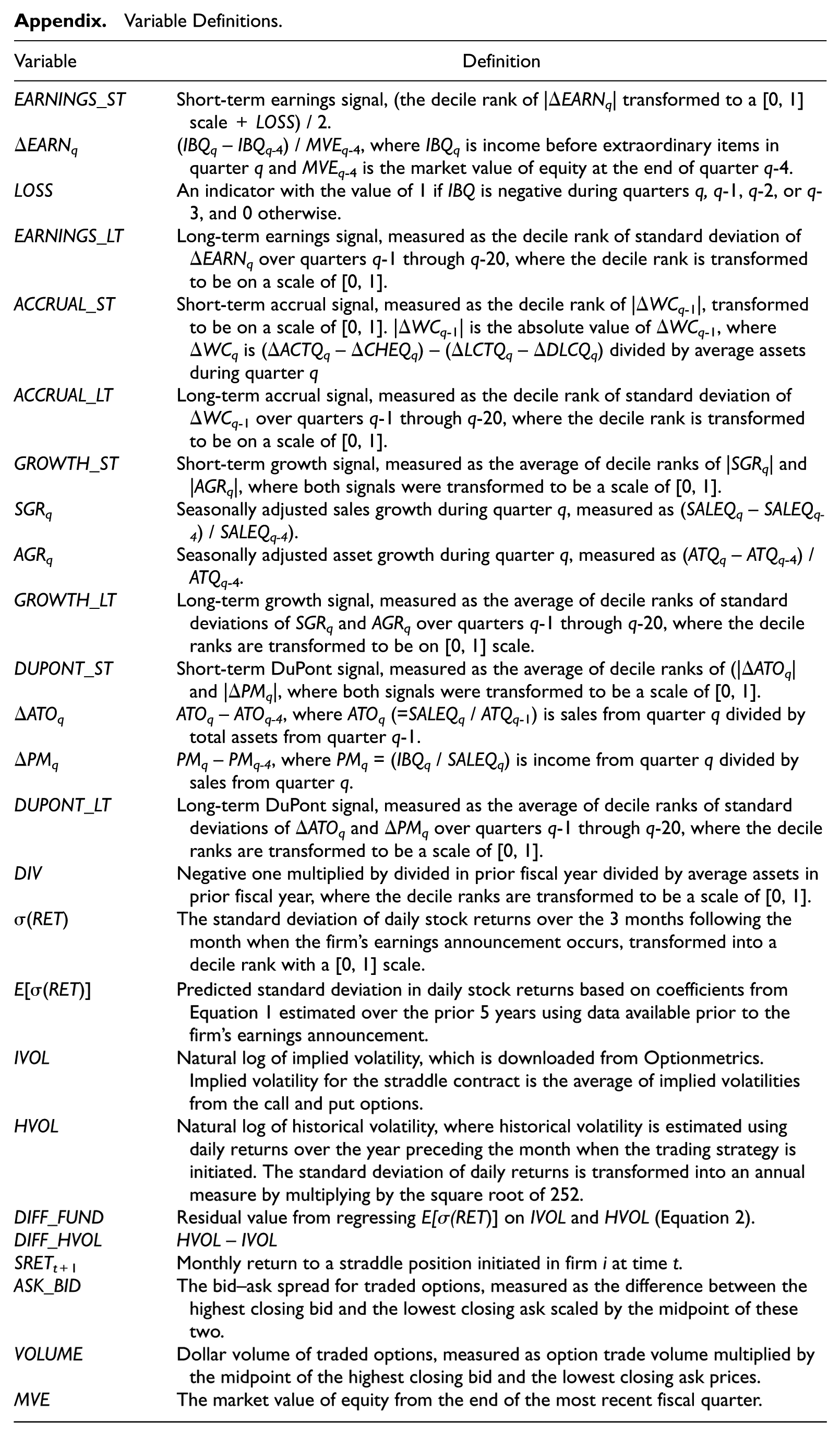
Variable Definitions.

Variable	Definition
EARNINGS_ST	Short-term earnings signal, (the decile rank of \|ΔEARN_q\| transformed to a [0, 1] scale + LOSS) / 2.
ΔEARN_q	(IBQ_q– IBQ_q-₄) / MVE_q_-4, where IBQ_q is income before extraordinary items in quarter q and MVE_q_-4 is the market value of equity at the end of quarter q-4.
LOSS	An indicator with the value of 1 if IBQ is negative during quarters q, q-1, q-2, or q-3, and 0 otherwise.
EARNINGS_LT	Long-term earnings signal, measured as the decile rank of standard deviation of ΔEARN_q over quarters q-1 through q-20, where the decile rank is transformed to be on a scale of [0, 1].
ACCRUAL_ST	Short-term accrual signal, measured as the decile rank of \|ΔWC_q_-1\|, transformed to be on a scale of [0, 1]. \|ΔWC_q_-1\| is the absolute value of ΔWC_q_-1, where ΔWC_q is (ΔACTQ_q–ΔCHEQ_q) – (ΔLCTQ_q–ΔDLCQ_q) divided by average assets during quarter q
ACCRUAL_LT	Long-term accrual signal, measured as the decile rank of standard deviation of ΔWC_q_-1 over quarters q-1 through q-20, where the decile rank is transformed to be on a scale of [0, 1].
GROWTH_ST	Short-term growth signal, measured as the average of decile ranks of \|SGR_q\| and \|AGR_q\|, where both signals were transformed to be a scale of [0, 1].
SGR_q	Seasonally adjusted sales growth during quarter q, measured as (SALEQ_q– SALEQ_q-4) / SALEQ_q-4).
AGR_q	Seasonally adjusted asset growth during quarter q, measured as (ATQ_q– ATQ_q_-4) / ATQ_q_-4.
GROWTH_LT	Long-term growth signal, measured as the average of decile ranks of standard deviations of SGR_q and AGR_q over quarters q-1 through q-20, where the decile ranks are transformed to be on [0, 1] scale.
DUPONT_ST	Short-term DuPont signal, measured as the average of decile ranks of (\|ΔATO_q\| and \|ΔPM_q\|, where both signals were transformed to be a scale of [0, 1].
ΔATO_q	ATO_q– ATO_q-4, where ATO_q (=SALEQ_q / ATQ_q_-1) is sales from quarter q divided by total assets from quarter q-1.
ΔPM_q	PM_q– PM_q-4, where PM_q = (IBQ_q / SALEQ_q) is income from quarter q divided by sales from quarter q.
DUPONT_LT	Long-term DuPont signal, measured as the average of decile ranks of standard deviations of ΔATO_q and ΔPM_q over quarters q-1 through q-20, where the decile ranks are transformed to be a scale of [0, 1].
DIV	Negative one multiplied by divided in prior fiscal year divided by average assets in prior fiscal year, where the decile ranks are transformed to be a scale of [0, 1].
σ(RET)	The standard deviation of daily stock returns over the 3 months following the month when the firm’s earnings announcement occurs, transformed into a decile rank with a [0, 1] scale.
E[σ(RET)]	Predicted standard deviation in daily stock returns based on coefficients from Equation 1 estimated over the prior 5 years using data available prior to the firm’s earnings announcement.
IVOL	Natural log of implied volatility, which is downloaded from Optionmetrics. Implied volatility for the straddle contract is the average of implied volatilities from the call and put options.
HVOL	Natural log of historical volatility, where historical volatility is estimated using daily returns over the year preceding the month when the trading strategy is initiated. The standard deviation of daily returns is transformed into an annual measure by multiplying by the square root of 252.
DIFF_FUND	Residual value from regressing E[σ(RET)] on IVOL and HVOL (Equation 2).
DIFF_HVOL	HVOL – IVOL
SRET_t ₊₁	Monthly return to a straddle position initiated in firm i at time t.
ASK_BID	The bid–ask spread for traded options, measured as the difference between the highest closing bid and the lowest closing ask scaled by the midpoint of these two.
VOLUME	Dollar volume of traded options, measured as option trade volume multiplied by the midpoint of the highest closing bid and the lowest closing ask prices.
MVE	The market value of equity from the end of the most recent fiscal quarter.

Acknowledgements

The authors thank Stan Markov (FARS [Financial Accounting and Reporting Section] discussant), Suresh Radhakrishnan (associate editor), Bharat Sarath (Editor), Cathy Schrand, Mark Trombley, an anonymous referee, and workshop participants at Cornell University, Fudan University, HKUST 2012 Accounting symposium, Yale University, The University of Texas at Dallas, University of Toronto, and the 2012 FARS conference for helpful comments and suggestions. X.F.Z thanks the Yale School of Management for financial support.

Declaration of Conflicting Interests

The author(s) declared no potential conflicts of interest with respect to the research, authorship, and/or publication of this article.

Funding

The author(s) received no financial support for the research, authorship, and/or publication of this article.

Notes

References

Abarbanell

Bushee

(1998). Abnormal returns to a fundamental analysis strategy. The Accounting Review, 73, 19-45.

Ang

Hodrick

Xing

Zhang

(2006). The cross-section of volatility and expected returns. Journal of Finance, 51, 259-299.

Ball

Brown

(1968). An empirical evaluation of accounting income numbers?Journal of Accounting Research, 6, 159-178.

Barth

M. E.

E. C.

(2014). Non-diversifiable volatility risk and risk premiums at earnings announcements. The Accounting Review, 89, 1579-1607.

Beneish

Lee

Tarpley

(2001). Contextual fundamental analysis through the prediction of extreme returns. Review of Accounting Studies, 6, 165-189.

Bernard

Thomas

(1990). Evidence that stock prices do not fully reflect the implications of current earnings for future earnings. Journal of Accounting & Economics, 13, 305-340.

Boyer

Vorkink

(2011). Stock option lotteries (Brigham Young University working paper).

Callen

(2009). Shocks to stocks: A theoretical foundation for the information content of earnings. Contemporary Accounting Research, 26, 135-166.

Choy

(2011). Retail clientele and option returns (University of Toronto working paper).

10.

Coval

Shumway

(2001). Expected option returns. Journal of Finance, 56, 983-1009.

11.

Cristoffersen

Goyenko

Jacobs

Karoui

(2011). Illiquidity premia in the equity option market (McGill University working paper).

12.

De Fontnouvelle

Fisher

Harris

. (2003). The behavior of bid-ask spreads and volume in options markets during the competition for listings in 1999. Journal of Finance, 58, 2437-2463.

13.

Dubinsky

Johannes

(2006). Fundamental uncertainty, earnings announcements, and equity options (Working paper).

14.

Fama

French

(1992). The cross-section of expected stock returns. Journal of Finance, 47, 427-466.

15.

Goyal

Saretto

(2009). Cross-section of option returns and volatility. Journal of Financial Economics, 94, 310-326.

16.

Guay

Harford

(2000). The cash-flow permanence and information content of dividend increases versus repurchases. Journal of Financial Economics, 57, 385-415.

17.

Hayn

(1995). The information content of losses. Journal of Accounting & Economics, 15, 226-244.

18.

Holthausen

Larcker

(1992). The prediction of stock returns using financial statement data. Journal of Accounting & Economics, 15, 317-411.

19.

Hong

Schoenberger

Subramanyam

K. R.

(2015). Do options price predictable patterns in future stock returns? Evidence from accounting anomalies (Working paper).

20.

Lyle

Naughton

(2016). Firm fundamentals and variance risk premiums (Working paper).

21.

Mashruwala

Rajgopal

Shevlin

(2006). Why is the accrual anomaly not arbitraged away? The role of idiosyncratic risk and transaction costs. Journal of Accounting & Economics, 42, 3-33.

22.

Maydew

(2002). Competition, market structure, and bid-ask spreads in stock option markets. Journal of Finance, 57, 931-958.

23.

Penman

(1989). Financial statement analysis and the prediction of stock returns. Journal of Accounting and Economics, 11, 295-329.

24.

Pastor

Veronesi

(2003). Stock valuation and learning about profitability. Journal of Finance, 58, 1749-1789.

25.

Penman

Reggiani

Richardson

Tuna

(2015). An Accounting-based characteristic model for asset pricing (Working paper).

26.

Piotroski

(2000). Value investing: The use of historical financial statement information to separate winners from losers. Journal of Accounting Research, 38, 1-41.

27.

Richardson

Tuna

Wysocki

(2010). Accounting anomalies and fundamental analysis: A review of recent research advances. Journal of Accounting & Economics, 50, 410-454.

28.

Rogers

Van Buskirk

Skinner

(2009). Earnings guidance and market uncertainty. Journal of Accounting & Economics, 48, 90-109.

29.

Scheinkman

Xiong

(2003). Overconfidence and speculative bubbles. Journal of Political Economy, 111, 1183-1219.

30.

Shiller

(1981). Do stock prices move too much to be justified by subsequent changes in dividends?American Economic Review, 71, 421-436.

31.

Shleifer

Vishny

(1997). The limits of arbitrage. Journal of Finance, 52, 25-55.

32.

Sloan

(1996). Do stock prices fully reflect the information in accruals and cash flows about future earnings?The Accounting Review, 71, 289-315.

33.

Soliman

(2008). The use of DuPont analysis by market participants. The Accounting Review, 83, 823-853.

34.

Sridharan

(2015). Volatility forecasting using financial statement information. The Accounting Review, 90, 2079-2106.

35.

Zhang

X. F.

(2006). Information uncertainty and stock returns. Journal of Finance, 51, 105-137.