The Value of the Tax Deferral Option

Abstract

This study explores the value of the tax deferral option. By examining ex-day stock-price-change ratios for taxable stock dividends in Taiwan, we find that the tax deferral option is valuable to investors. For a $1 taxable stock dividend, the tax deferral option produces 33.9¢ in tax savings, which suggests a tax deferral parameter of 11.3%. We also find that stocks with the tax deferral option have higher trading volumes around ex-days than those without this option, and that higher investor-level tax rates lead to higher value of the tax deferral option. We contribute to the literature by cleanly determining the value of the tax deferral option; our result is not confounded by the restart option.

Keywords

stock dividend taxation tax deferral option

Introduction

This study explores whether the tax deferral option is valuable to investors. In most countries, capital gains are taxed only when realized rather than at occurrence. This provides investors with a tax-timing option that allows them to time the realization of taxes. Under U.S. tax rules, the tax-timing option consists of two parts: the tax deferral option and the restart option.

The tax deferral option results from the realization-based taxation rule, which allows investors to defer taxes until stocks are sold (Constantinides, 1983). The restart option results from the lower tax rate of long-term gains relative to short-term gains and the offsetting rule of losses to gains, which allows investors to realize gains long-term and losses short-term via a trading strategy as proposed by Constantinides (1984).

The literature investigating the U.S. context presents mixed results¹ with respect to the importance of the restart option, which suggests that it may be the tax deferral option that drives the value of the tax-timing option. Therefore, it is crucial to explore the value of the tax deferral option. Although the tax deferral option is compatible with the conventional wisdom that investors reduce tax burdens by deferring realization of taxes, most studies focus on the restart option (e.g., Ehrhardt et al., 1995; Prisman et al., 1996), while the empirical importance of the tax deferral option is rarely explored. The scarcity of evidence motivates us to investigate this issue.

The complexity of capital gains taxation rules that include both tax deferral and restart options makes it difficult to independently determine the value of the tax deferral option. Moreover, the exercise of the tax deferral option involves no actual trading,² so it is difficult to empirically evaluate its value. To cleanly determine the value of the tax deferral option, it would be ideal to construct a research design that involves only the realization-based taxation rule, but excludes other capital gains taxation rules. The research design must also be able to account for stock pricing, facilitating estimation of the value of the tax deferral option. Unfortunately, studies exploring U.S. tax rules have difficulty meeting these conditions; however, following special stipulations in the Taiwanese tax system allows us to meet these conditions.

In Taiwan, stock dividends can be either taxable or nontaxable. In addition, the Statute of Promoting Industries Upgrading (SPIU) grants shareholders a tax deferral option on their taxable stock dividend incomes, which is based on the realization-based taxation rule that permits shareholders to defer payment of stock dividend income taxes until they sell these stock dividends. This stipulation of SPIU allows us to achieve our research purpose by contrasting the market valuations of taxable stock dividends with the tax deferral option against those without this option.

Specifically, Elton and Gruber (1970) propose a model showing that the ratio of the ex-dividend-day share-price-change amount to the dividend amount (i.e., ex-day price-change ratio, or EPCR) reflects the tax rate of the marginal investor. Accordingly, we determine the value of the tax deferral option by contrasting EPCRs of taxable stock dividends with the tax deferral option and those without this option, since on the ex-right day, any difference in the valuation implications between these two types of stock dividend can be attributed to whether they are granted with the tax deferral option.

Nevertheless, non-tax factors such as market microstructure (ex. Bali & Hite, 1998) or short-term trading (Kalay, 1982) may confound the tax interpretation of EPCR. In this regard, we determine whether taxes affect ex-day pricing behavior by contrasting EPCRs of taxable and nontaxable stock dividends. As adopted in the literature (e.g., Elton et al., 2005; Li & Weber, 2009), such a contrast-based research design helps to rule out non-tax explanations for our findings. Because, on the ex-right day, the only difference between these two types of stock dividend is in their tax treatments, any difference in their EPCRs can be clearly attributed to the effect of tax. Furthermore, taxable stock dividends produce no cash inflows, but only tax liabilities to shareholders, so tax is the most influential factor in explaining EPCRs of taxable stock dividends.

By regressing the ratio of ex-day price-change amount over the cum-right price on stock dividend yield, we estimate EPCRs for taxable and nontaxable stock dividends from the regression coefficients. We summarize our main findings as follows. First, EPCR of taxable stock dividends is significantly negative, while EPCR of nontaxable stock dividends is insignificant. This implies that tax affects ex-day stock pricing behavior, consistent with the argument of Elton and Gruber (1970). More importantly, we find that EPCR for stocks with the tax deferral option is higher than EPCR for stocks without this option; this suggests that the tax deferral option is valuable to investors.

We conduct several additional tests. First, we have a relatively small sample size for observations qualifying for the tax deferral option, and this raises the concern that our findings may suggest a special case specific to firms with particular characteristics. To address this concern, we conduct an out-of-sample test by using observations that we cannot classify as to whether they qualify for the tax deferral option. We first run a logistic regression to estimate the probability of qualifying for the tax deferral option for each of these observations. We then repeat our EPCR tests by using this estimated probability to identify the qualification status. We find that this two-stage test does not change our conclusion; this suggests that our finding can generalize to a broader population.

In addition, we explore how the tax deferral option affects trading volume around ex-right days. If the tax deferral option is indeed valuable to investors, it should affect investor trading behavior, as reflected on trading volume. We find that, compared with stocks without the tax deferral option, stocks with this option have higher excess trading volumes for either the cum-right period or the ex-right period. This result suggests the impact of the tax deferral option on investor trading behavior.

Finally, we examine whether investor-level tax rates affect the valuation of the tax deferral option. This is a difficult task because information regarding investor tax status is usually unavailable. We overcome this difficulty by exploiting the unique stock ownership data provided by the Taiwan Economic Journal (TEJ) database to construct a cross-sectional proxy that measures the firm-level weighted average tax rate (WAT) of shareholders. We find that higher WAT is associated with larger difference in EPCRs between qualified and nonqualified firms; this finding suggests that a higher investor tax rate leads to a higher value of the tax deferral option.

Our study makes the following contributions to the literature. First, we show that the tax deferral option is valuable and this result is not confounded by the restart option. Our study is critical because prior studies usually base their research designs on investigating U.S. tax rules and this leads their results to reflect both effects of restart and tax deferral options. In this regard, our study helps to resolve the under-explored issue about the value of the tax deferral option.

Our study generates a new estimate of the tax deferral parameter, 11.3%.³ Our study also provides a monetary estimate of the valuation for the tax deferral option. For a $1 taxable stock dividend, the tax deferral option results in a 33.9¢ tax savings. Such substantial tax savings suggest that the realization-based taxation rule (i.e., taxes are recognized when stock dividends are sold) results in significantly lower tax burdens for investors than does the incurrence-based taxation rule (i.e., taxes are recognized when stock dividends incur), where the former applies to taxable stock dividends with the tax deferral option and the latter applies to those without this option.

Our study also shows that tax status affects how investors value the tax deferral option. Our result implies that a 1% increase in investor-level tax rate produces a 6.8¢ increase in the value of the tax deferral option. Therefore, investor tax status is a determinant for the value of the tax deferral option. This result is crucial because there is little evidence showing what factors determine the value of the tax deferral option.

Finally, we contribute to the ex-day stock pricing literature by showing that EPCR reflects the effect of taxes. It is still controversial to date whether taxes can explain ex-day stock price changes (e.g., Bali & Hite, 1998; Kalay, 1982). We find significant EPCR for taxable stock dividends but insignificant EPCR for nontaxable stock dividends. This finding suggests that taxes have a first-order effect on explaining ex-day stock price changes.

This article proceeds as follows. Section “Stock Dividend Regulations and Taiwan’s Tax System” reviews the tax system and stock dividend regulations in Taiwan. Section “Model and Hypothesis Development” develops our theoretical model and empirically testable hypothesis. Section “Empirical Methodology” presents our research methodology and sample selection. Section “Empirical Results” sets forth the empirical results. Section “Additional Analysis” presents additional empirical analyses. Finally, Section “Conclusion” describes our conclusions.

Stock Dividend Regulations and Taiwan’s Tax System

Stock Dividend Regulations

In Taiwan, the Company Law stipulates that stock dividends can be distributed from retained earnings or from capital surplus, where firms determine from which source stock dividends are distributed. Stock dividends distributed from capital surplus are deemed as a return of capital and thus nontaxable, while those distributed from retained earnings are viewed as a distribution of profits and thus taxable. The legally defined par value per share is NT$10. If we define the NT-dollar amount of the stock dividend as S, then the shareholder receives S divided by 10 additional shares for each initial share owned and incurs tax liability equal to S multiplied by the shareholder’s income tax rate, where S is viewed as income, like cash dividends. Stock dividend taxes depend on the amount of S declared rather than on stock price.⁴ In addition, Taiwanese firms announce dividends yearly rather than quarterly.

The tax deferral option for stock dividend incomes is stipulated in Article 16 of the SPIU.⁵ Briefly, Article 16 stipulates that if firms distribute stock dividends from retained earnings (i.e., taxable stock dividends) and designate those retained earnings as funding sources for specific purposes (mainly related to equipment investments, R&D activities, or investments in other companies within specific industries), they can apply for the Ministry of Economic Affairs and the tax authorities to grant those taxable stock dividends with the option to defer shareholder income taxes.

When the applications are approved, firms will inform shareholders that the stock dividends they receive are granted with the tax deferral option and shareholders can thus identify which shares are not taxed until sold. As in Taiwan all stocks issued, including stock dividends distributed, are inscribed stocks, sales of stock dividends with the tax deferral option will be perceived by firms, given that the transfer of inscribed stocks requires firms to change shareholder names on the shareholder registers. Firms are mandated to notify tax authorities these sales, allowing tax authorities to levy income taxes on these stock dividends.

With the tax deferral option, taxable stock dividends are subjected to income taxes when they are sold rather than when they incur, so shareholders can decide when to realize tax payments by timing the sale of those stock dividends. Moreover, in a specific year, if the firm conforms to Article 16, then the tax deferral option is applicable to all taxable stock dividends declared in that year; otherwise, all stock dividends are taxed immediately, like cash dividends.

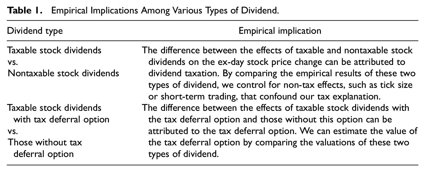
Table 1 summarizes the empirical implications for different types of stock dividend.

Table 1.

Empirical Implications Among Various Types of Dividend.

Dividend type	Empirical implication
Taxable stock dividends vs. Nontaxable stock dividends	The difference between the effects of taxable and nontaxable stock dividends on the ex-day stock price change can be attributed to dividend taxation. By comparing the empirical results of these two types of dividend, we control for non-tax effects, such as tick size or short-term trading, that confound our tax explanation.
Taxable stock dividends with tax deferral option vs. Those without tax deferral option	The difference between the effects of taxable stock dividends with the tax deferral option and those without this option can be attributed to the tax deferral option. We can estimate the value of the tax deferral option by comparing the valuations of these two types of dividend.

Prior studies propose several reasons why firms distribute stock dividends. For example, Grinblatt et al. (1984) argue that stock splits or stock dividends contain information about future firm performance. Lakonishok and Lev (1987) and McNichols and Dravid (1990) argue that stock splits can realign stock prices to optimal ranges and boost a stock’s liquidity. However, these studies explore an environment where stock dividend is tax free, so they cannot explain why firms distribute taxable stock dividends that saddle shareholders with a tax liability without producing real incomes. In this regard, Kuo and Lee (2013) and Kuo (2012) argue that taxable stock dividends incur managers (i.e., controlling shareholders in Taiwan) with large taxes so they can signal managerial confidence about future firm performance.⁶ Consistent with this signaling argument, Kuo and Lee (2013) find that managers’ shareholdings are positively associated with market reactions to announcements of taxable stock dividends, which suggest that investors perceive the signaling value of taxable stock dividends.

Note that the signaling argument does not affect our empirical results because the information content of taxable stock dividends (signaling effect) should have been absorbed by the market around announcement days, suggesting that it will not confound stock pricing behaviors on subsequent days such as ex-right days. This is also why we explore ex-day stock pricing, because trading around ex-days less likely results from differences in information such as signaling but most likely from tax-induced valuation.

Features of Taiwan’s Tax System

For individual taxpayers, incomes from dividends and other sources are combined into a single consolidated income, which is subjected to progressive income tax rates of 6%, 13%, 21%, 30%, and 40%, such that the marginal dividend tax rate is equal to the applicable income tax rate. For domestic corporate shareholders, the corporate income tax rate is set at 25%,⁷ and the dividend-received deduction is 80%. The real dividend income tax rate for domestic corporate investors is thus 25% × (1–80%) = 5%. Foreign shareholders, either individual or corporate, face essentially a withholding tax rate of 20% on their dividend incomes.

Capital gains taxes on securities trading have not been levied since January 1, 1990. Therefore, the only tax that taxable stock dividends are subjected to is the income tax, which can be deferred by the option stipulated in SPIU. Shareholders cannot covert the tax deferral option granted to stock dividends into a restart option by selling these stock dividends and then repurchasing them, because the repurchased stocks will not be subjected to capital gains taxes when they are sold.

The tax rate applicable to taxable stock dividend income is the shareholder’s income tax rate, and taxable income is essentially constant at the legal par value NT$10 for every share of stock dividend received, regardless of the length of the holding period and subsequent change in share prices. Therefore, dividend tax liabilities are determinable before a stock goes ex-right.

Tax Deferral Option and Restart Option

For expositional purpose, we use the following essential rules of the U.S. tax code to illustrate the tax deferral and the restart options: (1) capital gains taxes are recognized when gains are realized, rather than when they occur; (2) the tax rate is higher for short-term capital gains than for long-term capital gains; and (3) the offsetting rule stipulates that losses can offset gains, and net short-term losses must be used to offset net long-term gains before applying any tax rate.

These rules result in the tax-timing option, which includes two parts. The first is the tax deferral option, which is based on Rule 1 and is compatible with conventional wisdom that investors reduce taxes by deferring the realization of gains (Constantinides, 1983). Hence, the realization-based taxation rule is the basis of the tax deferral option. This justifies our examination of the tax option stipulated in SPIU because it is also built on a realization-based taxation rule (i.e., stock dividend incomes are not taxed until sold).

The second part is the restart option (Constantinides, 1984), which is based on Rules 2 and 3 and allows investors to reduce taxes by continually adjusting portfolios to realize long-term gains by selling and immediately repurchasing an asset to increase tax basis, and restarting the option to realize future losses short term. If the tax rate for long-term realizations is lower relative to short-term realizations, the tax cost of recognizing long-term gains could be smaller than the value of the option to take future losses short term. Therefore, a potential tax advantage is created by recognizing a long-term gain and paying the tax.

The generalizability of the restart option is questioned by Dammon et al. (1989) because it heavily depends on the pattern of realized returns, and the return pattern studied by Constantinides (1984) may not represent a typical one. This seems to imply that the value of the tax-timing option is primarily determined by the tax deferral option. However, it is difficult to independently estimate the value of the tax deferral option by exploring U.S. tax rules.

By examining the Taiwanese market, we can determine the value of the tax deferral option without being confounded by the restart option, because Article 16 of SPIU is based on the realization-based taxation rule, as stipulated in Rule 1 and is unrelated to Rules 2 and 3. In particular, capital gains on security trading are tax free in Taiwan so the only tax relevant to stock dividends is the income tax. Holding period will not affect the tax rate applicable to stock dividend incomes because the idea of distinguishing long-term versus short-term tax rates is not applicable to income tax. The offsetting rule is also not applicable to the taxation of stock dividend incomes because their tax basis is constant at the legal par value, which makes the idea of distinguishing losses and gains irrelevant.

Model and Hypothesis Development

This section clarifies how we follow the Elton and Gruber (1970; EG hereafter) model to explore EPCR to determine the value of the tax deferral option. The EG model assumes that the marginal investor is risk neutral, there is no information uncertainty in the market, and transaction costs are trivial and can be neglected. We extend the EG model to accommodate the taxable stock dividend case. Our analysis considers two types of trader: a representative seller and a representative buyer. Following EG, the representative seller (buyer) is a long-term trader who have already decided to sell (buy) the stock such that his only remaining decision around ex-right days is whether to transact before or after the stock goes ex-right.⁸

The EG model suggests that market prices will be in equilibrium if sellers (buyers) are indifferent between selling (buying) the share before or after it goes ex-right. Equation 1 shows the indifferent condition for sellers between selling the share before or after the ex-right day:

P_{c} = P_{e} \cdot (1 + L) - S_{T} \cdot t_{d},

(1)

where P_c is the cum-right price; P_e is the ex-right price; S_T (S_NT) is the taxable (nontaxable) stock dividend per share; t_d is the representative investor’s marginal tax rate on dividend incomes; and L = (S_T+S_NT)/10, in which L represents the number of additional shares per initial share received from stock dividends.⁹ The left-hand side of Equation 1 represents cash flow when selling on the last cum-right day, and the right-hand side represents cash flow when selling on the first ex-right day. Using the same logic of Equation 1, the indifferent condition for buyers is shown in Equation 2:

- P_{c} - S_{T} \cdot t_{d} = - P_{e} \cdot (1 + L) .

(2)

The equilibrium condition requires both Equations 1 and 2 to hold simultaneously. By comparison, we recognize that the indifferent condition for sellers is identical to that for buyers, so rearranging Equation 1 or 2 leads to EPCR for stock dividends without the tax deferral option (EPCR_without), as shown in Equation 3:

EPC R_{without} = \frac{P_{c} - P_{e} \cdot (1 + L)}{S_{T}} = - t_{d} .

(3)

Equation 3 shows that EPCR reflects the representative investor’s tax rate t_d. Contrasting with EPCR for cash dividends as illustrated in Elton and Gruber (1970), EPCR for taxable stock dividends is negative because stock dividends produce no cash inflows. Hence, the ex-right share value P_e·(1 + L) must be higher than cum-right share value, P_c, to compensate for taxes on stock dividends t_d·S_T (Dhatt et al., 1993).

To express how the tax deferral option affects EPCR, we set OP to represent the effect of the tax deferral option. With the tax deferral option, the dividend tax rate reduces from t_d to (t_d − OP). The EPCR for stock dividends with the tax deferral option (EPCR_with hereafter) is:

EPC R_{with} = \frac{P_{c} - P_{e} \cdot (1 + L)}{S_{T}} = - (t_{d} - OP),

(4)

where OP is the tax-reduction factor resulting from the tax deferral option. Conceptually, OP captures the value of the tax deferral option. A larger OP represents greater savings from the present value of the tax payment since the effect of delaying taxation is similar to discounting the tax liability that is payable immediately. Consequently, the effective tax rate reduced from t_d to t_d − OP.

By contrasting the pricing difference between EPCR_with and EPCR_without, our empirical test can determine the value of the tax deferral option, where we expect that EPCR_with > EPCR_without. Based on analysis above, we present the following hypothesis:

Hypothesis: Ceteris paribus, stocks qualified for the tax deferral option have higher (i.e., less negative) EPCR than do stocks not qualified for that option.

For expositional purpose, we view OP as a constant and subtract it from t_d in Equation 4. However, OP is actually a function of t_d. We discuss this point in Section “Further discussion for the relation between tax deferral option and EPCR.”

Empirical Methodology

Regression Specification

Elton and Gruber (1970) employ the average of raw EPCRs to explore ex-day stock pricing behavior. However, this suffers from the heteroskedasticity problem because raw EPCR is scaled by dividends and this exacerbates ex-day price movements for tiny dividends (Michaely, 1991).¹⁰ To address this concern, we conduct our tests by regressing the ratio of ex-right day price change to the cum-right price (P_c − P_e(1 + L))/P_c on taxable stock dividend yield S_T/P_c. Specifically, by moving S_T to the right-hand side and then denominating P_c on both sides, Equations 3 and 4 can be rearranged as Equations 5.1 and 5.2, respectively:

\frac{P_{c} - P_{e} \cdot (1 + L)}{P_{c}} = - t_{d} \cdot \frac{S_{T}}{P_{c}},

(5.1)

\frac{P_{c} - P_{e} \cdot (1 + L)}{P_{c}} = - (t_{d} - OP) \cdot \frac{S_{T}}{P_{c}} .

(5.2)

Equation 5.1 suggests that by regressing (P_c − P_e(1 + L))/P_c on S_T/P_c, EPCR_without (−t_d) can be estimated from the regression coefficient of S_T/P_c. Equation 5.2 also suggests that EPCR_with (−(t_d− OP)) can be estimated with the same regression specification. As shown in Bell and Jenkinson (2002), this regression specification mitigates the heteroskedasticity problem because now we can estimate EPCR without scaling it with dividends (Brown & Clarke, 1993; Cloyd et al., 2006; Li & Weber, 2009). This also suggests that using this regression specification with a sample pooling observations qualified for the tax deferral option and those not qualified, the value of the tax deferral option can be estimated with the difference in the regression coefficient of S_T/P_c between these two groups of observations.

We use the following regression in Equation 6 to examine our hypothesis:

\begin{matrix} {(\frac{P_{c} - P_{e} \cdot (1 + L)}{P_{c}})}_{it} = α + β_{1} \cdot {(\frac{S_{T}}{P_{c}})}_{it} + β_{2} \cdot {(\frac{S_{NT}}{P_{c}})}_{it} + β_{3} \cdot DUM I_{it} \\ + β_{4} \cdot {(\frac{S_{T}}{P_{c}})}_{it} \cdot DUM I_{it} + β_{5} \cdot {(\frac{S_{NT}}{P_{c}})}_{it} \cdot DUM I_{it} + β_{k} \cdot X_{kit} + η_{it}, \end{matrix}

(6)

where P_c and P_e are the cum-right day closing price and ex-right day closing price,¹¹ respectively;¹²S_T and S_NT are the amounts of taxable and nontaxable stock dividends, respectively; L is the stock dividend payout ratio, which equals (S_T+S_NT)/10; DUMI_it = 1 if observation i in year t is qualified for the tax deferral option stipulated in Article 16 of SPIU, and 0 otherwise; X_kit is a vector of control variables, controlling for factors influential on ex-right day stock pricing; α and β_j are the intercept and regression coefficients, respectively; and η_it is the error term. The standard errors of coefficients are calculated following the procedure of Newey and West (1987).

β₁ and β₂ represent the EPCRs for taxable and nontaxable stock dividends, respectively. Based on Equation 5.1, we expect β₁ to be negative. As clarified in Table 1, observing a difference between β₁ and β₂ rules out the confounding effects of non-tax factors. If tax is not the primary factor of EPCR, then β₁ and β₂ should show no difference (i.e., both of their coefficients are significant or insignificant and have similar magnitude).

To examine our hypothesis, we identify which firms are qualified for the tax deferral option based on the firm list in Guo (1996), whose data are from the Ministry of Finance. This firm list spans the period 1991 to 1996 and shows which firms are granted the tax deferral option. We also search from the internet about which firms ever disclose that they are qualified for the tax deferral option. Based on these data, we construct our identification variable DUMI, which indicates whether a firm is qualified for the tax deferral option in any specific year during 1991 to 1996.

Our hypothesis argues that EPCR for taxable stock dividends is higher for observations qualified for the tax deferral option than for those not qualified. Theoretically, the coefficient of S_T/P_c·DUMI represents the value of the tax deferral option because it captures the difference in the coefficient of S_T/P_c between qualified and nonqualified observations and Equations 5.1 and 5.2 show that this difference equals OP. We thus expect β₄ to be positive, which suggests that the tax deferral option is valuable.

Although Equations 5.1 and 5.2 do not suggest an intercept, Boyd and Jagannathan (1994) and Frank and Jagannathan (1998) develop microstructure models that imply a nonzero intercept in the regression of ex-day stock pricing. If such microstructure effects were pronounced, then forcing the intercept to zero would bias the estimate of regression coefficients. We thus include an intercept in Equation 6. We also include the stand-alone effect of DUMI to control for the possibility that microstructure effects might have differential influences on qualified firms than on nonqualified firms. The inclusion of DUMI also avoids that microstructure effects confound our interpretation of S_T/P_c·DUMI.

Exploring S_T/P_c·DUMI mitigates the endogenous concern that a reverse causality from EPCR to DUMI may arise because firms may adapt their applications for the tax deferral option to cater to investor tax status. In this regard, focusing on the interaction effect makes it difficult to argue for such reverse causality. Moreover, we include S_NT/P_c·DUMI in Equation 6 because this allows us to contrast S_T/P_c·DUMI with S_NT/P_c·DUMI, which helps to rule out the confounding explanation that β₄ reflects the effect of some non-tax firm characteristics systematically related to qualification status for the tax deferral option. This is because any difference between these two interaction terms can be attributed to the effect of the tax deferral option.

Referring to Li and Weber (2009), we include the following control variables in Equation 6: ROE measures firm profitability, defined as net income divided by total equity; Growth is the average sales growth rate over the preceding 2 years; Turnover is the stock trading turnover ratio on the ex-right day, defined as daily share trading volume to total shares outstanding; Illiquidity measures stock liquidity (Amihud, 2002), which is the annual average of the absolute value of daily stock return to dollar trading volume; Size is the natural log of total assets; Debt is the ratio of total liabilities to total assets; and STD is the standard deviation of daily stock return over the 250-day period preceding the ex-right day. Except for STD and Turnover, all control variables are measured as of the preceding year-end relative to the ex-right day.

One potential confounding interpretation regarding S_T/P_c and S_NT/P_c is that their effects arise from firm characteristics associated with stock dividend payout decisions. Therefore, we include ROE, Growth, and Debt, as firm profitability, growth potential, and capital structure are shown to affect stock dividend payout decisions (Kuo, 2012). Moreover, Michaely and Vial (1996) argue that transaction costs may affect investor trading willingness and thus affect ex-day stock pricing behavior. Hence, we include Illiquidity because more liquid stocks typically have lower transaction costs.¹³ Similarly, we include Size because larger firms are often more liquid and this also controls for any size effect (Lasfer, 2008; Naranjo et al., 2000). We include STD to control for the effects of firm idiosyncratic risk on stock returns (Fu, 2009; Merton, 1987). Finally, we include Turnover to control for the potential effect of trading volume on stock price changes since an extensive literature finds a positive association between them (see Karpoff, 1987, for a review of explanations).

Sample Selection

Using data from TEJ, our sample period spans 1991 to 1996. We choose this period to correspond to Guo’s (1996) firm list. We initially include all firms listed on the Taiwan Stock Exchange that declared dividends during our sample period. This generates 1,607 observations. To avoid the confounding effect of cash dividends, we exclude 132 observations that declare both cash and stock dividends and have the same ex-dividend and ex-right days. We omit 11 observations with ex-right stock prices higher than or equal cum-right stock prices because, in theory, cum-right prices should be higher.¹⁴ The higher ex-right prices suggest that they could be contaminated by events or news unrelated to our study. We eliminate seven observations with incomplete data to estimate Equation 6.

As Guo’s (1996) firm list does not cover all listed firms, to avoid measurement error, we omit 798 observations for which we cannot determine whether they qualify for the tax deferral option, so our sample covers only firm–year observations for which we can identify qualification status. Furthermore, we identify observations that declare only nontaxable stock dividends as not qualified for the tax deferral tax option, because Article 16 of SPIU applies only to taxable stock dividends. Therefore, firms qualified for the tax deferral option are unlikely to declare only nontaxable stock dividends, but they are likely to announce only taxable stock dividends or a mix of both types of stock dividend. Based on above selection procedures, our sample contains 659 firm–year observations, among which 59 observations are qualified for the tax deferral option and the remaining 600 are not qualified.¹⁵

Empirical Results

Descriptive Statistics

Industry distribution of the sample is shown in Table 2.

Table 2.

Industry Distribution of Sample.

Industry	Panel A: sample with tax deferral option			Panel B: sample without tax deferral option
	Total	TO	Both	Total	TO	NTO	Both
Electronics	9	9	0	42	6	16	20
Electric machinery	2	0	2	19	9	3	7
Chemicals	2	1	1	42	14	13	15
Automobiles	0	0	0	6	1	3	2
Cement	6	4	2	17	5	3	9
Food	2	1	1	60	3	31	26
Plastics	12	9	3	28	22	1	5
Textiles	9	5	4	64	16	24	24
Electronic appliances	0	0	0	43	3	19	21
Glass and china	0	0	0	2	0	2	0
Paper	2	1	1	21	2	9	10
Steel	1	1	0	44	4	36	4
Rubber	2	2	0	20	7	5	8
Construction	1	1	0	36	3	15	18
Transportation	3	1	2	19	3	8	8
Tourism	0	0	0	18	0	9	9
Finance	3	1	2	61	15	2	44
General merchandise	2	0	2	22	2	11	9
Gas and oil	0	0	0	4	1	3	0
Other	3	3	0	32	9	9	14
Total	59	39	20	600	125	222	253

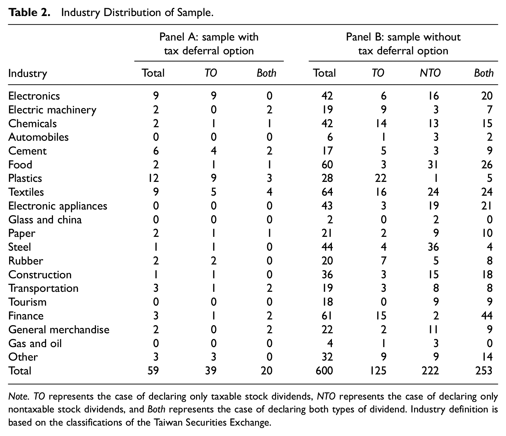
Note. TO represents the case of declaring only taxable stock dividends, NTO represents the case of declaring only nontaxable stock dividends, and Both represents the case of declaring both types of dividend. Industry definition is based on the classifications of the Taiwan Securities Exchange.

In Table 2, Panels A and B report cases for observations qualified for the tax deferral option and those not qualified, respectively. The proportion of observations that declare only taxable stock dividends is 66% (39/59) in Panel A, while in Panel B this proportion is only 33% (125/(125 + 253). This suggests that qualified firms are inclined to declare more taxable stock dividends; this may be because the tax deferral option mitigates the influence of shareholder tax consequences on firms’ decisions to declare taxable stock dividends.

Several results in Panel A of Table 2 are noteworthy. First, qualified firms tend to cluster in particular industries (e.g., electronics or plastics); this raises the concern that the effect of the tax deferral option may reflect attributes of these industries. To alleviate this concern, we control for industry fixed effects in Equation 6. Second, most qualified firms are in manufacturing industries, but there are some qualified firms in non-manufacturing industries (finance and general merchandise), where non-manufacturing corporations can apply Article 16 of SPIU by investing in other corporations that are within industries defined in Article 8.

Table 3 presents the descriptive statistics.

Table 3.

Descriptive Statistics.

	ΔP/P_c	S_T	S_NT	ROE	Growth	Illiquidity	Size	Debt	Turnover	STD	S_T/P_c	S_NT/P_c
Panel A: full sample
Mean	−0.010	0.818	0.656	0.090	0.272	1.151	6.917	0.419	1.431	2.357	0.015	0.017
Median	−0.010	0.569	0.500	0.085	0.086	0.029	6.790	0.385	0.974	2.229	0.013	0.014
Standard deviation	0.032	1.048	0.627	0.084	2.573	7.993	0.601	0.203	1.519	0.678	0.015	0.015
25% Quartile	−0.028	0.000	0.010	0.037	0.010	0.015	6.503	0.289	0.472	1.909	0.000	0.000
75% Quartile	0.005	1.200	1.000	0.132	0.178	0.052	7.208	0.511	1.874	2.596	0.024	0.027
Panel B: sample with tax deferral option
Mean	−0.006	1.524	0.275	0.142	0.105	1.843	7.108	0.382	0.974	2.278	0.026	0.006
Median	−0.007	1.000	0.000	0.124	0.100	0.027	7.170	0.362	0.545	2.179	0.022	0.000
Standard deviation	0.028	1.652	0.521	0.089	0.155	6.757	0.574	0.147	1.057	0.732	0.017	0.009
25% Quartile	−0.019	0.650	0.000	0.099	0.003	0.012	6.620	0.287	0.148	1.693	0.016	0.000
75% Quartile	0.008	1.600	0.500	0.159	0.143	0.048	7.540	0.481	1.421	2.609	0.030	0.011
Panel C: sample without tax deferral option
Mean	−0.010	0.749	0.694	0.085	0.288	1.083	6.898	0.423	1.476	2.365	0.014	0.018
Median	−0.011	0.500	0.600	0.078	0.085	0.029	6.780	0.388	1.011	2.233	0.012	0.016
Standard deviation	0.032	0.940	0.624	0.081	2.695	8.106	0.601	0.207	1.549	0.672	0.015	0.015
25% Quartile	−0.029	0.000	0.200	0.034	0.010	0.015	6.497	0.289	0.510	1.922	0.000	0.003
75% Quartile	0.005	1.100	1.000	0.129	0.180	0.053	7.171	0.513	1.897	2.589	0.024	0.028

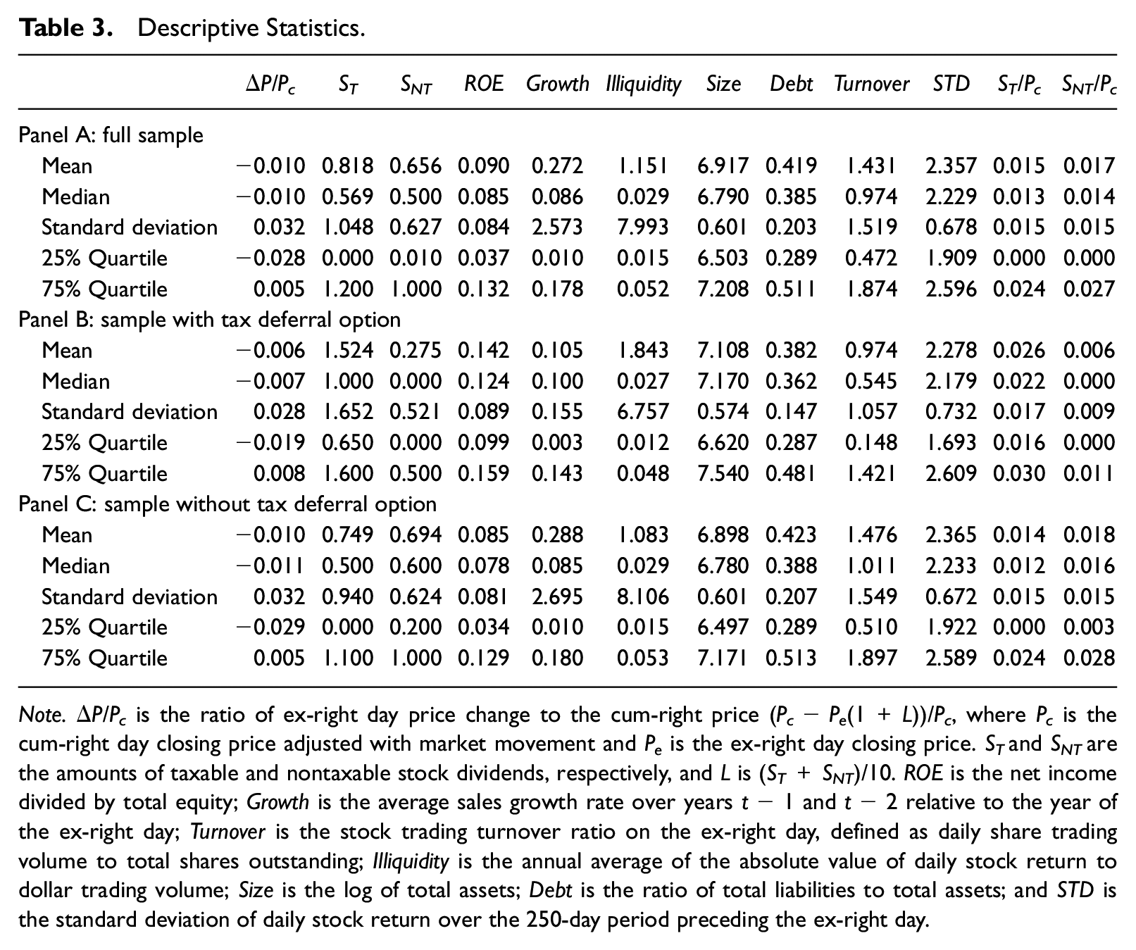
Note.ΔP/P_c is the ratio of ex-right day price change to the cum-right price (P_c − P_e(1 + L))/P_c, where P_c is the cum-right day closing price adjusted with market movement and P_e is the ex-right day closing price. S_T and S_NT are the amounts of taxable and nontaxable stock dividends, respectively, and L is (S_T+S_NT)/10. ROE is the net income divided by total equity; Growth is the average sales growth rate over years t − 1 and t − 2 relative to the year of the ex-right day; Turnover is the stock trading turnover ratio on the ex-right day, defined as daily share trading volume to total shares outstanding; Illiquidity is the annual average of the absolute value of daily stock return to dollar trading volume; Size is the log of total assets; Debt is the ratio of total liabilities to total assets; and STD is the standard deviation of daily stock return over the 250-day period preceding the ex-right day.

In Table 3, Panel A reports the descriptive statistics of the full sample, and Panels B and C report the descriptive statistics of sample with and without the tax deferral option, respectively. As shown in Panels B and C, firms qualified for the tax deferral option have higher mean and median of ΔP/P_c, (P_c − P_e(1 + L))/P_c, than firms not qualified, which suggests that the tax deferral option decreases the premium (i.e., the difference between P_e(1 + L) and P_c) investors require to compensate for taxes. Moreover, firms qualified for the tax deferral option have higher mean and median of S_T but lower mean and median of S_NT. This result is largely consistent with Table 2 in that the tax deferral option may affect firms’ decisions to declare taxable stock dividends.

Table 4 presents the correlation matrix, where Pearson’s correlations are reported above the diagonal and Spearman’s correlations are reported below the diagonal. The correlation between ΔP/P_c and S_T/P_c is significantly negative for both Person’s and Spearman’s correlations. In contrast, the correlation between ΔP/P_c and S_NT/P_c is insignificant for either case. This provides preliminary evidence suggesting that EPCR for taxable stock dividends is negative and reflects the effect of taxes. As a robustness check, we find that all the variance inflation factors for variables in Equation 6 are less than 2.5, suggesting that multicollinearity seems not a serious concern.

Table 4.

Correlation Matrix.

	ΔP/P_c	DUMI	S_T/P_c	S_NT/P_c	ROE	Growth	Illiquidity	Size	Debt	Turnover	STD
ΔP/P_c		.0373	−.1209	.0388	−.1643	−.0211	.0468	−.1732	−.0708	−.1314	−.0777
		(.3393)	(.0019)	(.3203)	(.0001)	(.5894)	(.2300)	(.0001)	(.0694)	(.0007)	(.0463)
DUMI	.0490		.2227	−.2220	.1961	−.0203	.0272	.1001	−.0581	−.0944	−.0369
	(.2092)		(.0001)	(.0001)	(.0001)	(.6021)	(.4865)	(.0101)	(.1364)	(.0153)	(.3447)
S_T/P_c	−.1525	.2224		−.4251	.4998	.0148	−.0663	.1466	−.0741	−.1051	−.1896
	(.0001)	(.0001)		(.0001)	(.0001)	(.7045)	(.0891)	(.0002)	(.0572)	(.0070)	(.0001)
S_NT/P_c	.0418	−.2546	−.5260		−.3580	.0666	.0447	−.1457	−.0459	.1344	−.0769
	(.2834)	(.0001)	(.0001)		(.0001)	(.0877)	(.2519)	(.0002)	(.2396)	(.0005)	(.0485)
ROE	−.1652	.2033	.5701	−.4773		.1238	−.0334	.3507	.1340	−.0768	−.1377
	(.0001)	(.0001)	(.0001)	(.0001)		(.0015)	(.3925)	(.0001)	(.0006)	(.0487)	(.0004)
Growth	−.0703	−.0168	.1929	−.0502	.3337		−.0111	−.0415	−.0591	.0131	−.0181
	(.0713)	(.6670)	(.0001)	(.1985)	(.0001)		(.7764)	(.2872)	(.1294)	(.7375)	(.6436)
Illiquidity	.2679	−.0261	−.2870	.1522	−.4288	−.2187		−.1494	.0250	−.1050	.0587
	(.0001)	(.5030)	(.0001)	(.0001)	(.0001)	(.0001)		(.0001)	(.5225)	(.0070)	(.1320)
Size	−.1183	.1256	.1702	−.0699	.3325	.1610	−.6395		.6664	−.1742	−.2297
	(.0023)	(.0012)	(.0001)	(.0730)	(.0001)	(.0001)	(.0001)		(.0001)	(.0001)	(.0001)
Debt	−.0507	−.0436	−.1110	.0650	.0450	.2260	−.2017	.4881		−.0035	−.0470
	(.1933)	(.2642)	(.0043)	(.0956)	(.2483)	(.0001)	(.0001)	(.0001)		(.9281)	(.2286)
Turnover	−.1896	−.1381	−.0952	.1783	−.1295	.0889	−.0979	−.2062	.0201		.1436
	(.0001)	(.0004)	(.0145)	(.0001)	(.0009)	(.0224)	(.0119)	(.0001)	(.6071)		(.0002)
STD	−.0908	−.0432	−.2213	−.0210	−.2053	−.0573	.1284	−.2793	−.0109	.3010
	(.0198)	(.2677)	(.0001)	(.5913)	(.0001)	(.1420)	(.0010)	(.0001)	(.7810)	(.0001)

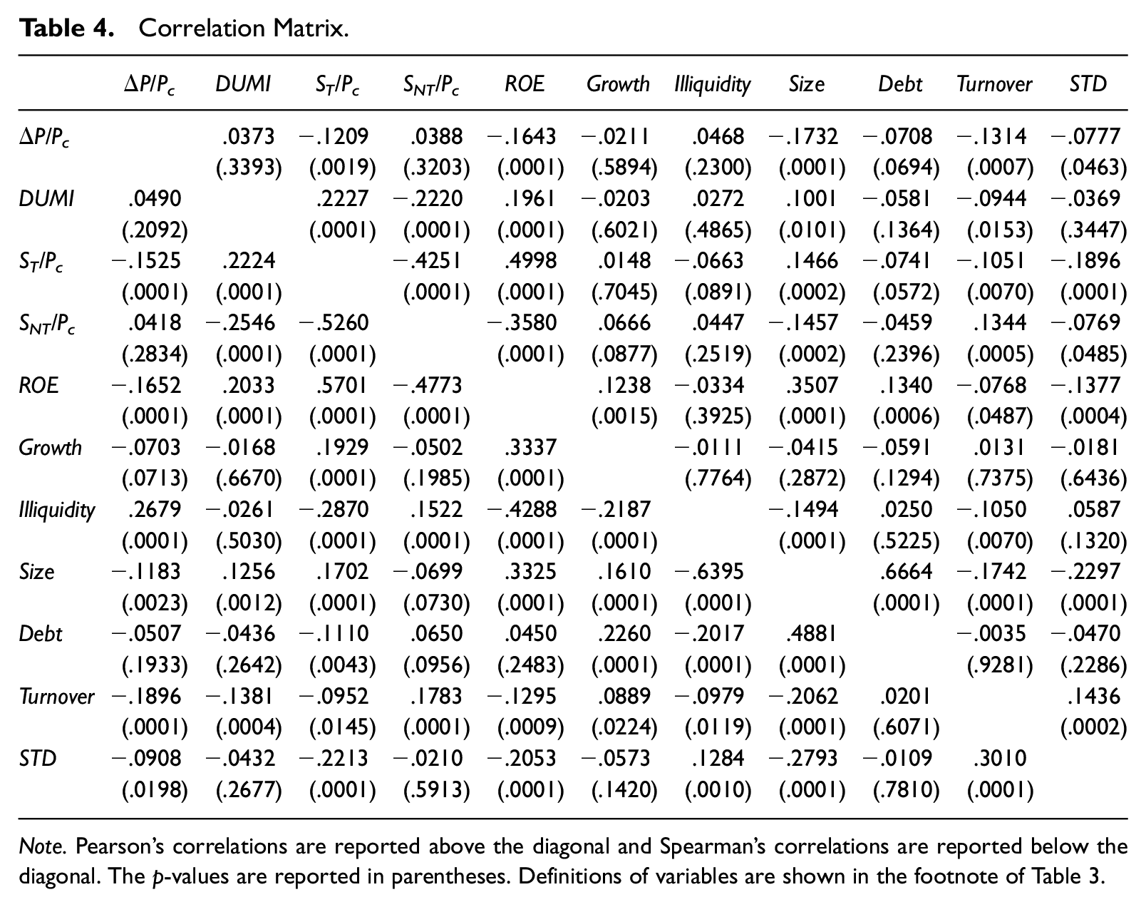
Note. Pearson’s correlations are reported above the diagonal and Spearman’s correlations are reported below the diagonal. The p-values are reported in parentheses. Definitions of variables are shown in the footnote of Table 3.

Value of the Tax Deferral Option

Table 5 shows our main empirical results from estimating Equation 6.

Table 5.

Estimate Results of Equation 6.

	Column 1		Column 2		Column 3
	Coefficient	p-value	Coefficient	p-value	Coefficient	p-value
Constant	−.006	.097*	.151	.000***	.148	.000***
S_T/P_c	−.286	.001***	−.347	.000***	−.382	.000***
S_NT/P_c	−.010	.914	−.129	.143	−.121	.187
DUMI	.008	.030**	.008	.026**	.002	.807
S_T/P_c × DUMI					.339	.043**
S_NT/P_c × DUMI					−.395	.340
ROE			−.036	.139	−.037	.128
Growth			−.001	.823	−.001	.830
Illiquidity			−.001	.823	−.001	.764
Size			−.007	.000***	−.007	.000***
Debt			.021	.053*	.020	.055*
Turnover			−.003	.002***	−.003	.002***
STD			−.014	.000***	−.014	.000***
Year effect?	No		Yes		Yes
Industry effect?	No		Yes		Yes
Adjusted R²	.0145		.1073		.1085
F-value	4.2248		4.7671		4.4825

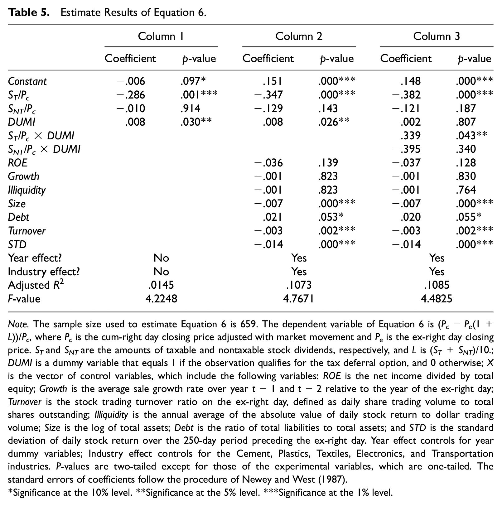
Note. The sample size used to estimate Equation 6 is 659. The dependent variable of Equation 6 is (P_c − P_e(1 +L))/P_c, where P_c is the cum-right day closing price adjusted with market movement and P_e is the ex-right day closing price. S_T and S_NT are the amounts of taxable and nontaxable stock dividends, respectively, and L is (S_T+S_NT)/10.; DUMI is a dummy variable that equals 1 if the observation qualifies for the tax deferral option, and 0 otherwise; X is the vector of control variables, which include the following variables: ROE is the net income divided by total equity; Growth is the average sale growth rate over year t − 1 and t − 2 relative to the year of the ex-right day; Turnover is the stock trading turnover ratio on the ex-right day, defined as daily share trading volume to total shares outstanding; Illiquidity is the annual average of the absolute value of daily stock return to dollar trading volume; Size is the log of total assets; Debt is the ratio of total liabilities to total assets; and STD is the standard deviation of daily stock return over the 250-day period preceding the ex-right day. Year effect controls for year dummy variables; Industry effect controls for the Cement, Plastics, Textiles, Electronics, and Transportation industries. P-values are two-tailed except for those of the experimental variables, which are one-tailed. The standard errors of coefficients follow the procedure of Newey and West (1987).

Significance at the 10% level. **Significance at the 5% level. ***Significance at the 1% level.

Without considering control variables and the interaction terms, Column 1 of Table 5 indicates that the coefficient of S_T/P_c is significant at the 1% level, while that of S_NT/P_c is not significant at any conventional level. Column 2 extends Column 1 by including control variables and year as well as industry fixed effects, and the result does not change, where the coefficient of S_T/P_c remains significant and that of S_NT/P_c remains insignificant. As the most salient difference between S_T and S_NT on the ex-right day is in their tax treatments, these results provide evidence that EPCR in Taiwan reflects the effect of taxes.

Column 3 of Table 5 presents the results from estimating the full specification of Equation 6. As shown in Column 3, the interaction term between S_T/P_c and DUMI is positive and significant, consistent with our hypothesis. This result suggests that the tax deferral option is valuable to investors. The interaction term between S_NT/P_c and DUMI is insignificant; thus, our result reflects the effect of the tax deferral option rather than effects of non-tax firm characteristics related to qualification status for that option.¹⁶ In particular, since the coefficient of S_T/P_c represents investor tax rate, DUMI must capture the effect of the tax deferral option to have a significant effect on investor tax rate.¹⁷

For control variables, the results are largely consistent in both Columns 2 and 3. The coefficient of STD is negative and significant, suggesting that higher idiosyncratic risk is associated with higher stock returns (higher P_e relative to P_c). This is consistent with the finding of Fu (2009) that investors require a higher return as compensation for bearing idiosyncratic risk (Merton, 1987). The coefficient of Turnover is also negative and significant. This suggests that higher trading volume is associated with larger price change (i.e., larger difference between P_e and P_c), consistent with the finding of numerous prior studies (e.g., Karpoff, 1987). Finally, the coefficients of Size and Debt are significant with both negative and positive signs, respectively.

We use Column 3 to evaluate the economic significance of the tax deferral option. Specifically, the coefficient of S_T/P_c is −0.382, which implies that, on average, the tax rate of the marginal investor for taxable stock dividends is 38.2%. The coefficient of S_T/P_c·DUMI is 0.339; thus, with the tax deferral option, investors can reduce their tax rate to 4.3%. This implies a tax deferral parameter of 11.3% (i.e., (0.382 – 0.339/0.382). Furthermore, for a $1 taxable stock dividend, the tax deferral option results in a 33.9¢ tax savings. This result suggests that the tax deferral option benefits primarily investors with high tax rates, especially those with a tax bracket of 40%, since investors in low tax brackets are unlikely to have such high tax savings.

The value of tax deferral is of interest to the finance literature. Miller (1977) assumes that the effective personal tax rate on equity is zero, and partly motivates his assumption by saying that 10-year deferral is equivalent to zero statutory tax. Protopapadakis (1983) estimates the deferral parameter as 25% from actual capital gains taxes paid. Green and Hollifield (2003) report this figure to be 50% to 60% and Chay et al. (2006) suggest that this figure is 55%.

Our estimate of the tax deferral parameter is lower than estimates from prior studies. One possible reason for this is that these studies explore U.S. tax rules, so investors can exercise the restart option. With the restart option, investors may accelerate realization of gains to pay taxes, as suggested by Constantinides (1984). Acceleration of tax payments leads the tax deferral parameter to be higher, and this explains why our estimate is lower. Moreover, because prior studies’ estimates are related to the restart option but ours is not, to some extent, the difference between their estimates and ours reflects the effect of the restart option. Hence, prior studies’ higher tax deferral parameters suggest that investors do exercise the restart option so the restart option is also valuable to them.¹⁸

Out-of-Sample Test

The results of Table 5 support our argument that the tax deferral option is valuable to investors. However, our results may suggest a special case and cannot generalize to a broader population, since observations qualified for the tax deferral option account for a small part of our sample. To address this issue, we conduct an out-of-sample test by analyzing the 798 observations that we exclude from our sample due to the ambiguity of their qualification status.

Tests described in this section involve two-stage analyses. In the first stage, we use DUMI as the dependent variable to run a logistic regression on several explanatory factors with our full sample of 659 observations. We then use the resulting coefficients to estimate the probability of qualifying for the tax deferral option for each of the 798 observations¹⁹ and we set 0.0642 as the cutoff probability²⁰ to determine their qualification status. Based on this cutoff probability, we create a dichotomy variable DUMI_pred that equals 1 for observations with estimated probability higher than 0.0642 and 0 otherwise, where observations with DUMI_pred = 1 are classified as qualifying for the tax deferral option and those with DUMI_pred = 0 are classified as not qualifying. In the second-stage analysis, we re-estimate Equation 6 with the 798 observations and replace DUMI with DUMI_pred.

By assigning each observation an estimated probability, our two-stage procedure expands the measurement of DUMI to all 798 observations; this mitigates the concern that our results based on DUMI are driven by any particular subset of observations. In addition, the cutoff probability 0.0642 leads 283 observations among the 798 observations classified as qualifying for the tax deferral option. This substantially expands the size of observations qualifying for that option, which not only mitigates the concern of small sample size but also helps to evaluate the generalizability of our results. We expect that using DUMI_pred will generate results similar to those using DUMI if our results are not specific to the 59 observations known to qualify for the tax deferral option.

To estimate DUMI_pred, our logistic regression includes the following determinants of qualification status: CAPEX denotes expenditures for equipment investments scaled by total assets; R&D represents research and development expenditures scaled by total assets; INVEST represents expenditures on long-term investments scaled by total assets;²¹MVE is the log of equity market value; REPAY is the repayment of long-term debts scaled by total assets; LTD is long-term debt over total assets; and Growth is defined as in Section “Regression Specification.”

We include R&D and CAPEX because Article 16 of SPIU encourages research and development activities and equipment investments for specific purposes. Therefore, the larger the R&D expenditures or equipment investments a firm makes, the more likely it is to meet the stipulations of Article 16 of SPIU, making it more likely to qualify for the tax deferral option. Similarly, we include INVEST, since Article 16 of SPIU also covers inter-corporate investments in companies within specific industries. INVEST is especially relevant to firms in non-manufacturing industries (e.g., finance or general merchandise), because they typically have very low R&D or equipment expenditures, and their qualification for Article 16 of SPIU depends on their investments in other companies. We include REPAY and LTD because the repayments of loans for purchasing equipment stipulated in Article 16 of SPIU make firms qualify for the tax deferral option and firms typically finance equipment investments with long-term debts. We also include MVE and Growth to control for potential effects of firm size and growth opportunities.

Table 6 shows the results from the two-stage procedure. Panel A of Table 6 presents the results of estimating the logistic regression used to estimate DUMI_pred. Consistent with our expectation, the coefficients of CAPEX, R&D, INVEST, REPAY, and LTD are all positive and significant. Therefore, firms with higher expenditures on equipment investments, R&D activities, inter-corporate investments, or long-term debts are more likely to conform to the stipulations of Article 16 of SPIU.²²

Table 6.

Estimate Results of Out-of-Sample Test With Two-Stage Procedure.

Panel A: logistic regression result			Panel B: estimate result of Equation 6 using DUMIpred
	Column 1			Column 2		Column 3
	Coefficient	p-value		Coefficient	p-value	Coefficient	p-value
Constant	−9.103	.000**	Constant	.096	.000***	.097	.000***
Growth	−1.819	.014**	S_T/P_c	−.281	.003***	−.380	.000***
MVE	0.634	.000***	S_NT/P_c	−.135	.198	−.186	.108
CAPEX	5.268	.000***	DUMI_pred	−.002	.549	−.012	.050**
R&D	0.225	.068*	S_T/P_c × DUMI_pred			.331	.024**
INVEST	3.442	.042**	S_NT/P_c × DUMI_pred			.127	.521
REPAY	7.835	.036**	ROE	−.032	.181	−.032	.185
LTD	2.555	.038**	Growth	−.001	.024**	−.001	.017**
			Illiquidity	.001	.518	.001	.539
			Size	−.006	.000***	−.006	.000***
			Debt	.027	.002***	.026	.003***
			Turnover	−.004	.000***	−.004	.000***
			STD	−.001	.988	.001	.957
			Year effect?	Yes		Yes
			Industry effect?	Yes		Yes
Obs.	659		Obs.	798		798
Pseudo R²	.1036		Adjusted R²	.0873		.0897
			F-value	4.6281		4.4126

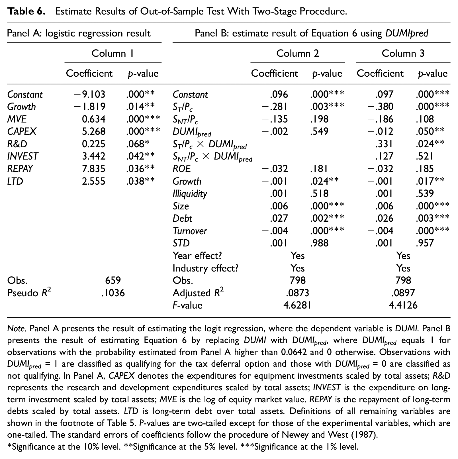
Note. Panel A presents the result of estimating the logit regression, where the dependent variable is DUMI. Panel B presents the result of estimating Equation 6 by replacing DUMI with DUMI_pred, where DUMI_pred equals 1 for observations with the probability estimated from Panel A higher than 0.0642 and 0 otherwise. Observations with DUMI_pred = 1 are classified as qualifying for the tax deferral option and those with DUMI_pred = 0 are classified as not qualifying. In Panel A, CAPEX denotes the expenditures for equipment investments scaled by total assets; R&D represents the research and development expenditures scaled by total assets; INVEST is the expenditure on long-term investment scaled by total assets; MVE is the log of equity market value. REPAY is the repayment of long-term debts scaled by total assets. LTD is long-term debt over total assets. Definitions of all remaining variables are shown in the footnote of Table 5. P-values are two-tailed except for those of the experimental variables, which are one-tailed. The standard errors of coefficients follow the procedure of Newey and West (1987).

Significance at the 10% level. **Significance at the 5% level. ***Significance at the 1% level.

Panel B of Table 6 presents the result of estimating Equation 6 with DUMI_pred. In Column 2 of Table 6, Panel B, the coefficient of S_T/P_c is significantly negative while the coefficient of S_NT/P_c is insignificant, similar to the finding in Table 5. This result rules out the interpretation of non-tax factors on EPCR for the 798 out-of-sample observations.

In Column 3 of Table 6, Panel B, we consider the effect of DUMI_pred on EPCR. The result indicates that the coefficient of S_T/P_c·DUMI_pred is significantly positive and the coefficient of S_NT/P_c·DUMI_pred is insignificant, consistent with our finding in Table 5. In particular, the coefficient of S_T/P_c·DUMI_pred is 0.331, which suggests that the tax deferral option results in a 33.1¢ tax savings for a $1 taxable stock dividend. Together with the coefficient of S_T/P_c−0.380, this result implies a tax deferral parameter of 12.9%, (0.380 – 0.331/0.380). All these inferences are similar to those inferred from Table 5.

Overall, the results in Table 6 corroborate our argument, and this suggests that our conclusion concerning the value of the tax deferral option does not illustrate a special case, but rather, it can generalize to a broader population.²³

Additional Analysis

Trading Volume Around Ex-Right Day

In this section, we investigate how the tax deferral option affects trading volumes around ex-right days. We expect that in contrast to stocks without the tax deferral option, stocks with this option have greater trading volumes around ex-right days. Intuitively, investors prefer tax-favored investment. If they want to invest in firms declaring stock dividends, they will prefer those with the tax deferral option. This suggests that stocks with the tax deferral option have more investors and a larger number of investors naturally implies higher trading volumes. Furthermore, to correspond to our theoretical model of EPCR in Section “Model and Hypothesis Development,” we also provide an analysis as follows that focuses on long-term traders whose only decision around ex-right days is whether to transact before or after the stock goes ex-right.

We first analyze the case of stocks without the tax deferral option. To avoid taxes, buyers will prefer to buy a stock after it goes ex-right because if they buy before going ex-right, they will receive the stock dividends and incur taxes. In contrast, if sellers sell a stock after it goes ex-right, they will receive the stock dividends and incur taxes, so they will prefer to sell before going ex-right. Hence, taxation will induce some buyers to delay their buying decisions to after ex-right days and induce some sellers to accelerate their selling decisions to before ex-right days. The ultimate consequence is that taxation reduces trading volumes on either the cum-right or the ex-right periods. The tax deferral option can mitigate the distortion from taxation because, with this option, buyers have less need to delay their buying decisions and sellers have less need to accelerate their selling decisions.²⁴ We, thus, expect that stocks with the tax deferral option have higher trading volumes either before or after going ex-right than do stocks without that option.

We test our expectation by examining excess share trading volumes. We compute normal trading volume as the annual average of a stock’s turnover ratio minus the annual average of aggregate market turnover ratio (Chay et al., 2006; Michaely & Vila, 1996) measured over the preceding calendar year of the ex-right day. The aggregate market turnover ratio is computed as the aggregate turnover ratio of all stocks listed on Taiwan Stock Exchange. Excess volume on a specific day is a stock’s turnover ratio on that day minus its normal trading volume and that day’s aggregate market turnover ratio. This excess volume measure has the advantage of controlling for both market-wide volume changes and cross-sectional differences in a specific firm’s volume changes.

To explore our argument, we regress excess volumes on DUMI and several explanatory factors that are expected to affect ex-day trading volumes (Michaely & Vila, 1996). Our excess volume measure includes two periods: cum-period excess volume is the average accumulative excess volume over the 3-day cum-right period; similarly, the analog for the ex-period is the average accumulative excess volume over the 3-day ex-right period. Our conclusions remain unchanged if our abnormal trading measure is computed over a 4- or 5-day window. The results for trading volumes are shown in Table 7.

Table 7.

Impact of the Tax Deferral Option on Trading Volume Around Ex-Right Days.

Panel A: estimated with full sample
	Cum-right period result				Ex-right period result
	Column 1		Column 2		Column 3		Column 4
	Coefficient	p-value	Coefficient	p-value	Coefficient	p-value	Coefficient	p-value
Constant	.317	.002***	.351	.454	−.325	.005***	−1.633	.001***
DUMI	.193	.024**	.308	.002***	.305	.005***	.297	.007***
S_T/P_c			−.092	.002***			−.065	.019**
S_NT/P_c			.020	.479			−.037	.248
ROE			−.104	.876			−.212	.735
Growth			.017	.002***			.006	.401
Illiquidity			.003	.447			.005	.151
Size			.003	.913			.092	.001***
Adjusted R²	.061		.075		.062		.072
F-value	4.431		3.866		4.520		3.760
Panel B: estimated with full sample excluding observations declaring only nontaxable stock dividends
	Cum-right period result				Ex-right period result
	Column 5		Column 6		Column 7		Column 8
	Coefficient	p-value	Coefficient	p-value	Coefficient	p-value	Coefficient	p-value
Constant	.284	.015**	−.123	.821	−.243	.065*	−1.681	.008***
DUMI	.304	.002***	.338	.001***	.330	.005***	.352	.005***
S_T/P_c			−.071	.034**			−.100	.013**
S_NT/P_c			.045	.242			−.022	.625
ROE			.240	.774			−1.195	.158
Growth			.014	.000***			.004	.239
Illiquidity			−.003	.847			−.005	.623
Size			.030	.376			.112	.001***
Adjusted R²	.099		.101		.081		.105
F-value	4.839		3.609		4.101		3.763

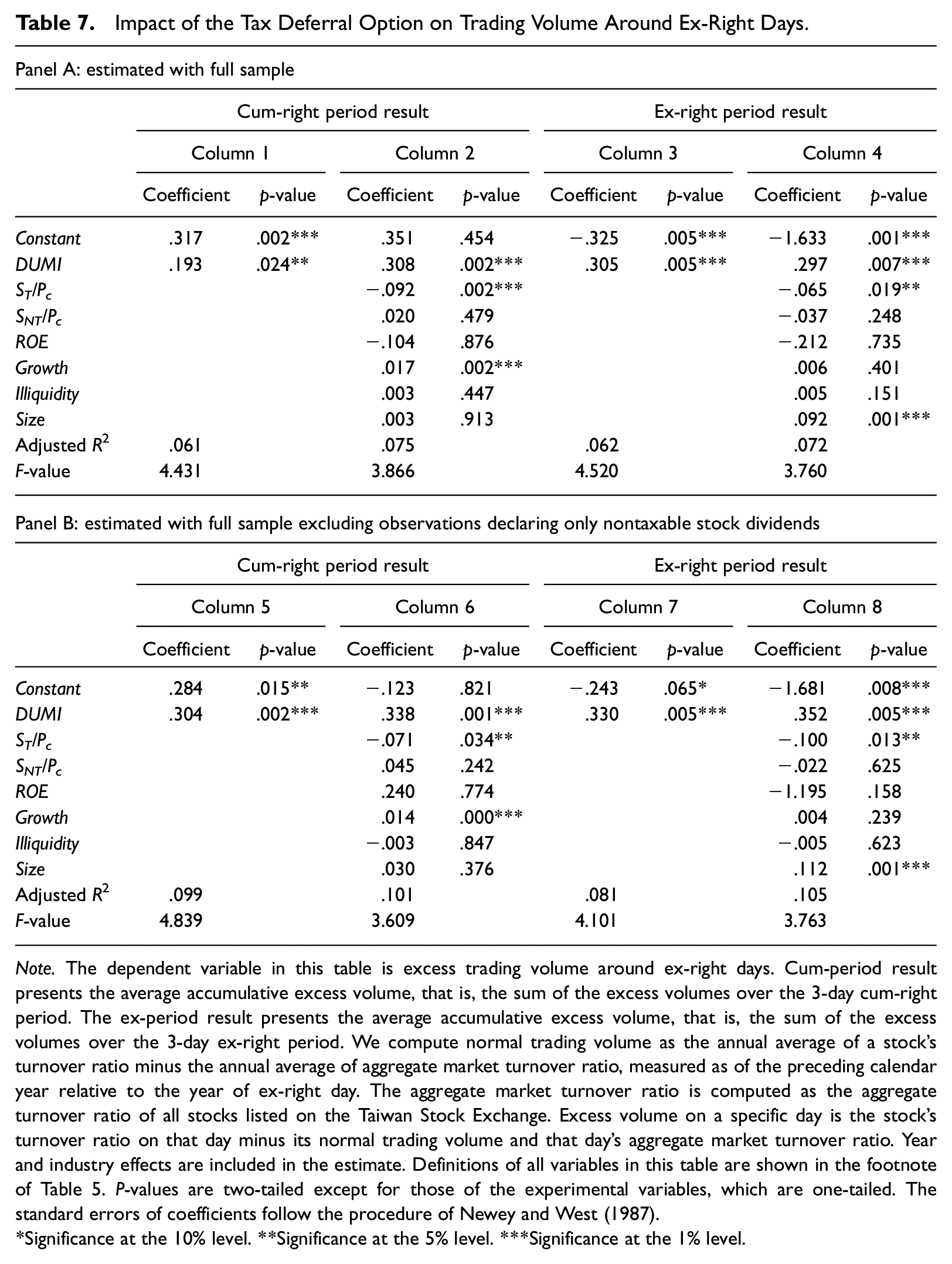
Note. The dependent variable in this table is excess trading volume around ex-right days. Cum-period result presents the average accumulative excess volume, that is, the sum of the excess volumes over the 3-day cum-right period. The ex-period result presents the average accumulative excess volume, that is, the sum of the excess volumes over the 3-day ex-right period. We compute normal trading volume as the annual average of a stock’s turnover ratio minus the annual average of aggregate market turnover ratio, measured as of the preceding calendar year relative to the year of ex-right day. The aggregate market turnover ratio is computed as the aggregate turnover ratio of all stocks listed on the Taiwan Stock Exchange. Excess volume on a specific day is the stock’s turnover ratio on that day minus its normal trading volume and that day’s aggregate market turnover ratio. Year and industry effects are included in the estimate. Definitions of all variables in this table are shown in the footnote of Table 5. P-values are two-tailed except for those of the experimental variables, which are one-tailed. The standard errors of coefficients follow the procedure of Newey and West (1987).

Significance at the 10% level. **Significance at the 5% level. ***Significance at the 1% level.

As shown in Panel A of Table 7, the coefficient of DUMI is positive and significant across all columns, which suggests that stocks with the tax deferral option have greater trading volumes during both the cum-right period and the ex-right period, consistent with our expectation. In Panel B of Table 7, we exclude observations that declare only nontaxable stock dividends because the tax deferral option is not applicable to them. We find that this does not change our findings. Overall, the results in Table 7 confirm that the tax deferral option mitigates the negative impact of dividend taxation on trading volumes around ex-right days. This suggests the role of the tax deferral option in affecting trading behaviors.²⁵

Investor Tax Rate and Value of the Tax Deferral Option

This section explores how investor tax rate affects the value of the tax deferral option. We conduct this test because, despite the apparent advantage of deferring tax payment, there is little evidence to show what factors determine the value of the tax deferral option.

Further discussion for the relation between tax deferral option and EPCR

Under the realization-based taxation rule, investor tax rate is positively associated with the value of tax deferrals. If we let the discounting factor from tax deferral option as 1/(1 + i)ⁿ, where i is the discount rate and n is the period the tax payment is deferred, then EPCR_with can be represented as −t_d multiplied by the discounting factor:

EPC R_{with} = - \frac{t_{d}}{{(1 + i)}^{n}} .

(7)

Equation 7 can be rearranged as follows:

EPC R_{with} = - t_{d} + t_{d} \cdot (1 - \frac{1}{{(1 + i)}^{n}}) .

(8)

Comparing Equation 8 with Equation 4, we know that OP actually equates the term t_d·(1 − 1/(1 + i)ⁿ). This suggests that OP is a function of t_d and a higher t_d leads to a greater OP, while this is a natural relation regardless of i and n. This relation arises because higher tax rate implies greater savings from the present value of tax payment, which in turn implies a higher value of the tax deferral option. This also clarifies why we can view OP as a constant in Equation 4 and subtract it from t_d, since OP will be constant given t_d as constant.

Empirical relation between investor tax rate and the value of the tax deferral option

Discussions in Section “Further Discussion for the Relation between Tax Deferral Option and EPCR” suggest that investor tax rate is a determinant of the value of the tax deferral option. In other words, OP is a function of investor tax rate. We, thus, explore this argument with the interaction term between S_T/P_c·DUMI and a proxy for investor tax rate (WAT in Table 8), given that the coefficient on S_T/P_c·DUMI in Equation 6 (β₄) represents the value of OP so β₄ is a function of WAT. Specifically, β₄ can be represented as follows:

Table 8.

Estimate Result of Equation 6 With Firm-Level Weighted Average Tax Rate of Shareholders.

	Column 1		Column 2		Column 3
	Coefficient	p-value	Coefficient	p-value	Coefficient	p-value
Constant	.113	.000***	.115	.000***	.115	.000***
S_T/P_c	−.357	.000***	−.353	.000***	−.351	.000***
S_NT/P_c	−.039	.674	−.039	.679	−.039	.678
DUMI	.050	.061*	.060	.034**	.060	.049**
S_T/P_c × DUMI	−1.374	.031**	1.536	.033**	−1.477	.028**
S_NT/P_c × DUMI	−1.612	.263	−1.710	.194	−1.566	.230
S_T/P_c × DUMI × WAT	.068	.029**
S_T/P_c × DUMI × TDIS			−.658	.017**
S_T/P_c × DUMI × TFIS					.126	.047**
S_T/P_c × DUMI × LI			−.284	.031**
S_T/P_c × DUMI × HI					.079	.031**
S_NT/P_c × DUMI × WAT	.064	.327	.069	.256	.064	.298
WAT	−.001	.366	−.001	.335	−.001	.340
DUMI × WAT	−.002	.109	−.003	.065*	−.003	.100*
ROE	−.008	.727	−.009	.695	−.009	.696
Growth	−.001	.002***	−.001	.002***	−.001	.002***
Illiquidity	.001	.000***	.001	.000***	.001	.000***
Size	−.006	.004***	−.006	.003***	−.006	.003***
Debt	.002	.872	.003	.773	.003	.777
Turnover	−.003	.003***	−.003	.003***	−.003	.003***
STD	−.011	.004***	−.011	.004***	−.011	.005***
BETA	.009	.243	.009	.240	.009	.250
Year effect?	Yes		Yes		Yes
Industry effect?	Yes		Yes		Yes
Adjusted R²	.142		.142		.142
F-value	4.154		4.043		4.050

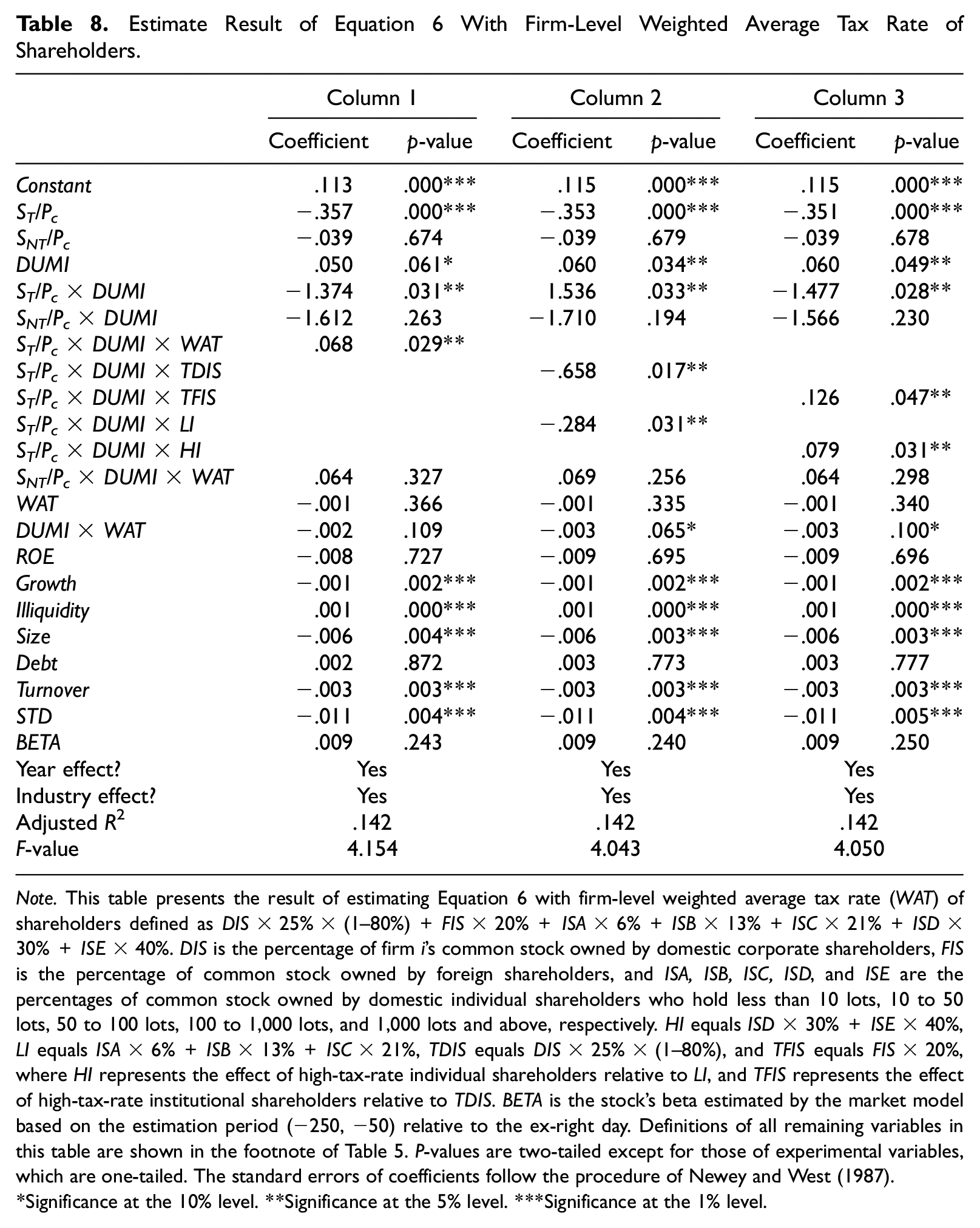
Note. This table presents the result of estimating Equation 6 with firm-level weighted average tax rate (WAT) of shareholders defined as DIS × 25% × (1–80%) + FIS × 20% +ISA × 6% + ISB × 13% + ISC × 21% + ISD × 30% + ISE × 40%. DIS is the percentage of firm i’s common stock owned by domestic corporate shareholders, FIS is the percentage of common stock owned by foreign shareholders, and ISA, ISB, ISC, ISD, and ISE are the percentages of common stock owned by domestic individual shareholders who hold less than 10 lots, 10 to 50 lots, 50 to 100 lots, 100 to 1,000 lots, and 1,000 lots and above, respectively. HI equals ISD × 30% +ISE × 40%, LI equals ISA × 6% + ISB × 13% + ISC × 21%, TDIS equals DIS × 25% × (1–80%), and TFIS equals FIS × 20%, where HI represents the effect of high-tax-rate individual shareholders relative to LI, and TFIS represents the effect of high-tax-rate institutional shareholders relative to TDIS. BETA is the stock’s beta estimated by the market model based on the estimation period (−250, −50) relative to the ex-right day. Definitions of all remaining variables in this table are shown in the footnote of Table 5. P-values are two-tailed except for those of experimental variables, which are one-tailed. The standard errors of coefficients follow the procedure of Newey and West (1987).

Significance at the 10% level. **Significance at the 5% level. ***Significance at the 1% level.

β_{4} = C_{0} + C_{1} \cdot WAT .

(9)

As β₄ reflects the value of OP, C₁ represents the effect of investor tax rate on OP and C₀ represents the effects of determinants other than investor tax rate on OP.

By substituting β₄ in Equation 9, the regression coefficient on S_T/P_c·DUMI in Equation 6 can be rearranged as follows:

\begin{matrix} β_{4} \cdot (\frac{S_{T}}{P_{c}}) \cdot DUMI = (C_{0} + C_{1} \cdot WAT) \cdot (\frac{S_{T}}{P_{c}}) \cdot DUMI \\ = C_{0} \cdot (\frac{S_{T}}{P_{c}}) \cdot DUMI + C_{1} \cdot WAT \cdot (\frac{S_{T}}{P_{c}}) \cdot DUMI . \end{matrix}

(10)

As shown in Equation 10, the coefficient on WAT·S_T/P_c·DUMI is C₁ so we can use it to explore the effect of investor tax rate on OP, where a positive C₁ implies that a higher investor tax rate leads to a greater OP. The coefficient on S_T/P_c·DUMI equates C₀, so it captures any residual effects other than investor tax rate.

We define WAT as firm-level weighted average tax rates of shareholders. We compute WAT through unique ownership data provided by the TEJ database, which includes two kinds of ownership information. One is the proportion of shares held by domestic individual shareholders, foreigners (including both foreign individuals and corporations), or domestic corporate shareholders, and the other is the number of shares held by all shareholders tabulated into lot sizes (one lot is equal to 1,000 shares).²⁶ We estimate the income tax rate of individual investors by calculating their fraction of shareholdings above a particular lot-size threshold. The reasoning is intuitive: as individual shareholders hold more lots, they receive increasing dividend income, leaving them subjected to higher income tax rates under a progressive tax system.

Following Lee et al. (2006), we match average shareholdings in lots to TEJ’s lot-tabulated ranges and define the pairs (effective tax rate range, individual shareholdings based on lot-tabulated ranges) for different tax brackets as: 0%–6%, less than 10; 6%−13%, 10−50; 13%−21%, 50−100; 21%–30%, 100−1,000; and 30%−40%, 1,000 and above.

We separate domestic individual ownership into five variables corresponding to five tax brackets. This allows us to construct WAT as DIS_it × 25% × (1%−80%) + FIS_it × 20% + ISA_it × 6% + ISB_it × 13% + ISC_it × 21% + ISD_it × 30% + ISE_it × 40%. The applicable tax rate depends on the identity of the shareholder group, and DIS_it is the percentage of firm i’s common stock owned by domestic corporate shareholders, FIS_it is the percentage owned by foreign shareholders, and ISA_it, ISB_it, ISC_it, ISD_it, and ISE_it are the percentages owned by domestic individual shareholders who hold less than 10 lots, 10−50, 50−100, 100−1,000, and 1,000 lots and above, respectively.

Based on these data, we extend Equation 6 by incorporating WAT and its interactions with DUMI, S_T/P_c·DUMI, and S_NT/P_c·DUMI.²⁷ The coefficient on S_T/P_c·DUMI·WAT represents C₁ in Equation 10 and we expect it to be positive.

Empirical Results of Incorporating WAT Into Equation 6

Table 8 presents the results of extending Equation 6 by including WAT and its interaction terms.²⁸

As shown in Column 1 of Table 8, the coefficient of S_T/P_c·DUMI·WAT is significant, while the coefficient of S_NT/P_c·DUMI·WAT is insignificant; this rules out non-tax interpretations regarding S_T/P_c·DUMI·WAT. The coefficient of S_T/P_c·DUMI·WAT is .068, suggesting that an increase of one percentage point in the weighted average tax rate (an increase of 1 in WAT)²⁹ produces a 6.8¢ increase in the value of the tax deferral option.³⁰ This result supports our argument that a higher tax rate leads to a higher value of the tax deferral option.

However, using WAT to proxy for investor tax status is subjected to the measurement error that high-tax-rate individuals might actually have low holdings in a specific firm because they are usually wealthier and have more incentives to diversify portfolios. Therefore, stock ownership of individuals who hold low lots might include the ownership of high-tax-rate individuals.

To test whether this measurement error affects our result, we separate WAT into four parts: HI equals ISD × 30% + ISE × 40%, LI equals ISA × 6% + ISB × 13% + ISC × 21%, TDIS equals DIS × 25% × (1%−80%), and TFIS equals FIS × 20%, where HI represents the effect of high-tax-rate individual shareholders relative to LI, and TFIS represents the effect of high-tax-rate institutional shareholders relative to TDIS. We apply this separation to S_T/P_C·DUMI·WAT but not to S_NT/P_C·DUMI·WAT because applying to both cases leads to serious multicollinearity. If high-tax-rate individuals have low holdings, then LI will be confounded by the effect of high-tax-rate individuals and we should find that S_T/P_C·DUMI·LI behaves like S_T/P_C·DUMI·HI.

In Column 2 of Table 8, we first consider the ownership of low-tax-rate shareholders. We find that the coefficients on S_T/P_C·DUMI·LI and S_T/P_C·DUMI·TDIS are both negative and significant. In Column 3 of Table 8, we consider only stock ownership of high-tax-rate shareholders, and the result shows that the coefficients on S_T/P_C·DUMI·HI and S_T/P_C·DUMI·TFIS are both positive and significant. These results suggest that our conjecture that high-tax-rate individuals hold low lots does not lead to serious measurement error of WAT, because S_T/P_C·DUMI·LI behaves differently from S_T/P_C·DUMI·HI.

The coefficient on S_T/P_c·DUMI is negative in Column 1 of Table 8. As shown in Equation 10, incorporating S_T/P_C·DUMI·WAT makes the coefficient on S_T/P_c·DUMI equate C₀, where C₀ reflects the effects of factors other than WAT on the value of OP. As it is unclear about what factors C₀ reflects, it is likely that the coefficient on S_T/P_c·DUMI is negative if C₀ primarily reflects the effects of factors that lead to a lower OP.

The coefficient on S_T/P_c·DUMI is positive in Column 2 but it is negative in Column 3. These results are not contradictory. Specifically, WAT is composed of high- and low-tax-rate stock ownership, denoted as OWN_high and OWN_low, respectively. As Column 3 incorporates the interaction effect between S_T/P_c·DUMI and OWN_high, the coefficient on S_T/P_c·DUMI will include the effect of OWN_low. As the value of the tax deferral option is lower with more low-tax-rate shareholders or a higher OWN_low, it follows that the coefficient on S_T/P_c·DUMI is negative. By similar reasoning, Column 2 incorporates the interaction effect between S_T/P_c·DUMI and OWN_low so its coefficient on S_T/P_c·DUMI includes the effect of OWN_high, suggesting that it is positive. Furthermore, by including only the effect of OWN_high instead of the full effect of WAT, the coefficient on S_T/P_c·DUMI may exceed the upper bound of the tax deferral option (0.4, given the highest tax rate of 40%), which explains why it is so large in Column 2.

Conclusion

We find that the tax deferral option is valuable to investors and this result is not confounded by the restart option. Our study contributes to the literature by providing empirical evidence to estimate the value of the tax deferral option. In particular, we estimate the extent to which investor tax rate affects the value of the tax deferral option; this has been an under-researched, if not unexplored, area.

Some limitations to our results need cautions. First, there are many tax deferral options and we do not attempt to estimate a value that fits all. For example, financial assets other than stocks (e.g., bonds) or real assets (e.g., houses) can also have tax deferral options if their taxation is based on the realization-based rule. As our research design explores stock dividends, the tax deferral option we explore is specific to stock pricing and may not generalize to other tax deferral options. However, this is not a concern because stock pricing is the focus of many finance and accounting studies, particularly given that the effect of tax deferral on equity investments is well recognized but there is little empirical evidence investigating its impacts on stock pricing.

Moreover, not all of our results are applicable to the U.S. tax system because investors’ decisions to defer taxes might be different between Taiwan and the United States due to investor differences in preferences or investment styles. However, one of our main findings is that the tax deferral option is valuable to investors, and we believe that this finding provides guidance for studies exploring the U.S. tax system because this finding results from the realization-based taxation rule, which is the basis of capital gains taxation.

Footnotes

Authors’ Note

Nan-Ting Kuo is now affiliated with Shandong University of Technology, Business School, China.

Declaration of Conflicting Interests

The author(s) declared no potential conflicts of interest with respect to the research, authorship, and/or publication of this article.

Funding

The author(s) received no financial support for the research, authorship, and/or publication of this article.

ORCID iD

Nan-Ting Kuo

Data Availability

Data used in this study are from public sources. A list of sample firms may be obtained from the authors on request.

Notes

References

Amihud

(2002). Illiquidity and stock returns: Cross-section and time-series effects. Journal of Financial Markets, 5, 31-56.

Bali

Hite

G. L.

(1998). Ex-dividend day stock price behavior: Discreteness or tax-induced clienteles? Journal of Financial Economics, 47, 127-159.

Bell

Jenkinson

(2002). New evidence on the impact of dividend taxation and on the identity of the marginal investor. The Journal of Finance, 57, 1321-1346.

Boyd

J. H.

Jagannathan

(1994). Ex-dividend price behavior of common stocks: Fitting some pieces of the puzzle. Review of Financial Studies, 7, 711-741.

Brickley

Manaster

Schallheim

(1991). The tax-timing option and the discounts on closed-end investment companies. Journal of Business, 64, 287-312.

Brown

Clarke

(1993). The ex-dividend day behavior of Australia share prices before and after dividend imputation. Australia Journal of Management, 18, 1-40.

Campbell

Chyz

Dhaliwal

Schwartz

(2013). Did the 2003 Tax Act increase capital investments by corporations? Journal of the American Taxation Association, 35(2), 33-63.

Chay

J. B.

Choi

Pontiff

(2006). Market valuation of tax-timing options: Evidence from capital gains distributions. The Journal of Finance, 61, 837-865.

Cloyd

C. B.

O. Z.

Weaver

C. D.

(2006). Ticks and tax: The effects of price discreteness and taxation on ex-dividend day returns. Journal of the American Taxation Association, 28, 23-46.

10.

Constantinides

G. M.

(1983). Capital market equilibrium with personal tax. Econometrica, 51, 611-636.

11.

Constantinides

G. M.

(1984). Optimal stock trading with personal taxes: Implications for prices and the abnormal January returns. Journal of Financial Economics, 13, 65-89.

12.

Dammon

Dunn

Spatt

(1989). A reexamination of the value of tax options. Review of Financial Studies, 2, 341-372.

13.

Dhaliwal

O. Z.

(2006). Investor tax heterogeneity and ex-dividend day trading volume. The Journal of Finance, 61(1), 463-490.

14.

Ehrhardt

M. C.

Jordan

J. V.

Prisman

E. Z.

(1995). Tests for tax-clientele and tax-option effects in US treasury bonds. Journal of Banking and Finance, 19, 1055-1072.

15.

Elton

E. J.

Gruber

M. J.

(1970). Marginal stockholder tax rates and the clientele effect. Review of Economics and Statistics, 52, 68-74.

16.

Elton

E. J.

Gruber

M. J.

Blake

C. R.

(2005). Marginal shareholder tax effects and ex-dividend-day price behavior: Evidence from taxable versus nontaxable closed-end funds. Review of Economics and Statistics, 87, 579-586.

17.

Francis

J. C.

T. C.

Kuo

N.-T.

(2012). Effects of tax reform on drop-off ratios on the ex-dividend and ex-right prices. Review of Quantitative Finance and Accounting, 39, 147-164.

18.

Frank

Jagannathan

(1998). Why do stock prices drop by less than the value of the dividend? Evidence from a country without taxes. Journal of Financial Economics, 47, 161-188.

19.

(2009). Idiosyncratic risk and the cross-section of expected stock returns. Journal of Financial Economics, 91, 24-37.

20.

Green

R. C.

Hollifield

(2003). The personal-tax advantages of equity. Journal of Financial Economics, 67, 175-216.

21.

Grinblatt

M. S.

Masulis

R. W.

Titman

(1984). The valuation effects of stock splits and stock dividends. Journal of Financial Economics, 13(4), 461-490.

22.

Guenther

D. A.

Sansing

(2010). The effect of tax-exempt investors and risk on stock ownership and expected returns. The Accounting Review, 85, 849-875.

23.

Guo

T. S.

(1996). An investigation on the relationship between the dividend provision and the effective tax rate. [Unpublished thesis]. Department of Finance, National Taiwan University. (In Chinese)

24.

Kalay

(1982). The ex-dividend day behavior of stock prices: A re-examination of the clientele effect. The Journal of Finance, 37, 1059-1070.

25.

Karpoff

(1987). The relation between price changes and trading volume: A survey. Journal of Financial and Quantitative Analysis, 22, 109-125.

26.

Kuo

N. T.

(2012). Dividend tax signaling and the pricing of future earnings: A case of taxable stock dividends. Review of Quantitative Finance and Accounting, 40, 539-570.

27.

Kuo

N. T.

Lee

C. F.

(2013). Effects of dividend tax and signaling on firm valuation: Evidence from taxable stock dividend announcements. Pacific Basin Finance Journal, 25, 157-180.

28.

Lakonishok

Lev

(1987). Stock splits and stock dividends: Why, who, and when. The Journal of Finance, 42(4), 913-932.

29.

Lasfer

M. A.

(2008). Taxes and ex-day returns: Evidence from Germany and the U.K. National Tax Journal, 61, 721-742.

30.

Lee

Y.-T.

Liu

Y.-J.

Roll

Subrahmanyam

(2006). Taxes and dividends clientele: Evidence from trading and ownership structure. Journal of Banking and Finance, 30, 229-246.

31.

O. Z.

Weber

D. P.

(2009). Taxes and ex-dividend day returns: Evidence from REITs. National Tax Journal, 62, 657-676.

32.

McNichols

Dravid

(1990). Stock dividends, stock splits, and signaling. The Journal of Finance, 45(3), 857-879.

33.

Merton

(1987). A simple model of capital market equilibrium with incomplete information. The Journal of Finance, 42, 483-510.

34.

Michaely

(1991). Ex-dividend day stock price behavior: The case of the 1986 Tax Reform Act. The Journal of Finance, 46, 845-860.

35.

Michaely

Vila

(1995). Investors’ heterogeneity, price, and volume around the ex-dividend day. Journal of Financial and Quantitative Analysis, 30, 171-198.

36.

Michaely

Vila

(1996). Trading volume with private valuation: Evidence from the ex-dividend day. Review of Financial Studies, 9, 471-509.

37.

Miller

(1977). Debt and taxes. The Journal of Finance, 32, 261-275.

38.

Naranjo

Nimalendran

Ryngaert

(2000). Time variation of ex-dividend day stock returns and corporate dividend capture: Re-examination. The Journal of Finance, 55, 2357-2372.

39.

Newey

West

(1987). A simple, positive, semi-definite, heteroskedasticity and autocorrelation consistent covariance matrix. Econometrica, 55(3), 703-708.

40.

Pepe

M. S.

(2003). The statistical evaluation of medical tests for classification and prediction. Oxford University Press.

41.

Porter

S. L.

Tse

Yaansah

(2001). The effect of tax rates and transaction costs on the tax trading option: Evidence from stock splits. Journal of Accounting, Auditing, and Finance, 16, 27-53.

42.

Prisman

E. Z.

Roberts

G. S.

Tina

(1996). Optimal bond trading and the tax-timing option in Canada. Journal of Banking and Finance, 20, 1351-1363.

43.

Protopapadakis

(1983). Some indirect evidence on effective capital gains tax rates. Journal of Business, 56(2), 127-138.

44.

Seyhun

H. N.

Skinner

D. J.

(1994). How do taxes affect investors’ stock market realizations? Evidence from tax-return panel data. Journal of Business, 67(2), 231-262.