Relative Effects at Work

NHST

In a case like the order hypothesis in Equation 1, traditional NHST breaks down, as it requires a tremendous number of significance tests that are not necessarily independent or unambiguous. First, four tests are needed for each individual effect, then multiple pairwise comparison tests of the effects need to be conducted to determine if they are significantly different from each other and in the expected direction. Subsequently, it will be very difficult, if not impossible, to combine the resulting set of p values into one single answer to the question of whether the order hypothesis is supported by the data. Also, multiple testing requires type I error corrections (e.g., Bonferroni alpha-correction), which will result in very conservative tests with very little power (Cohen, 1992). Another issue is that there is no straightforward way to understand what the null hypothesis is in this context. For example, do you compare all effects to each other, or only those that are supposed to be closest in magnitude? How do you deal with contradictory results in pairwise comparisons (e.g., β_M is significantly different from β_C, but not from β_P, yet β_C is not significantly different from β_P)? Basically, with order hypotheses or any other moderately complex set of hypotheses, traditional NHST is going to be ineffective. It fails to directly assess the research question of interest.

Traditional model comparison

Instead of NHST, a model comparison approach can be followed as in the popular structural equation modeling (SEM) literature (see, e.g., Bollen, 1989), but even this will not produce definitive assessments of order hypotheses. In such an approach, we start with an a priori set of theoretical models, and then assess and compare these models as a function of the deviation of the sample data from the model and the parsimony of the model. The model that compared to competing models offers an equally good but less complex explanation of the data will be the working model of choice. Balancing fit and parsimony provides guarantees for generalization of the model results to other samples (see, e.g., Hastie, Tibshirani, & Friedman, 2001; Pitt & Myung, 2002). In SEM, model selection is based upon fit statistics (see, e.g., Hu & Bentler, 1999) such as the root mean squared error of approximation (RMSEA) or comparative fit index (CFI), that are formalized according to this “Ockham’s razor” principle. Deviation between data and model is expressed in terms of a Chi-square measure (χ²: summarizing the compatibility of the observed and model-implied covariance matrix) and parsimony is expressed in terms of degrees of freedom (df: the difference between the number of known sufficient sample statistics and the number of unknown model parameters):

Fit = f ( Deviation , Parsimony ) = f ( χ 2 , df ) .

In our example case of workplace aggression, we would tailor the statistical model such that it corresponds as closely as possible to our a priori expectation as formulated in the order hypothesis of Equation 1. Most popular SEM software allow researchers to add the necessary constraints on the model by putting restrictions on the possible values the regression coefficients can take. Hence, an order hypothesis as in Equation 1 can be directly translated into an order-constrained statistical model. If these constraints are quite unreasonable, the constrained model will necessarily show large deviations from the data. If the constraints are consistent with the data, the constrained model will give an approximately equally good yet more parsimonious account of the data patterns than the unconstrained model. Unfortunately, traditional model fit indices are unsuitable for selecting between competing order-constrained models, a point which we will now explain theoretically, but which we will also demonstrate in practice in the first empirical application, the discrimination case (see Table 3, discussed later in this article).

To explain where the incompatibility between traditional fit indices and order hypotheses comes from, let us start with the case of a simple null hypothesis. If we expect aggression from managers and coworkers to have no effect on well-being, we could model this by constraining their effects to be equal to zero. The unconstrained alternative model is obviously less parsimonious than this constrained model, as the former has the flexibility to be consistent with any possible data pattern. The constrained model sets β_M = β_C = 0 and thus has two parameters less, and hence two more degrees of freedom than the unconstrained model. There is a one-to-one correspondence between theoretical precision, model parsimony, and degrees of freedom in the case of equality constraints. In contrast, by imposing the order constraint that the effect of managers is lower in value than the effect of coworkers (i.e., β M < β C ), we do increase the precision of our theory and the informativeness of our hypothesis, but we do not reduce the number of regression coefficients (model parameters), and hence, the degrees of freedom of the constrained model remains exactly the same as those of the unconstrained alternative. Nevertheless, as with equality constraints, order constraints limit the model to a smaller range of potential data patterns, making it more parsimonious and less flexible. Yet simply because the constraints are on the possible parameter values these regression coefficients can take and do not imply a concrete reduction of model parameters, the logic of operationalizing theoretical precision and model parsimony in terms of countable degrees of freedom breaks down. This means that in case of order hypotheses, traditional fit indices reduce to simple deviation measures (see Equation 2) and do not result in a reward for formulating a more focused informative hypothesis. An overly general unconstrained model that fits would be assessed to be equally good as an a priori more risky (i.e., in terms of fit) but more specific and informative order-constrained model. This is highly undesirable if we are to achieve Edwards and Berry’s aim of a strong inference and theoretical precision in management.

Thus, to summarize, both traditional NHST approaches as well as those based on model fit as in SEM are not suitable to test theories and hypotheses involving order constraints. Therefore, we need an alternative approach that is able to test order hypotheses. In the next two sections we will present a Bayesian approach that fits this purpose.

Model Specification: Prior, Likelihood, and Posterior

The design of a research study is typically informed by theory and prior results from the literature. Bayesian data analysis builds upon this starting point by formalizing these prior expectations in terms of probability distributions for the parameters of interest in a statistical model. Hence, such a prior distribution reflects the information we have about the model parameters before observing the data. This can be based on external information sources such as expert judgment and subjective theory, or more empirically based on meta-analysis results of the existing research literature. Another option is to deliberately remain very uncertain and formulate a so-called noninformative (or vague) prior distribution. For the effects of discrimination on well-being, for instance, a uniform prior between an extremely negative and extremely positive value (say between -100 and 100) could be specified. In this case every possible effect across this range is equally likely a priori. This is conceptually similar to taking no theoretical perspective before the analysis starts, and for instance disregarding that the effect will almost certainly be negative. We will denote the prior distribution of the effects β t under model M_t as Pr ( β t | M t ) , where the subscript t simply indicates a number assigned to refer to a specific statistical model or hypothesis (the sign “|” should be read as “conditional on” or “under”).

Having formulated a prior distribution for the parameters of the model, the next step in Bayesian data analysis is to update the prior expectations with the information provided by the collected sample data. This information is formalized in terms of the likelihood which links the data to the statistical model. Note that the likelihood has the same role as in classical statistics. We denote a likelihood by Pr ( data | β t , M t ) , which reads as the probability of the observed sample data under a fixed value β t for the parameter of model M t .

The update, combining information from the prior and from the data, results in the so-called posterior distribution, denoted by “ Pr ( β t | d a t a , M t ) ,” which quantifies the plausibility of the effects β t under model M_t after observing the data. This posterior distribution can be used for traditional forms of estimation and hypothesis testing about parameters (Kruschke, Aguinis, & Joo, 2012): derivation of point estimates (e.g., posterior mode or posterior mean), credibility intervals (i.e., the Bayesian equivalent of confidence intervals), and hypothesis tests for single model parameters or even for nonlinear combinations of model parameters.

Computationally, the underlying updating mechanism that defines Bayesian analysis is based on an application of Bayes’ theorem and often formulated as:

Pr ( β t | d a t a , M t ) ∝ ︸ P o s t e r i o r Pr ( β t | M t ) × ︸ P r i o r Pr ( d a t a | β t , M t ) ︸ L i k e l i h o o d ,

where Equation 3 reads as “posterior is proportional to prior times likelihood.”

In contrast to a Bayesian approach, a classical frequentist data analysis approach would seek to find the point estimate for the parameter, denoted by β ∧ t , for which the likelihood is maximized. Prior distributions are not used in a frequentist analysis, and hence one is always in an uninformed prior setting and only informed by the data. The downside is that one only has a single value for the model parameters and not the broader probability information available in a Bayesian approach. Yet for some the frequentist approach still sounds like a more objective and less controversial approach than a Bayesian data analysis with priors. However, the actual impact of a prior distribution decreases proportionally with increasing sample size (i.e., the data will dominate the prior) and a Bayesian approach can always mimic a frequentist analysis by using noninformative priors.

The reverse cannot be said; often for complex hypothesis tests or more complex statistical models, no straightforward frequentist solution exists, when a Bayesian approach can offer a viable solution. Where a frequentist approach fails, the smart use of priors in a Bayesian approach will allow us to construct a proper tool for model comparison among competing models that reflect different order hypotheses. For this reason, one should not think of prior specification as an Achilles’ heel of Bayesian statistics. Instead, priors and Bayesian data analysis in general provide researchers with a very flexible and broadly applicable informative approach to statistical inference.

Model Comparison: Marginal Likelihoods and Bayes Factors

Above we introduced the idea of Bayesian data analysis and estimation, where prior expectations are updated by the likelihood, a mechanism that was summarized in Equation 3. The exact version of the Bayes Theorem, given in Equation 4 below,

Pr ( β t | data , M t ) ︸ P o s t e r i o r = Pr ( β t | M t ) ︷ P r i o r × Pr ( data | β t , M t ) ︷ L i k e l i h o o d Pr ( data | M t ) ︸ M a r g i n a l l i k e l i h o o d

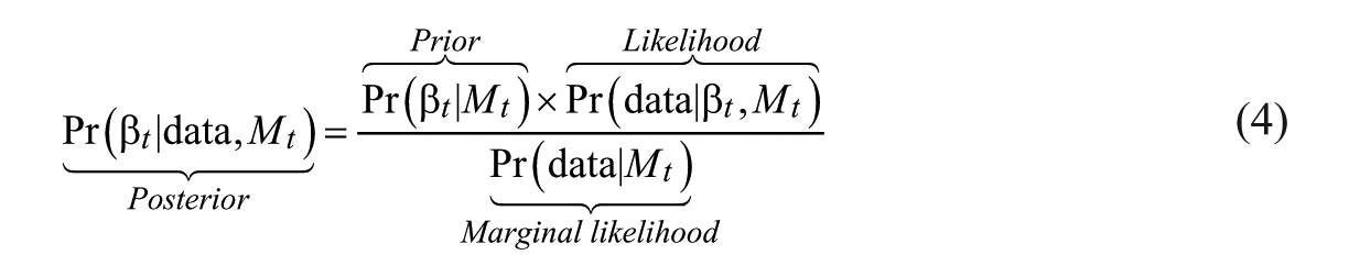
includes yet another term that is commonly referred to as the marginal likelihood, denoted by Pr ( data | M t ) . This term can be omitted in estimation procedures because it is a normalizing constant that does not affect general Bayesian estimation techniques and is only theoretically necessary to make the posterior a “proper” probability distribution (i.e., with total probability summing to 1). However, for model comparison purposes, this marginal likelihood is a very informative measure.

Formally the marginal likelihood of a model M_t, Pr ( data | M t ) , is the expected probability of the data across the whole range of values of the prior distribution of the model parameters. In essence, the marginal likelihood computes an average level of fit to the data for a model M_t and summarizes the amount of evidence in the data for model M_t. More complex models that correspond to less specific theories can fit many different data patterns by changing their parameter values, but will have lower average levels of fit than simpler models that can fit a more limited set of data patterns and correspond to more specific theories (see, e.g., Lodewyckx et al., 2011). Raftery (1993) argues that the marginal likelihood is the optimal criterion for model comparison, as it incorporates and balances both model fit as well as model parsimony.

The Bayes factor is a Bayesian model comparison criterion that builds upon this balancing property of the marginal likelihood and quantifies the relative evidence between two scientific theories or hypotheses (Jeffreys, 1961; Kass & Raftery, 1995). The Bayes factor between two models, say M₁ and M₂, is defined as the ratio of the marginal likelihoods of the two models:

BF ( M 1 , M 2 ) = Pr ( data | M 1 ) Pr ( data | M 2 ) .

In contrast to traditional fit indices, a Bayes factor is interpretable without recourse to qualifiers or commonly accepted thresholds (such as a significance level of .05). For instance, when the Bayes factor is larger than 1, say, BF ( M 1 , M 2 ) = 10 , there is simply 10 times more evidence in the data for model M₁ than for M₂. When the Bayes factor is smaller than 1, say BF ( M 1 , M 2 ) = 0 . 10 , model M₁ receives 10 times less evidence from the data than M₂. Because marginal likelihoods balance model fit and parsimony, the Bayes factor will favor the simpler explanation (i.e., model or hypothesis) that does adequately fit the data. Bayes factors have some convenient properties that add to an easy and consistent interpretation of supporting evidence in the data for the models that are being compared. Reversing the roles of the two models simply leads to reversing the Bayes factor: BF ( M 1 , M 2 ) = 1 / BF ( M 2 , M 1 ) ; or in other words, if there is four times more evidence in the data for model M₁ than for model M₂, this logically implies that there is four times less evidence in the data for model M₂ than for model M₁. Bayes factors between different models can also be indirectly linked, as long as they have a common referent using the transitivity property. For instance, if BF ( M 1 , M 2 ) = 4 and BF ( M 3 , M 2 ) = 8 , then BF ( M 3 , M 1 ) = 8 / 4 = 2 ; or in other words, if model M₁ and M₃ have, respectively, four and eight times more evidence than model M₂, then this implies that model M₃ has two times more evidence than model M₁.

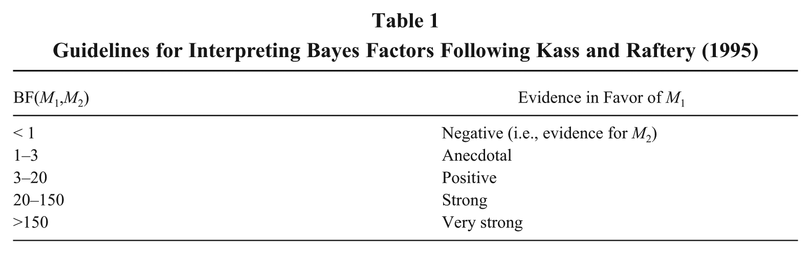
As with effect sizes (Cohen, 1992), tentative guidelines have been provided on how to interpret the outcome of the Bayes factor in a more absolute sense. Table 1 shows the interpretation as proposed by Kass and Raftery (1995). These guidelines can be used as a convenient default starting point for interpreting Bayes factors. Hence, researchers can make statements such as there is “positive” or “very strong” evidence in the data for a certain model against another model based on the observed Bayes factor.

OPEN IN VIEWER

Table 1

Guidelines for Interpreting Bayes Factors Following Kass and Raftery (1995)

BF(M1,M2)	Evidence in Favor of M1
< 1	Negative (i.e., evidence for M2)
1–3	Anecdotal
3–20	Positive
20–150	Strong
>150	Very strong

An Encompassing Model Approach to Bayes Factors

Making use of the proportionality of order-constrained models to an unconstrained model, the computation of Bayes factors for order hypotheses can avoid complicated integration problems. The only requirement is that an encompassing unconstrained model exists, which is the more general version of the order-constrained model(s) so that all models are nested within the encompassing model. The shortcut computation then comes down to determining the Bayes factor between a constrained model M_t and the unconstrained model M_u as the posterior probability that the order constraints hold under the unconstrained model (i.e., f_t a measure of fit for M_t) weighted by the prior probability that the order constraints hold under the unconstrained model (i.e., c_t a measure of complexity for M_t) (for the technical derivation of this shortcut, see the Appendix):

BF ( M t , M u ) = f t c t .

We will first discuss the two elements in the ratio of Equation 6, prior complexity and posterior fit, and then show how the combination of both yields a Bayes factor that can quantify the evidence in the data for an order hypothesis and in turn facilitates straightforward comparisons between different order hypotheses. For the latter purpose, we will show how the concept of posterior model probability enables clear and easy interpretation of the model comparison results.

Prior complexity

Figure 1 illustrates the proportionality idea for the prior distributions and the complexity term c_t. Each model in the working example is represented in a bidimensional plot where the x-axis represents the possible values the effect of aggression from coworkers β C can be expected to take a priori under the unconstrained model, and where the y-axis has a similar function but for the effect of aggression from managers β M . This bidimensional plot is the graphical representation of the prior distribution of β M and β C under the unconstrained model. The gray areas represent the combination of values of β M and β C that satisfy the constraints of each individual model. The complexity of the unconstrained model is for instance equal to 1 as all values for β M and β C are possible, which means that the whole area is covered (Figure 1, lower right panel). For Model 1 (Figure 1, upper left panel), only positive values of β M and β C are possible, constraining the area to the upper-right quadrant that takes up one fourth of the space compared to the unconstrained model. The complexity of Model 1 is therefore equal to one fourth, less complex than the unconstrained model and only compatible with a limited set of possible results. In a similar fashion, for Model 2 (Figure 1, upper right panel) only half of the area is consistent with the constraint that β M > β C , and its complexity is consequently equal to a half. Because M₃ is a combination of M₁ and M₂, the constrained area of M₃ is equal to the area where the constrained areas of M₁ and M₂ overlap, which comes down to a complexity of one eighth (Figure 1, lower left panel). The model that corresponds to the most informative hypothesis/precise theory results in the most specific constrained area and the lowest complexity measure.

OPEN IN VIEWER

Figure 1

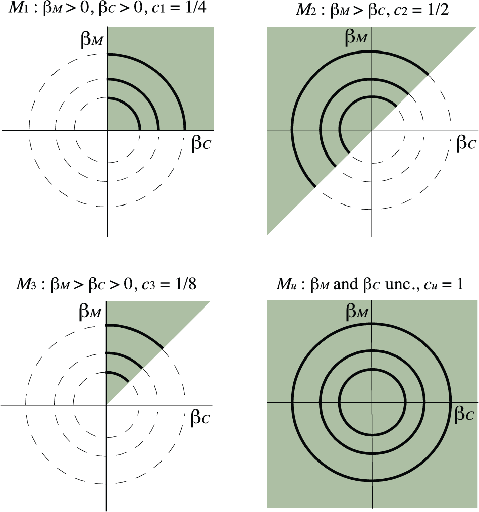
Prior Complexity c_t of Order-Constrained Models

Posterior fit

To illustrate the proportionality idea for the posterior distribution and the fit term f_t, we will consider two hypothetical data sets under the same set of models: Data A with maximum likelihood estimates β ^ M = 0 . 8 and β ^ C = 0 . 3 and Data B with maximum likelihood estimates β ^ M = 0 . 3 and β ^ C = 0 . 8 (both under the unconstrained model). Figure 2 locates the posterior distribution of β_M and β_C under the unconstrained model for Data A and Data B as smaller inner circles in the same plots as we used for the prior distributions. The fit measure in use is a direct reflection of the extent to which the posterior distributions fall into the area of the unconstrained prior distribution that is consistent with the order constraints of the model. For Data A, for instance, we can conclude that the posterior falls completely within the area with possible values that are consistent with the constraints within each model. This implies that the fit of all order-constrained models is maximal and that the model fit terms are all equal to 1. For Data B, we conclude that model M₁ shows maximal fit equal to 1, but that models M₂ and M₃ show complete misfit with a fit measure equal to zero because the posterior distribution does not overlap with the a priori possible area.

OPEN IN VIEWER

Figure 2

Posterior Fit f_t for Data A and Data B of Order-Constrained Models

Bayes factor

Balancing the complexity and the fit measure as in Equation 6 then leads to the Bayes factor (i.e., BF ( M t , M u ) = f_t / c_t). As under Ockham’s razor, when models equally fit the data (which is the case for Data A, see Table 2), the least complex model (i.e., M₃) is preferred—in this case, with the Bayes factor indicating that, compared to the unconstrained model M_u, there is eight times more evidence in the data for model M₃, which is two times more than for M₂ and four times more than for model M₁. For Data B we can see that there is four, zero, and zero times more evidence for M₁, M₂, and M₃, respectively, than for the unconstrained model M_u. Hence, based on these Bayes factors, models M₂ and M₃ receive no support at all from the data. This also makes sense because the order constraints are not supported by the maximum likelihood estimates based on Data B.

OPEN IN VIEWER

Table 2

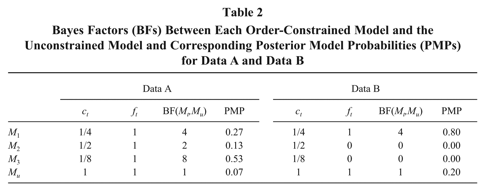
Bayes Factors (BFs) Between Each Order-Constrained Model and the Unconstrained Model and Corresponding Posterior Model Probabilities (PMPs) for Data A and Data B

	Data A					Data B
	ct	ft	BF(Mt,Mu)	PMP		ct	ft	BF(Mt,Mu)	PMP
M 1	1/4	1	4	0.27		1/4	1	4	0.80
M 2	1/2	1	2	0.13		1/2	0	0	0.00
M 3	1/8	1	8	0.53		1/8	0	0	0.00
Mu	1	1	1	0.07		1	1	1	0.20

Bayes Factors and Posterior Model Probabilities

In this section, we will connect the Bayes factor to what is called posterior model probability. The latter will be useful for interpretation of the results of comparisons between multiple models, but also for illustrating that Bayes factors are not affected by common misconceptions that haunt frequentist hypothesis testing and p values.

Similar to the mechanism that we described to update the prior with the likelihood to obtain the posterior, the Bayes factor can be used to update the prior model odds to obtain the posterior model odds according to:

Pr ( M 1 | data ) Pr ( M 2 | data ) ︸ P o s t e r i o r m o d e l o d d s = BF ( M 1 , M 2 ) ︸ B a y e s f a c t o r × Pr ( M 1 ) Pr ( M 2 ) ︸ P r i o r m o d e l o d d s .

In Equation 7, Pr(M_t) denotes the prior model probability of M_t, which is the probability that model M_t is true before observing the data, and Pr(M_t | data) denotes the posterior model probability of M_t, the probability that model M_t is true after observing the data. Note that the prior model probability Pr(M_t) is different from the prior distribution Pr ( β t | M t ) : the first specifies how likely model M_t is before observing the data, while the latter specifies how large the effects β t (i.e., model parameters) are expected to be under model M_t a priori. Because in practice prior model probabilities are often chosen to be equal (i.e., Pr(M₁) = Pr(M₂)), the prior model odds in Equation 7 reduce to 1 and the posterior odds are then simply equal to the Bayes factor.

Posterior odds for a set of models can be transformed into a set of posterior model probability for these models. Consider the four models in our working example, assuming equal prior model probabilities of Pr ( M 1 ) = Pr ( M 2 ) = Pr ( M 3 ) = Pr ( M u ) = 1 / 4 we can use the Bayes factors of all models against the same benchmark model to compute a set of posterior model probabilities. The posterior model probability of a model M_t can be obtained as a normalized weight:

Pr ( M t | data ) = BF ( M t , M u ) BF ( M 1 , M u ) + BF ( M 2 , M u ) + BF ( M 3 , M u ) + BF ( M u , M u ) ,

(i.e., a proportion computed as the Bayes factor of one model in the set against the reference model divided by the sum of Bayes factors of all models in the set against the same reference). The resulting posterior model probabilities for Data A and Data B can be found in Table 2. For Data A, model M₃ has the largest posterior model probability of 0.53, followed by gradual decrease over M₁ and M₂, towards M_u, and for Data B, model M₁ has clearly the largest posterior model probability of 0.80, followed by M_u, whereas models M₂ and M₃ result in posterior model probabilities of zero. Posterior model probabilities always will sum up to 1 within a set, offering a convenient frame of reference for the relative magnitude of a posterior probability. In our experience researchers find that this reference frame makes posterior model probabilities easier to interpret compared to Bayes factors, where they might need to rely on guidelines with which they are not familiar. The risk is, of course, that people might be inclined to request fixed cut-off values for posterior model probabilities in a similar fashion to the widely used 0.05 p value threshold in the case of NHST. But the Bayes factors and posterior model probabilities are best used as relative measures of evidence between two or more models, and they avoid some of the pitfalls of the traditional p values.

With the concept of posterior model probability we can understand better some misconceptions that surround classical p values. In fact classical p values are often misinterpreted as being the (posterior model) probability that a null model is true, but a p value is only equal to the probability of observing more extreme data than the observed data under the condition that the null hypothesis is true. As shown by Sellke, Bayarri, and Berger (2001), the misinterpretation of the p value as a posterior model probability results in serious overestimation of the evidence against the null model. Under very reasonable assumptions (such as equal prior model probabilities), a p value of 0.05 results in a posterior model probability that the null model is true of 0.29, showing how p values underestimate evidence in favor of null hypotheses. Furthermore, whereas we might be inclined to assume that a significant model M 1 with p < 0.01 is 10 times more supported than a significant model M 2 with p < 0.001, we would be making a serious error of judgment and confuse p values with error probabilities (Hubbard & Armstrong, 2006). In contrast, the ratio of two posterior model probabilities 0.01 versus 0.001 (computed among the same set of models) is simply equal to the corresponding Bayes factor BF ( M 1 , M 2 ) = 0.01/0.001 = 10. These discrepancies illustrate that researchers should be very careful when interpreting p values as measures of evidence for model selection and hypothesis testing, and that posterior model probabilities and Bayes factors are to be preferred over classical p values because of their more intuitive interpretation.

Details on Prior Specification

This subsection will deal with the practical implementation of our approach. The contents will therefore be particularly useful for readers who are more familiar with the technical aspects of statistical modeling.

Software Package BIEMS

BIEMS (Bayesian inequality and equality constrained model selection; Mulder et al., 2012) is a freely downloadable software package (www.jorismulder.com) with a user-friendly interface that implements the proposed Bayesian approach to hypothesis testing and model comparison. The two unique aspects of BIEMS are the automatically generated CECPP prior distribution, which ensures no prior preference towards a certain ordering of the effects, and the efficient computation of Bayes factors through the balancing of model fit f_t and model complexity c_t.

To use BIEMS, first, the data must be uploaded and the number of outcome variables and predictors must be specified. Second, the models must be specified with order constraints and equality constraints. Third, the automatic CECPP prior is constructed. In the fourth optional step, one could view and if necessary alter the prior (e.g., when a priori knowledge is available). In the fifth and final step, Bayes factors of each constrained model against the unconstrained model and other model diagnostics are reported. A user manual can be found in Mulder et al. (2012). An accessible tutorial paper about the use of BIEMS is provided by Kluytmans, van de Schoot, Mulder, and Hoijtink (2012).

Despite the effectiveness of Bayesian data analysis, Bayesian methods have not been implemented in many commercial statistical packages, and for now, Bayesian testing of order-constrained models has not yet been implemented elsewhere. Recent developments in Mplus show some promise for the future as the development team decided to implement Bayesian estimation methods because of their superiority over frequentist methods in the case of small samples and its flexibility in fitting complex models using Markov chain Monte Carlo (MCMC) techniques (Muthén & Asparouhov, 2012). The latest version of Mplus supports a very broad Bayesian estimation approach, but unfortunately a formulation of the necessary CECCP priors is not yet possible. We expect that future versions will allow the user to have more control over the priors enabling the method proposed here. For the time being, van de Schoot, Hoijtink, Hallquist, and Boelen (2012) have suggested a very rudimentary pragmatic approach by manually computing the model fit term f_t as the proportion of posterior simulations under the unconstrained model that are in line with the order hypothesis and approximating the model complexity term c _t by means of a proportion based upon the number of possible rank orderings (permutations) among predictors. This might be a little bit too involved for regular use, and it is difficult to apply it to hypotheses with many order constraints.

The following section illustrates our approach in practice and discusses two empirical examples from organizational research where BIEMS was effectively used to determine which of a set of scientific theories receives most evidence from the data.

Application 1: Workplace Discrimination From Inside and Outside the Organization

In the first example we assess competing hypotheses on the effect of perceived discrimination from different sources inside and outside the organization. Considerable evidence exists on detrimental psychological and health effects of experiencing discrimination at work (Goldman, Gutek, Stein, & Lewis, 2006). Perceived workplace discrimination is operationalized by means of single-item measures that capture individuals’ own summary terms they use to reflect their feelings (Wood, Stride, & Johnson, 2012: 538). It captures people’s perceptions of whether they have been discriminated against, as opposed to imposing a label, which victims might not agree with based on various behaviors that may or may not have been interpreted in an adverse manner. Because the study was aimed at a broad range of issues and not all issues could be covered in-depth, the use of single-item measures also reflected the practical constraints for the study with respect to survey length and cognitive load. Respondents simply indicated whether they experienced any form of discrimination in the past 12 months with reference to each of the following potential sources: managers, coworkers, patients, and visitors. Thus, we have instances of workplace discrimination from four different sources inside and outside the organization.

Model 1: Negative impact (M₁)

The first model is rather unspecific and only makes the assumption that perceived discrimination decreases a worker’s well-being regardless of the source. Given that our well-being outcomes are all negatively formulated—anxiety, depression, job dissatisfaction—we expect all regression coefficients of the discrimination sources to be positive (i.e., discrimination implies more anxiety). This constrained hypothesis is formulated as:

M 1 : ( β M , β C , β P , β V ) > 0 ⇔ { β M > 0 β C > 0 β P > 0 β V > 0 ,

where we denote after the left curly bracket the separate restrictions that need to be specified in the BIEMS software to construct this model. Table 3 provides the order constraints of this model, and its competitor models below, as implemented in BIEMS.

OPEN IN VIEWER

Table 3

Order-Constrained Models as Implemented in BIEMS for Application 1

Model	Order Constraints in BIEMS
M 1 (negative impact):	α ( 1 , 1 ) > 0 , α ( 2 , 1 ) > 0 , α ( 3 , 1 ) > 0 , α ( 4 , 1 ) > 0
M 2 (power diff.):	α ( 1 , 1 ) > α ( 2 , 1 ) , α ( 1 , 1 ) > α ( 3 , 1 ) , α ( 2 , 1 ) > α ( 4 , 1 ) , α ( 3 , 1 ) > 0 , α ( 4 , 1 ) , α ( 4 , 1 ) > 0
M 4 (con. sov.):	α ( 1 , 1 ) > α ( 3 , 1 ) , α ( 3 , 1 ) > α ( 2 , 1 ) , α ( 3 , 1 ) > α ( 4 , 1 ) , α ( 2 , 1 ) > 0 , α ( 4 , 1 ) > 0
M 4 (social contact:	α ( 2 , 1 ) > α ( 1 , 1 ) , α ( 2 , 1 ) > α ( 4 , 1 ) , α ( 3 , 1 ) > α ( 1 , 1 ) , α ( 3 , 1 ) > α ( 4 , 1 ) , α ( 1 , 1 ) > 0 , α ( 4 , 1 ) > 0

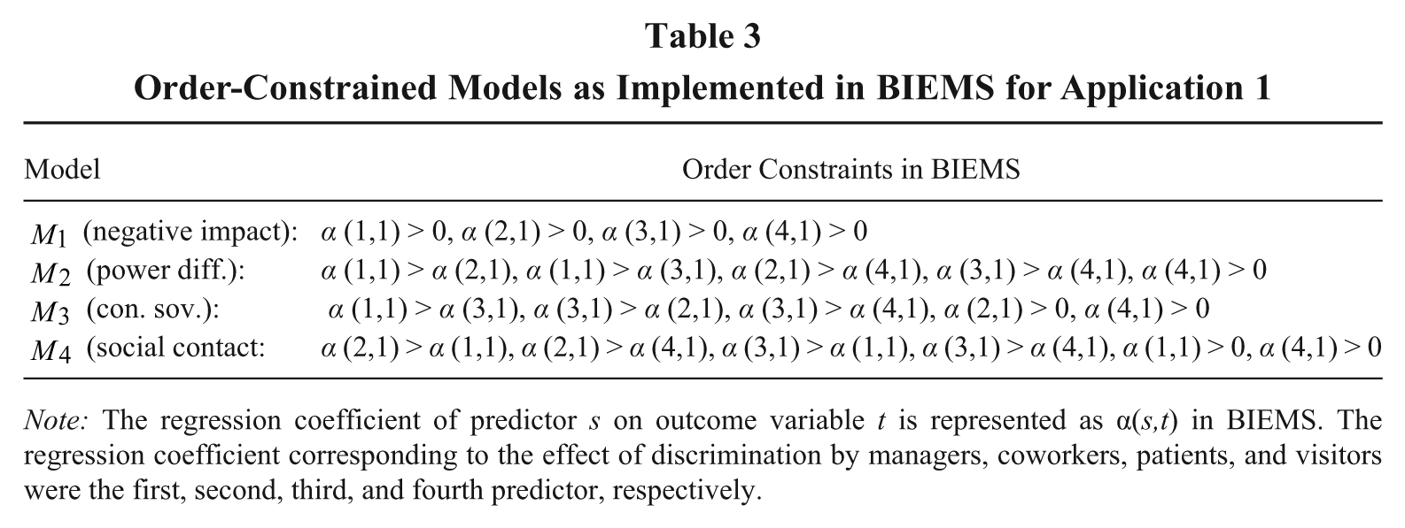
Note: The regression coefficient of predictor s on outcome variable t is represented as α(s,t) in BIEMS. The regression coefficient corresponding to the effect of discrimination by managers, coworkers, patients, and visitors were the first, second, third, and fourth predictor, respectively.

Model 2: Power differential (M₂)

The second model builds on the insider-outsider theory of the effects of workplace aggression introduced earlier (Hershcovis & Barling, 2010), according to which the effects of discrimination from insiders, because they are assumed to have more power over victims than do outsiders, will have more effect on victims’ well-being. Elaborating on this power-differential hypothesis, we expect that discrimination from one’s manager will have the largest impact on the employee. In line with this reasoning, we assume that workplace discrimination by visitors has the least negative effect, because visitors are outsiders entering the organization’s premises. Within the settings of a mental health organization, the middle ground is expected to be covered by coworkers and patients. Coworkers are insiders who may have high expertise and referent power, the latter being particularly important as it is likely “to affect the presence and quality of social relationships within the group” (Hershcovis & Barling, 2010: 28). The patients are outsiders, but do have some power over staff and are both subject to organizational policies and users of organizational policies. This order hypothesis is formulated as:

M 2 : β M > ( β C , β P ) > β V > 0 ⇔ { β M > β C β M > β P β C > β V β P > β V β V > 0 .

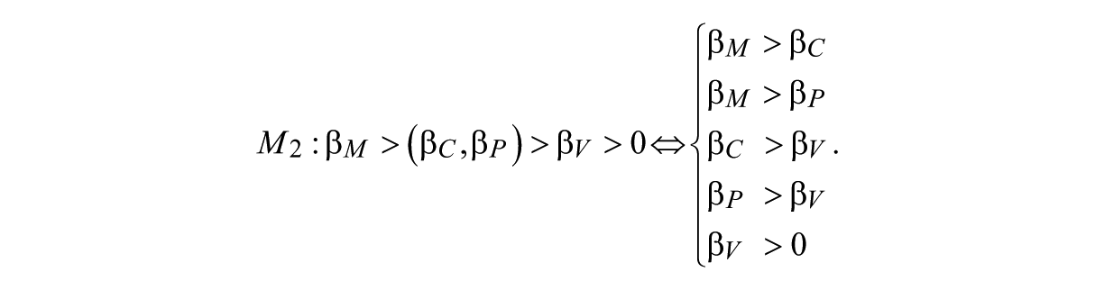
We again operate under the expectation that workplace discrimination, regardless of the source, is detrimental to the victim’s well-being (i.e., corresponding to Model 1). The part ( β C , β P ) indicates that we do not specify an ordering between these two coefficients. After the left curly bracket we show the separate restrictions that need to be specified in the BIEMS software to construct this model (see Table 3). It is not necessary to add, say, β M > β V , because this constraint is a direct logical consequence of β M > β C and β C > β V , which are already specified.

Model 3: Consumer sovereignty and patient’s rights (M₃)

The third model acknowledges the primary position of the manager, but posits the patients as the second most impactful source of discrimination, having a greater effect than that of colleagues or visitors. An argument might be made that notions such as customer sovereignty and citizens/patients rights place an onus on representatives of organizations to treat customers, clients, and patients “with courtesy and as if they are right” (Grandey, Kern, & Frone, 2007: 65) even if those people are acting inappropriately. Thus, the customer, client, or patient is ordained with some degree of legitimate power. Moreover, patients and other outsiders, like customers (Gettman & Gelfand, 2007), also have some power to reward or punish staff, and how staff relates to patients is increasingly given prominence in appraisal and reward systems. Furthermore, in situations where the perpetrator can develop a more enduring relationship with the organization, as is the case with a patient who has a long hospital stay, referent power can be developed. As such, patients may have greater power compared with work colleagues, as well as visitors. Maintaining the assumption that all sources have an effect (see Model 1), this order hypothesis is then formulated as:

M 3 : β M > β P > ( β C , β V ) > 0 ⇔ { β M > β P β P > β C β P > β V β C > 0 β V > 0 .

Model 4: Social contact (M₄)

The fourth hypothesis is based on the idea that the intensity of social contact with the different sources might be the key explanation behind their impact on a worker’s well-being. Given that mental health workers in general have more frequent face-to-face contact with both colleagues and patients, discrimination from them can be hypothesized to have more impact on victim’s well-being than that from managers or visitors. This order hypothesis is then formulated as:

M 4 : ( β C , β P ) > ( β M , β V ) > 0 ⇔ { β C > β M β C > β V β P > β M β P > β M β M ​ > 0 β V > 0 .

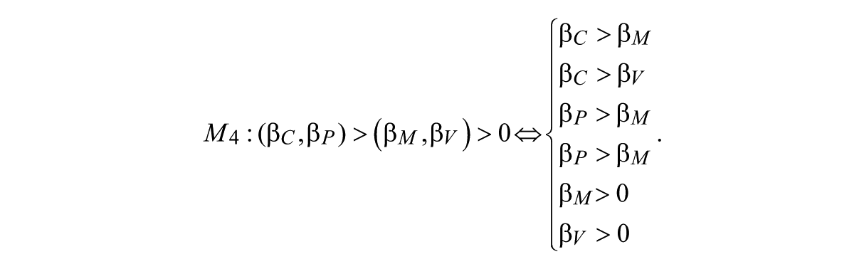
We again operate under the expectation that workplace discrimination, regardless of the source, is detrimental to the victim’s well-being (i.e., corresponding to Model 1).

Model comparison

Bayes factors were computed for each of the four constrained models against the unconstrained model, using BIEMS. The results for the three outcomes—anxiety, depression, and job dissatisfaction—can be found in the upper panel of Table 4, together with the resulting posterior model probabilities and values for a popular traditional fit index, the Comparative Fit Index (CFI). In the lower panel of Table 4, the 95% credibility intervals of the regression coefficients are represented for the unconstrained model.

OPEN IN VIEWER

Table 4

Bayes Factors (BF) for the Constrained Models (M_t) Versus the Unconstrained Model (M_u), Posterior Model Probabilities (PMP), and 95% Credibility Intervals of the Regression Coefficients of the Effects of the Four Sources of Discrimination, Derived for Each Outcome Variable Separately

Model/Outcome	Model Comparison Results
	Anxiety			Depression			Job Dissatisfaction
	BF(Mt, Mu)	PMP	CFI	BF(Mt, Mu)	PMP	CFI	BF(Mt, Mu)	PMP	CFI
Mu	1.0	0.01	1	1.0	0.01	1	1.0	0.00	1
M1 (negative impact)	14.7	0.08	1	15.9	0.16	1	12.3	0.06	1
M2 (power diff.)	68.6	0.39	1	68.0	0.69	0.99	110.8	0.50	1
M3 (con. sov.)	91.9	0.52	1	13.8	0.14	0.99	96.6	0.44	1
M4 (social contact)	0.0	0.00	0.85	0.0	0.00	0.86	0.0	0.00	0.88
	95% Credibility Intervals for the β Effects Under Mu
Predictors/Outcome	Anxiety			Depression			Job Dissatisfaction
Managers	[0.47, 0.80]			[0.54, 0.86]			[0.56, 0.89]
Coworkers	[0.01, 0.33]			[0.17, 0.49]			[0.06, 0.37]
Patients	[0.08, 0.41]			[0.01, 0.32]			[0.13, 0.45]
Visitors	[-0.06, 0.39]			[-0.00, 0.44]			[-0.14, 0.30]

a

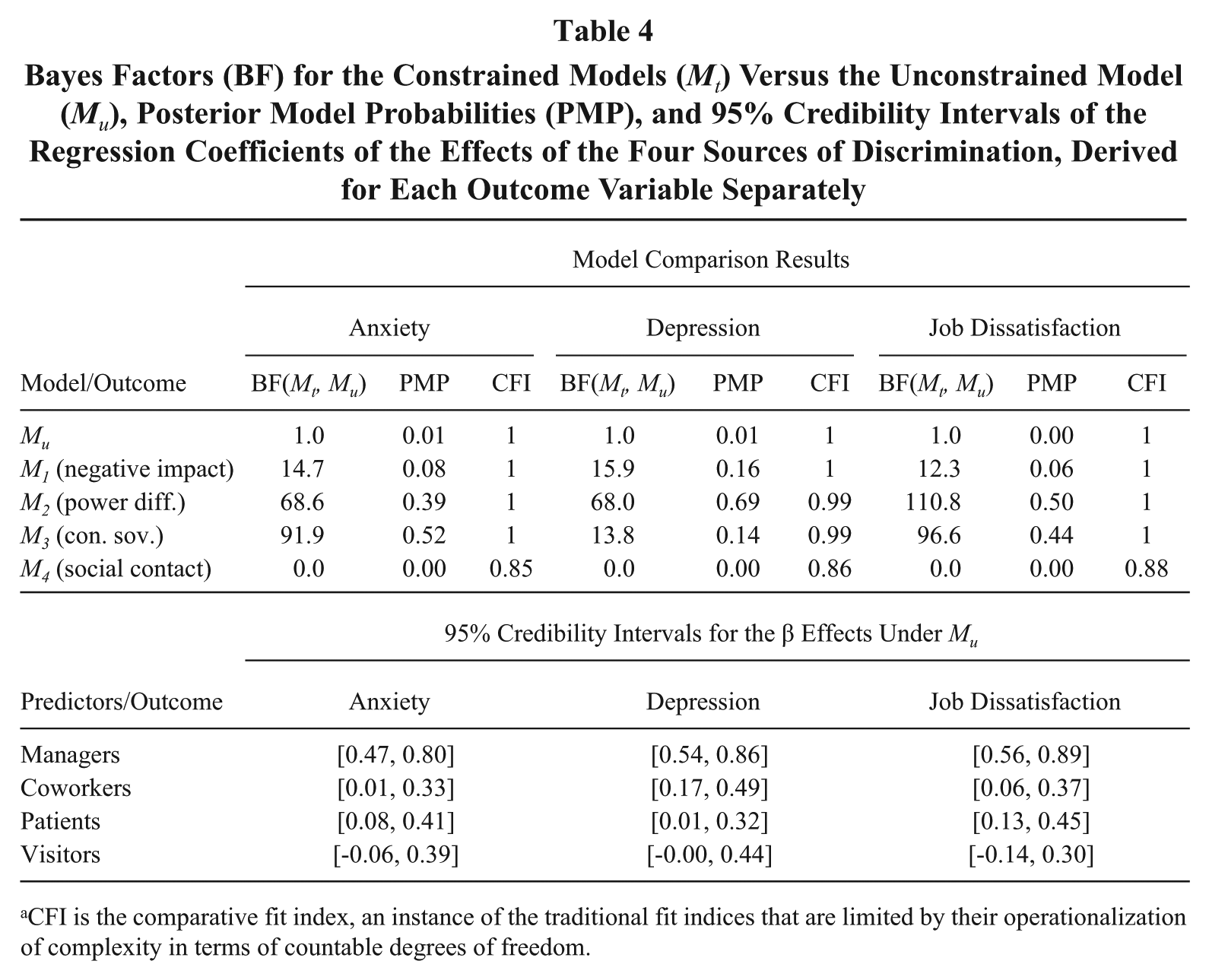
CFI is the comparative fit index, an instance of the traditional fit indices that are limited by their operationalization of complexity in terms of countable degrees of freedom.

To illustrate problems that one might encounter when adopting a traditional model comparison approach to competing order-constrained models, we first look at the resulting CFI values for the different models. Based upon a CFI below the common acceptable fit threshold of 0.95, we can conclude that Model 4 does not show adequate fit to the data, but we also are unable to distinguish between the other models and this for all three outcome variables. They all appear to fit equally well (CFI’s all equal to 0.99 or 1). This result provides us with little conclusive information to determine which of our hypotheses is most supported by the data. In contrast, Bayes factors do provide an informative way of selecting between competing order-constrained models by adequately balancing fit and parsimony.

Table 4 shows that for each outcome there is positive supporting evidence for Model 1 (as indicated by Bayes factor between 12.3 and 15.9), which is consistent with all discrimination sources having a negative impact on well-being. However, the Bayes factors of zero for Model 4 indicate that this model describes the data badly and its constraints do not hold, a result that is in agreement with the CFI-based conclusion and with the 95% credibility intervals of the regression coefficients in the lower panel of Table 4. The Bayesian analysis clearly shows that this social contact hypothesis (i.e., Model 4) underplays the most impactful source of discrimination in this sample, this being the managers. These results point in the direction of Models 2 and 3.

Based upon the Bayes factors we can conclude that Model 2 receives consistently strong support across the three outcomes, whereas Model 3 receives less support for depression (i.e., Bayes factor of 13.8 compared to Bayes factors of over 90 for anxiety and job satisfaction). When inspecting the posterior model probabilities, we observe that for depression Model 2 (the power differential hypothesis) is best supported (i.e., proportional weight of .69 in the set of models). But for both anxiety and job dissatisfaction Model 2 and Model 3 receive roughly equally strong support with posterior model probability of 0.39 versus 0.52 and 0.50 versus 0.44, respectively; this corresponds to about equal odds for both models as represented by Bayes factors between Model 2 and 3 of 0.75 and 1.13. What these two models share is that they put managers first and visitors last in the impact ordering of discrimination sources. There is not enough evidence to decide between the relative strength of the effect of discrimination from patients and that from coworkers on anxiety or job satisfaction. Whereas a significance testing approach would force us to make a binary decision, the Bayes factor approach does not force us to choose between these two models; instead we can quantify how much weight or belief we attach to each model in the form of these posterior model probabilities. Bayesian methods give a clearer view of uncertainty in terms of probability and we should not shy away from such statements.

Based upon these sample data, we can conclude that there is no strong support for the social contact hypothesis and that we are to gauge between two hypotheses, the power differential and consumer sovereignty and patient’s rights propositions. Further theoretical developments might want to concentrate on their mutual overlap, but also try to explore whether other measures of well-being yield a more clear differentiation between the two hypotheses (as is the case for depression).

Application 2: Interpretations of the Karasek Theory of Psychological Strain

Karasek’s (1979) job strain model is highly influential in the occupational psychology and the wider management and work literature. It posits that psychological strain or stress is related to both the demands placed on an individual and their degree of job control or discretion. The core argument is typically based on energy depletion: demands place the individual in a motivated or energized state, while the degree of control modulates the transformation of potential energy into action. Accordingly, job demands are positively related to strain as they trigger it, and job control negatively as this enables the individual to more readily respond to the demands. As energy becomes depleted, strain intensifies.

Here we compare different hypotheses about how the relative order of magnitude of the effects of job control and demands depends on the specific well-being outcome dimension (e.g., the effect of demands overrules the effect of control for anxiety, but it’s the other way around for their effects on job satisfaction). These are multivariate order hypotheses because effects are compared not only between predictors but also across outcomes, and the expected orderings between predictors are not consistent across the different outcomes. Order constraints will be formulated between six regression coefficients, β X . Y , based on two different predictor X-variables—control (Con) and demands (Dem)—and three different outcome Y-variables—anxiety (Anx), depression (Dep), and job dissatisfaction (Jds). For example, β C o n . A n x denotes the effect of control on anxiety.

Model 1: Directional effects model (M₁)

The first interpretation of Karasek’s theory that we investigate is limited to a priori expectations about the direction of the effects of control and demands. Because more control is expected to result in a positive effect on a worker’s well-being and more demands is expected to result in a negative effect on a worker’s well-being, the regression coefficients are expected to have the following signs:

β C o n . A n x < 0 , β D e m . A n x > 0 ,

β C o n . D e p < 0 , β D e m . D e p > 0 ,

β C o n . J d s < 0 , β D e m . J d s > 0 .

Table 5 provides the order constraints of this model, and its two competitor models below, as implemented in BIEMS.

OPEN IN VIEWER

Table 5

Order-Constrained Models as Implemented in BIEMS for Application 2

Model	Order Constraints in BIEMS
M1: Directional effects model
	α ( 1 , 1 ) < 0 , α ( 1 , 2 ) < 0 , α ( 1 , 3 ) < 0 ,
	α ( 2 , 1 ) > 0 , α ( 2 , 2 ) > 0 , α ( 2 , 3 ) > 0
M2: Warr’s circumplex model
	− α ( 1 , 1 ) < α ( 2 , 1 ) , − α ( 1 , 2 ) > α ( 2 , 2 ) , − α ( 1 , 3 ) > α ( 2 , 3 ) ,
	− α ( 1 , 1 ) < − α ( 1 , 2 ) , − α ( 1 , 1 ) < − α ( 1 , 3 ) ,
	α ( 2 , 1 ) > α ( 2 , 2 ) , α ( 2 , 1 ) > α ( 2 , 3 )
M3: Self-determination model
	− α ( 1 , 1 ) > α ( 2 , 1 ) , − α ( 1 , 2 ) > α ( 2 , 2 ) , − α ( 1 , 3 ) > α ( 2 , 3 ) ,
	− α ( 1 , 1 ) > − α ( 1 , 3 ) , − α ( 1 , 2 ) > − α ( 1 , 3 )

a

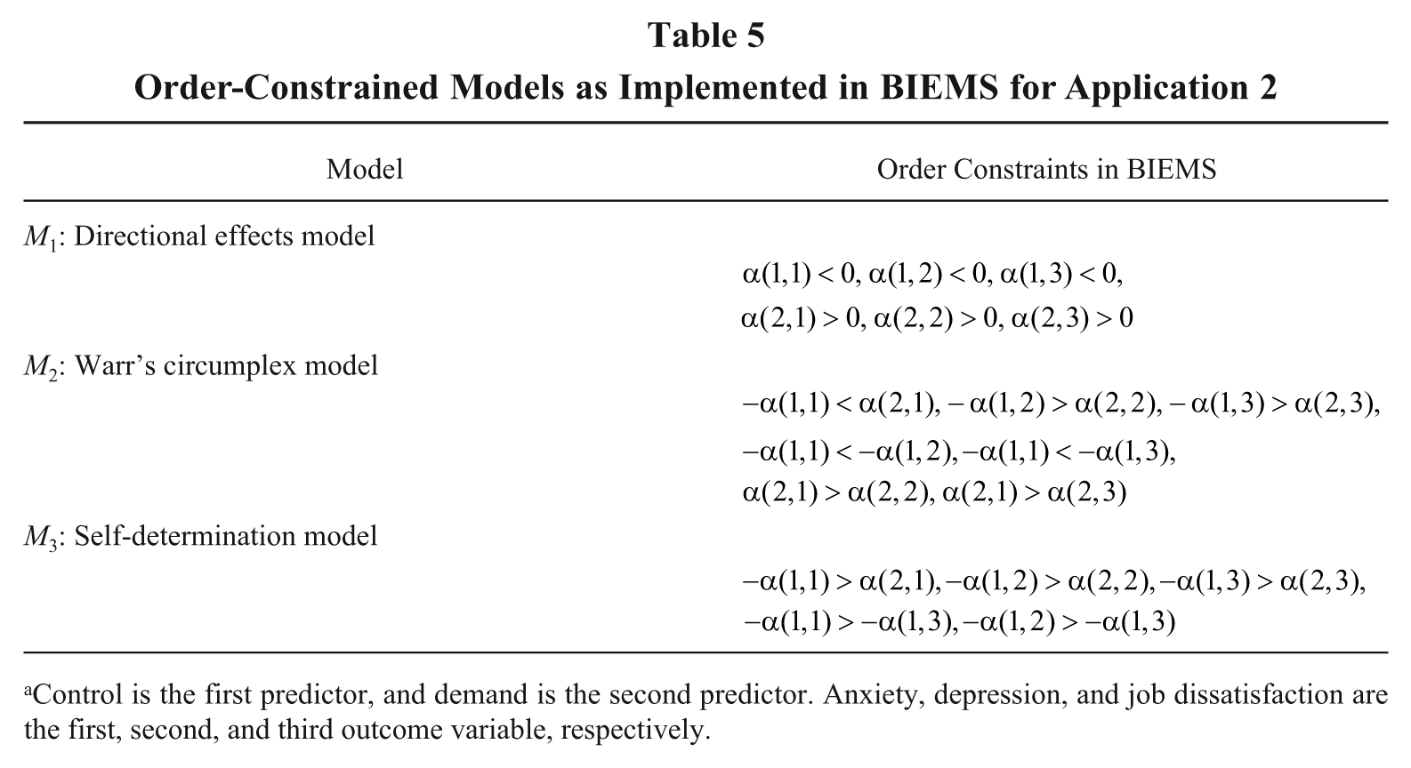
Control is the first predictor, and demand is the second predictor. Anxiety, depression, and job dissatisfaction are the first, second, and third outcome variable, respectively.

Model 2: Warr’s circumplex model (M₂)

The second interpretation contains the same constraints as Model 1, but adds a theoretical layer that builds on expectations that the ordering of the effects of demands and control will not be the same across the different dimensions of well-being. Following the circumplex theory of affect (Russell, 1980), we may differentiate feelings of anxiety from depression. Anxiety combines low pleasure with high arousal, while its opposite contentment is associated with higher levels of pleasure and low arousal. In contrast, depression involves feelings of low pleasure and low mental arousal, and enthusiasm entails feelings of high pleasure and high mental arousal. According to Warr (2007), job demands are more likely to generate anxiety than depression, whereas the frustration and loss of autonomy associated with jobs with low control is more likely to lead to depression. Job satisfaction is concerned only with the pleasure dimension and not arousal. Therefore, it can be anticipated to behave more like depression than anxiety, as the pleasure of work is depleted more by high demands than is the contentment. Thus, within each outcome variable, we expect the following relative magnitude ordering of effects:

− β C o n . A n x < β D e m . A n x ,

− β C o n . D e p > β D e m . D e p ,

− β C o n . J d s > β D e m . J d s .

A minus is included in front of, β C o n . A n x , β C o n . D e p and β C o n . J d s because these effects are expected to be negative. Across the three outcome variables we expect that the effects of control are strongest for job dissatisfaction compared to the other two outcomes, whereas the effects of demands are expected to be strongest for anxiety. This yields:

( − β C o n . A n x , − β C o n . D e p ) < − β C o n . J d s ,

β D e m . A n x > ( β D e m . D e p , β D e m . J d s ) .

These last order constraints must be specified separately in BIEMS for each term within the brackets [e.g., β D e m . A n x > ( β D e m . D e p , β D e m . J d s ) should be implemented as β D e m . A n x > β D e m . D e p and β D e m . A n x > β D e m . J d s ] (see Table 6).

OPEN IN VIEWER

Table 6

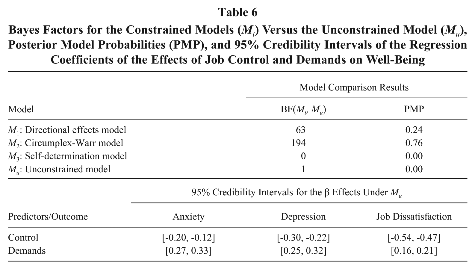
Bayes Factors for the Constrained Models (M_t) Versus the Unconstrained Model (M_u), Posterior Model Probabilities (PMP), and 95% Credibility Intervals of the Regression Coefficients of the Effects of Job Control and Demands on Well-Being

		Model Comparison Results
Model		BF(Mt, Mu)	PMP
M1: Directional effects model		63	0.24
M2: Circumplex-Warr model		194	0.76
M3: Self-determination model		0	0.00
Mu: Unconstrained model		1	0.00
Predictors/Outcome	95% Credibility Intervals for the β Effects Under Mu
	Anxiety	Depression	Job Dissatisfaction
Control	[-0.20, -0.12]	[-0.30, -0.22]	[-0.54, -0.47]
Demands	[0.27, 0.33]	[0.25, 0.32]	[0.16, 0.21]

Model 3: Self-determination model (M₃)

The third model contains the same constraints as Model 1 but adds different order constraints than Model 2. This interpretation is inspired by self-determination theory, according to which autonomy, along with competence and connectivity, are basic needs of workers (Deci & Ryan, 1995). Although demands may indirectly fulfill basic needs such as honing competence, control directly fulfills the basic need for autonomy, and as such we might hypothesize that control will have a greater effect on well-being than will demands:

− β C o n . A n x > β D e m . A n x ,

− β C o n . D e p > β D e m . D e p ,

− β C o n . J d s > β D e m . J d s .

Although no specific ordering is expected regarding the relative effects of demands’ across the three outcome variables, control is expected to have a stronger effect on anxiety and depression than on job dissatisfaction:

( − β C o n . A n x , − β C o n . D e p ) > − β C o n . J d s .