Restricted Variance Interaction Effects: What They Are and Why They Are Your Friends

Abstract

Although interaction hypotheses are increasingly common in our field, many recent articles point out that authors often have difficulty justifying them. The purpose of this article is to describe a particular type of interaction: the restricted variance (RV) interaction. The essence of the RV interaction is that, as the value of one variable in a system changes, certain values of another variable in the system become less plausible, thus restricting its variance. This, in turn, influences relationships between that variable and other variables. These types of interactions are quite common, even if they are not recognized as RV interactions, and they exist at every level of analysis. The advantage of the RV interaction is that, as compared with other interaction types, it is relatively simple to justify. The different forms of RV interaction do, however, contain complexities of which a researcher must be aware. This article explains and illustrates the forms that RV interactions can take and their often counterintuitive implications. It also describes how one should go about testing them. Our intention is to help researchers strengthen and focus their interaction arguments.

Keywords

multilevel modeling/hierarchical research methods statistical methods personality

Interaction models are increasingly common in the organizational sciences. Indeed, it would appear that this trend has been in place for some time (cf. Aguinis, 1995; Cortina, 1993, 2003). Even a cursory review of any of our top journals will show that it is rare to come across an empirical article (or a theoretical one) that does not include an interaction hypothesis of some sort (Aguinis, Edwards, & Bradley, 2017).

With this popularity has come concern over what appears to be confusion regarding the conceptualization and testing of interaction models. For example, Andersson, Cuervo-Cazurra, and Nielsen (2014) point out that authors sometimes justify interactions by arguing for the effect of the moderator on the dependent variable (DV) even though such an argument is not only insufficient but unnecessary for many types of interactions. Holland, Shore, and Cortina (2017) point out that authors sometimes justify what amounts to a particular sign for the product term weight in a moderated regression equation, without considering the fact that the pattern of an interaction is determined not only by the product term weight but also by the weights attached to the variables that make up the product. As another example, in cross-level research, authors sometimes argue that because a putative moderator variable is likely to vary across units, within-unit relationships will vary across levels of the moderator (e.g., Chowdhury & Endres, 2010). Lack of clarity regarding the nature of interaction effects may lead us to pursue interaction effects that do not really have any basis, which would explain why effect sizes for interactions are often relatively small (Aguinis, Beaty, Boik, & Pierce, 2005; Murphy & Russell, 2017).

In a recent editorial, Cortina, Köhler, and Nielsen (2015) argued that a particular category of interaction hypothesis—the restricted variance (RV) interaction—is quite common in international business research, but most international business researchers do not recognize it. The essence of the RV interaction is that, as the value of one variable in a system changes, certain values of another variable in the system become less plausible, thus restricting its variance. This, in turn, influences relationships between that variable and other variables. Thus, a variable Z acts as a moderator of the relationship between X and Y because the variance of X or Y is compressed at certain levels of Z and this compression affects the X-Y relationship. As we argue here, just as these sorts of interactions are common in international business phenomena, so are they common in the organizational sciences more generally. Moreover, they are not specific to any particular level of analysis. Cortina et al. gave examples at the country and organizational levels, but RV interactions can also be found at the between-unit level, the between-person level, and even the within-person level.

One of the great advantages of RV interactions is that they are relatively simple to conceptualize and defend. One need only explain why it is that values for one variable are implausible at certain levels of a moderator and why, at other levels of the moderator, values of the first variable are free to vary and to covary with other variables. The classic example—and one with which many are familiar—is the Situation Strength × Personality interaction proposed by Mischel (1973) and reviewed by Meyer, Dalal, and Hermida (2010), in which the personality-behavior relationship is weak in strong situations because of the lack of variance in behavior in such situations. In weak situations, behavior is free to vary, and this variance is explained by personality.

This logic can be extended to many phenomena in the organizational sciences. For example, Ilies, Scott, and Judge (2006) hypothesized that intraindividual increases in positive affect would be associated with increases in organizational citizenship behaviors (OCBs) but that this relationship would be weaker for those high in trait agreeableness. These authors argued that positive affect is necessary for those low in agreeableness to engage in OCBs. Those high in agreeableness engage in OCBs regardless of affect. Although Ilies et al. did not make RV arguments, their interactions could be framed in such terms. Y has less variance (i.e., it is uniformly high) when the moderator is high, in which case Y has less of a relationship with X. When the moderator is low, Y has more variance, and that variance is explained by X.

As we show, there are a great many other examples in management, and they exist at every level of analysis. Because an RV phenomenon is relatively easy to describe and justify, it is our contention that a broader appreciation of RV interactions would result in stronger justifications and tests of interaction hypotheses.

The purpose of the present article is to explain and illustrate the nature and testing of RV interactions in organizational research. After a brief description of interactions more generally, we show the different forms that RV interactions can take and the sorts of arguments that should accompany them. We also differentiate RV interactions from range restriction phenomena, which are entirely different. We then detail the empirical evidentiary requirements of such interactions for a variety of designs and provide recommendations to guide future researchers in identifying, justifying, testing, and reporting RV interactions.

What Are RV Interactions?

Interaction effects describe a relationship in which the effect of a predictor variable (X) on an outcome variable (Y) depends on the level of the moderating variable (Z) or, more generally, the relationship between two variables is contingent on some condition. At the least, a moderator variable affects the strength¹ of the X-Y relationship and thus helps researchers identify the boundary conditions under which a given relationship exists. Specifically, moderator variables explain when (or for whom) an independent variable (IV)–DV relationship exists or how strong it will be under different conditions (e.g., Andersson et al., 2014; Frazier, Tix, & Barron, 2004).

RV interactions are a specific type of interaction effect that stipulates a particular reason for the effect of the moderator on the X-Y relationship. Specifically, in an RV interaction, the variance of X or Y changes as a function of Z. In other words, the variance of X or Y is restricted (or enhanced) as a function of Z, and this restriction/enhancement of variance affects the magnitude (though probably not the sign) of the X-Y relationship. For example, Mischel (1973) postulated that the strength of a given situation constrains the behavior or cognitions in which an individual engages, potentially overriding the effect of personality differences:

Psychological “situations” and “treatments” are powerful to the degree that they lead all persons to construe the particular events the same way, induce uniform expectancies regarding the most appropriate response pattern, provide adequate incentives for the performance of that response pattern, and instill the skills necessary for its satisfactory construction and execution. . . . Individual differences can determine behavior in a given situation most strongly when the situation is ambiguously structured . . . so that subjects are uncertain about how to categorize it and have no clear expectations about the behaviors most likely to be appropriate (normative, reinforced) in that situation. . . . Conversely, when subjects expect that only one response will be reinforced . . . then individual differences will be minimal and situational effects prepotent. (p. 276)

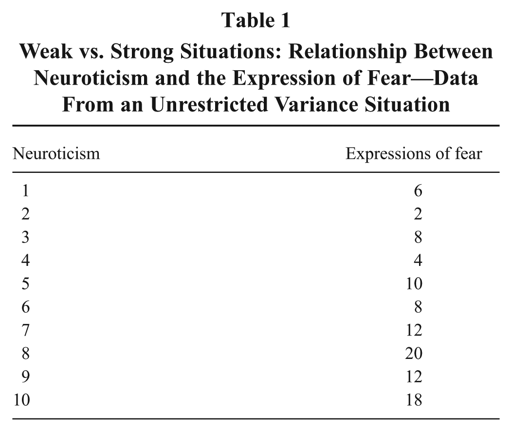
To illustrate, consider the data in Tables 1 and 2. The data in Table 1 reflect a positive relationship between neuroticism and the expression of fear. Let us suppose that these data were collected in a “weak” situation, and let us then ask what we would expect to happen if data for the same variables were collected in a situation in which there were strong norms against expressing fear (e.g., an army platoon briefing, a huddle in the National Football League). Presumably, the variance in a stable individual difference variable would not be influenced by the situation (we discuss the effects of selection in a later section), but the variance in expression of fear would be affected by norms. Specifically, the norms against fear expression would have the same sort of effect as would severity bias: suppressing all values but suppressing large values more than small values. The data in Table 2 reflect this downward compression on the DV. The DV data in Table 2 were created by multiplying the DV values in Table 1 by 0.4. This transformation reduces large values more than it reduces small values, as would be the case for a phenomenon such as that described by Mischel (1973). Nevertheless, the pattern of the X-Y relationship is the same at the two levels of the moderator in the sense that the rank order of Y relative to X remains unchanged, but higher values of the Y variable are unlikely in the high strength condition because they have been compressed downward. As a result, Y has less variance in the strong condition than in the weak condition.

Table 1

Weak vs. Strong Situations: Relationship Between Neuroticism and the Expression of Fear—Data From an Unrestricted Variance Situation

Neuroticism	Expressions of fear
1	6
2	2
3	8
4	4
5	10
6	8
7	12
8	20
9	12
10	18

Table 2

Weak vs. Strong Situations: Relationship Between Neuroticism and the Expression of Fear—Data From a Restricted Variance Situation

Neuroticism	Expressions of fear
1	2.4
2	.8
3	3.2
4	1.6
5	4
6	3.2
7	4.8
8	8
9	4.8
10	7.2

If we conduct these regressions separately, we get the results in Figures 1 and 2. We see that the X-Y slope is 1.58 in the weak condition but 0.63 in the strong condition. Note that the difference in these slopes is directly proportional to the differences in the standard deviations of Y at the two levels of the strength variable. The reduction in the standard deviation of Y by 60% results in a corresponding reduction in the covariance of 60%. Because the regression weight is equal to

Figure 1

Plot of the Regression of Fear Expressions Onto Neuroticism: Weak Situation

Figure 2

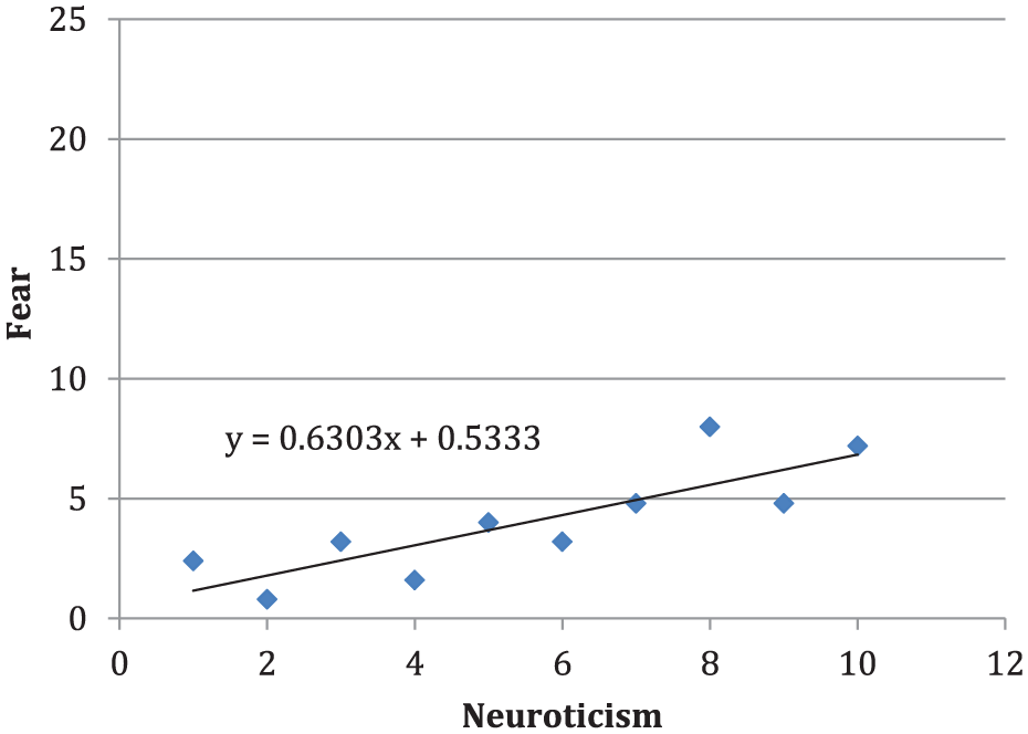
Plot of the Regression of Fear Expressions Onto Neuroticism: Strong Situation

b = \frac{C O V_{x y}}{S_{x}^{2}},

the weight must also be reduced by 60%. Thus, the magnitude of the interaction is tied to the amount of restriction (or enhancement).

Now suppose that these two data sets were combined into a single data file with a dichotomous moderator representing situation strength. A moderated regression (see Table 3) shows that the weight for the XZ product (–0.945) is significantly different from zero. It is in fact negative because the X-Y slope is closer to zero in the strong condition than in the weak. These differences in weights are due to compression of the DV. This is the RV interaction effect.

Table 3

Moderated Regression Results With Weights and R² at Each Step

Predictors	b	SD	t	p
Neuroticism	1.1	0.225	4.89	.00
Situation strength	−6.0	1.29	−4.63	.00
R² = .728
Neuroticism × Situation Strength	−0.945	0.40	−2.36	.031
ΔR² = .07

There are a number of reasons how and why a moderator might restrict or enhance variance in one or more variables in a system. In the following section, we provide a variety of examples for the reasons that an RV moderator may affect the IV-DV relationship. The commonalities among these examples should illustrate the basis for the theoretical rationale that underlies an RV interaction.

Theoretical Rationales for RV Interactions

To explain how to make a case for an RV interaction, we begin by considering briefly how arguments are made for interaction effects more generally. In arguing for interaction hypotheses, one must make a case that a certain relationship is, in some way, variable or—as Cohen and colleagues (Cohen, Cohen, West, & Aiken, 2003), Arnold (1982), Stone and Hollenbeck (1984), and others put it—conditional. Perhaps the simplest case is that in which Z is a categorical moderator of the X-Y relationship. If Z is truly categorical, then one can argue that the X-Y relationship is different for the different categories because of a stable difference among the categories.

If Z is continuous, then the case is more difficult to make because one cannot draw on qualitative differences among groups (Andersson et al., 2014). In principle, one must argue that the X-Y relationship changes as a function of the moderator. In a bilinear interaction, it must be argued that the X-Y relationship differs by a fixed amount for a given difference in Z. In a quadratic relationship, it must be argued that the X-Y relationship differs by a fixed amount for a given difference in X. For higher-order interactions, it must be argued that lower-order interactions differ by fixed amounts for a given difference in moderators and so on.

Because interaction hypotheses are often coupled with main effect hypotheses, together they form a set that reflects a specific pattern. Defending specific patterns can be quite challenging. Cohen et al. (2003) provided labels and explanations for different combinations of main and interaction effects. Of particular interest for present purposes are the interactions described by Cohen et al. as buffering and interference interactions.

Buffering RV interactions

RV interactions typically involve the weakening of an effect as the moderator changes in a particular direction, with values of Y converging on a certain value as the moderator moves in the “strong” direction. As we discuss later, this is not necessarily the case, but it is the most common form of RV interaction. One pattern that would result from an RV phenomenon would be that associated with a buffering interaction. In a buffering interaction, the moderator Z moderates the X-Y relationship because high levels of Z act as a buffer against the effects of X, reducing the importance of X for Y. The X and Z effects are of opposite sign, but the relationship between either and Y is weaker at higher levels of the other.

Cohen et al. (2003) explain that buffering interactions are common in research involving risk factors and protective factors. A certain physical characteristic (e.g., family history of a particular condition) or situational characteristic (e.g., low SES) is associated with undesirable outcomes (e.g., cancer, incarceration), but protective factors (e.g., diet, family support) act as a buffer. In an RV phenomenon, one would argue that the relationship between the risk factor and the outcome is reduced because certain values of the outcome (high values in this case) are unlikely at higher levels of the protective factor. A buffering interaction is characterized by predictors that have weights of opposite sign, and increases in one predictor reduce the slope of the line representing the relationship between the other predictor and the outcome.

Mischel’s (1973) situational strength arguments are buffering arguments (see Figures 1 and 2). Personality drives behavior, but situational characteristics mitigate this influence such that situation strength makes certain behaviors unlikely. Consider our earlier example of neuroticism and fear expression. In informal social situations, these two variables are positively related. In settings that impose a norm of (apparent) fearlessness, expression of fear is rare, and neither neuroticism nor anything else is likely to relate strongly to it. In terms of weights, we would expect a positive weight for neuroticism but a negative weight for strength. The product term would also have a negative weight because the slope representing the relationship between neuroticism and fear decreases as situational strength increases. Situational strength acts as a buffer against the effects of neuroticism on fear expression.

Another sort of buffering RV interaction comes from King and Ahmad (2010), who conducted a field experiment of the effects of Muslim identity on discrimination directed at job applicants. They found that this relationship was positive (i.e., applicants wearing Muslim attire encountered more discrimination) but that it was weaker if the applicant exhibited warmth (which was stereotype disconfirming). Thus, warmth acted as a buffer against the effect of identity on discrimination, with the result being a pattern such as that in Figure 3, which is intended as a plot of the bar chart in Figure 2 of King and Ahmad.

Figure 3

Replotting of the Bar Chart in Figure 2 of King and Ahmad (2010) in Which Warmth Acted as a Buffer Against the Effect of Identity on Discrimination

Our Figure 3 shows that the amount of discrimination experienced by Muslim applicants depends on whether the applicant exhibits warmth. However, we can see from King and Ahmad (2010) that discrimination was uniformly low for applicants who exhibited warmth. Warmth created a strong situation that kept discrimination low regardless of applicant attire. Only in the weak situation (no warmth information) was discrimination free to vary, in this case as a function of identity/attire.

As another example, Marcel, Cowen, and Ballinger (2017) examined the relationship between board use of an interim CEO and audience attitudes regarding board performance. They hypothesized that this relationship would be negative but that it would be moderated by the suddenness of the departure of the previous CEO such that audiences (credit agencies, securities analysts, etc.) would react less negatively to the use of an interim CEO if the departure was sudden. This could be recast in RV terms. When the departure of the previous CEO is sudden, audiences are more sympathetic to the short-term bind in which boards find themselves, so their attitudes toward board actions are (relatively) uniformly positive. When departure was not sudden, then attitudes have more variance, which can be explained by reliance (or not) on an interim CEO.

Interference RV interactions

A second category of interaction effect described by Cohen et al. (2003) is the interference interaction. In an interference interaction, the predictor and moderator have effects in the same direction, but the interaction works in the opposite direction. If the main effects are positive, then values of the outcome are restricted to high levels when either predictor is high. If the main effects are negative, then the opposite is true. In either case, the interference pattern is produced because values of the outcome variable converge upon a certain value at particular levels of one or the other predictor.

The Ilies et al. (2006) example given earlier is an example of an interference interaction. Agreeableness “interferes” with positive affect such that positive affect is not necessary for OCBs among highly agreeable people for whom OCBs are high regardless of affect. As another example, Lyness and Heilman (2006) found that the positive relationship between performance ratings and probability of promotion were stronger for women than for men. Given that the authors also found that men received more promotions than women, this would be an example of an interference interaction in that the main effect of performance ratings is positive, men (coded as 1) were more likely to be promoted than women (coded as zero), and the performance rating-promotion slope was less positive for men, resulting in a negative weight for the product. The interaction is driven by the fact that variance in promotions is restricted when performance ratings are high (i.e., promotion is uniformly high) but much less restricted when performance ratings were low, because men with low ratings were often promoted whereas women with low ratings were not.

At a higher level of analysis, Lu, Liu, Wright, and Filatotchev (2014) hypothesized that in countries with strong market-supporting institutions, prior international experience is less important in determining foreign direct investment (FDI) than it is in countries with weak market-supporting institutions. Strong market-supporting institutions help firms to identify and contact potential customers, navigate regulations, and so on, making prior experience less important. Thus, FDI is uniformly high (i.e., low values are implausible) regardless of a firm’s prior international experience and is therefore only weakly related to it. In countries with weak market-supporting institutions, firms are left to fend for themselves. In such cases, FDI is low for firms with low levels of experience but high for firms with high levels of international experience. Thus, market-supporting institutions interfere with the effects of experience. The interaction between market-supporting institutions and experience can be justified simply by explaining why FDI is uniformly high where strong market-supporting institutions are present and why FDI varies as a function of experience where such institutions are absent.

A very similar argument could be made in support of Hypothesis 3a from Zheng, Singh, and Chung (2017). Where there is high capital market development, firms that wish to exit do so through sell-offs regardless of their political ties. In the absence of capital market development, firms may exit through sell-off or simple dissolution (i.e., there is variance in the manner of exit). Whether they sell off or are merely dissolved depends on political ties.

In all of these examples, as a result of the interfering phenomenon, Y has less variance (i.e., it is uniformly high) when the moderator is high. When the moderator is low, Y has more variance, which is explained by another variable. These examples also show that RV interactions can exist at any level of analysis.

Figure 4 contains data and results consistent with an interference RV interaction. Let us suppose that we hypothesize a model like that of Ilies et al. (2006). When agreeableness is low, OCBs are low or high depending on positive affect. High agreeableness, however, acts as a strong situation, compressing OCB values upward (i.e., low OCB values are implausible regardless of affect). The result is an Affect × Agreeableness interaction such that the weights for the predictors are both positive but the affect-OCB relationship is weaker for those high in agreeableness.

Figure 4

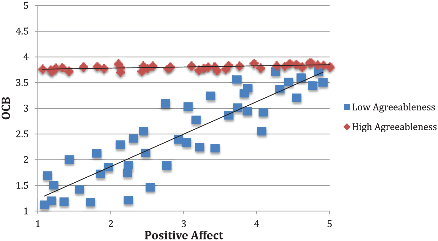
Data and Results Consistent With an Interference Restricted Variance Interaction From Ilies, Scott, and Judge (2006)

In all these cases, the argument for interaction can be simplified or at least augmented by explaining why the DV varies little when the moderator is at a certain level. Fear expression is unlikely in platoon meetings regardless of the personality of the subject. Discrimination is low for applicants who exhibit warmth, regardless of attire. Promotions are high for high performers regardless of gender. OCBs are high for those high in agreeableness regardless of affect. FDI is high in countries with strong market-supporting institutions regardless of firm experience. It is only when the “situation” is weakened (e.g., lack of norm for fearlessness, lack of warmth, low performance, low agreeableness, weak market-supporting institutions) that substantial variance in the DV exists. This variance can then be explained by, for example, neuroticism, identity, gender, affect, and experience.

IV compression RV interaction

In all the examples that we offer, the RV interaction came about as a result of certain values of the DV being implausible at certain levels of the moderator. An RV interaction can, however, also result from compression on the IV. As we explain in a later section, this is entirely different from the restriction-of-range problem that is common in selection research (see also Aguinis et al., 2017). In any case, the result of IV compression is different from that of compression on the DV, and as we explain, these results are not widely appreciated.

Consider once again the examples in Tables 1 and 2. Let us suppose that, for some reason, instead of wishing to predict fearful expressions from neuroticism, situation strength, and their product, we wished to predict neuroticism from fearful expressions, situation strength, and their product. Suppose further that the same situational factor was at work such that the values of the fear expression variable (now the predictor) were compressed downward. If we then performed these regressions separately for each of the two levels of situation strength, we would have the plots in Figures 5 and 6. As can be seen from these plots, the values of Y are uniformly low when X is low, just as in the case with Figures 1 and 2. However, unlike Figures 1 and 2, Figures 5 and 6 show that variability in Y does not increase as a constant function of X. Instead, variability increases until the (compressed) limits of X are reached, and then variability in Y drops back down.

Figure 5

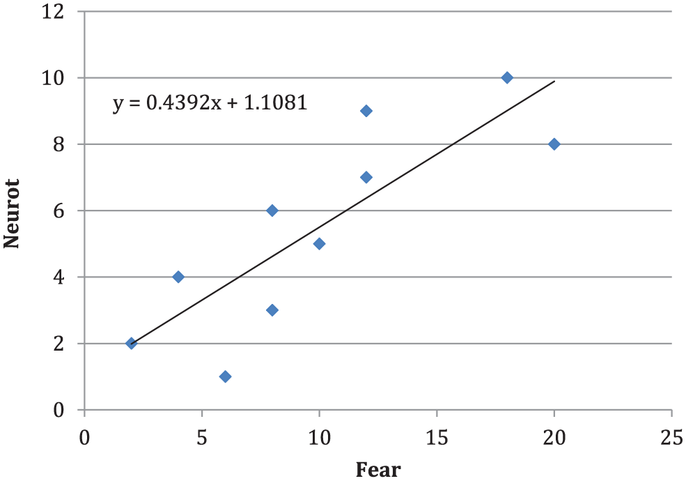
Plot of the Regression of Neuroticism Onto Fear Expressions: Weak Situation

Figure 6

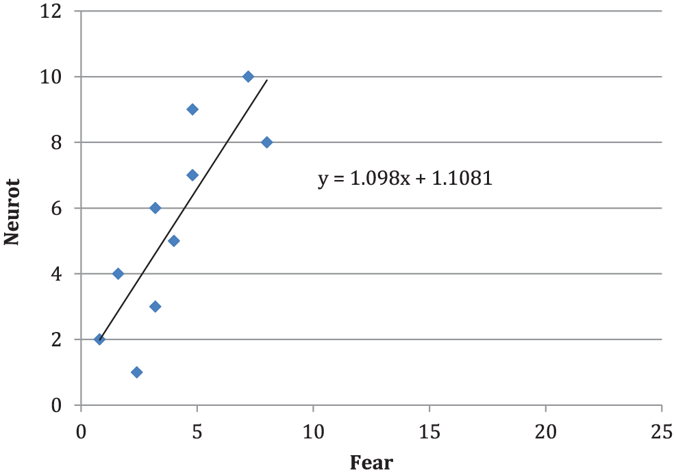
Plot of the Regression of Neuroticism Onto Fear Expressions: Strong Situation

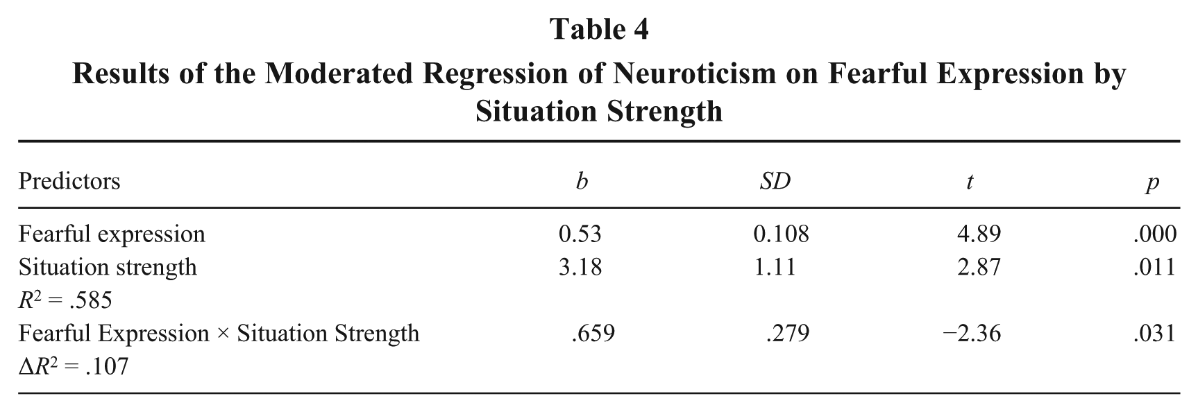
The results of the moderated regression, based on centered variables, are presented in Table 4 and plotted in Figure 7. If we compare these results with those in Table 3, we see that the weight for the product is now positive and the ΔR² is different. However, the results of the t tests for the interaction are identical in the two examples. Thus, although compressing the values of the IV instead of the DV changed the magnitude of the interaction, the change in the standard error of the product was proportional, resulting in the same t and p values. If this were one’s only interest, then it makes no difference whether the compression is in the IV or the DV.

Table 4

Results of the Moderated Regression of Neuroticism on Fearful Expression by Situation Strength

Predictors	b	SD	t	p
Fearful expression	0.53	0.108	4.89	.000
Situation strength	3.18	1.11	2.87	.011
R² = .585
Fearful Expression × Situation Strength	.659	.279	−2.36	.031
ΔR² = .107

Figure 7

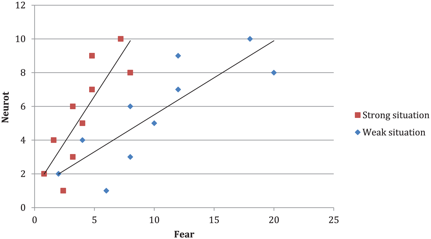
Plot of the Regression of Neuroticism Onto Fear Expressions

However, the weight for the product indicates that the slope representing the relationship between expressions of fear and neuroticism is steeper (i.e., more positive) in the strong situation. Recall from the regression of fearful expressions onto neuroticism that the difference in weights was proportional to the difference in covariances produced by the compression. In the regression of neuroticism onto fearful expressions, the covariances are affected in exactly the same way as they were in the earlier example. They must be because

C O V_{x y} = \frac{\sum (X - \bar{X}) (Y - \bar{Y})}{N - 1} = \frac{\sum (Y - \bar{Y}) (X - \bar{X})}{N - 1} = C O V_{y x} .

But because the compression in the present example occurs on the IV, the denominator of b is also affected. Per Equation 1, the unstandardized regression weight is covariance divided by variance of X, and whereas the covariance in the strong situation is 0.4 of its value in the weak situation, the variance of X in the strong situation is 0.4² of its value in the weak situation. Thus, the denominator of b is reduced by a greater amount than the numerator is, and b is therefore smaller in the weak situation by a factor of .4² / .4 = .4.

We stated earlier that most RV interactions are either buffering interactions (main effects of opposite sign) or interference interactions (interaction effect of different sign from both main effects) because most RV interactions involve restriction on the DV (as opposed to enhancement). If restriction occurs on the IV, however, the interaction may be of the synergistic sort, as in this example. All three terms in the regression have the same sign, meaning that the slope for one predictor gets more extreme as the other predictor increases.

We mentioned earlier that the effects of IV compression are poorly understood. Note that the synergistic pattern described in the previous paragraph is the opposite pattern from that proposed by most authors of models in which IV restriction is implied. Consider the left-hand side of the model by Ozer (2011). OCBs directed at individuals and organizations (i.e., OCBIs and OCBOs) are positively related to team member exchange (TMX) but only if there is sufficient task autonomy: “Employees will be able to engage in OCBIs [and OCBOs] to their coworkers and thus enjoy stronger TMX relationships with them only when they have sufficient freedom to perform such behaviors” (p. 1329). Thus, the authors expect a positive main effect for OCB and a negative moderating effect of situation strength (i.e., lack of autonomy) owing to RV in OCB when strength is high. This would be either a buffering or interference interaction depending on the main effect of situation strength, but it would not be a synergistic interaction.

If, in fact, OCBs are positively related to TMX but are uniformly low when situation strength is high, then we would actually expect the OCB-TMX slope to be steeper when situation strength is high, rather than shallower, as the authors seem to propose. This type of confusion about RV interactions is nearly universal, as it is generally assumed in the literature that the effects of RV would be the same regardless of where in the model the restriction occurs. As we show, however, this is not the case.

As another example, consider the literature on the ideal employee factor. Schmit and Ryan (1993) showed that personality measures administered to nonapplicants exhibited the expected five-factor structure, but measures administered to job applicants exhibited a sixth factor related to the desire to appear as the “ideal employee.” These authors suggested that employees who are motivated to do so (i.e., applicants) tend to inflate their responses, particularly to items whose relevance to the workplace is obvious. If this were true, then we would expect upward compression of personality scores for applicants. If personality were used as a predictor of grade point average (e.g., Schmit, Ryan, Stierwalt, & Powell, 1995), we would expect a synergistic interaction such that the positive relationship between, say, conscientiousness and grade point average is stronger in the strong (i.e., applicant) condition because of the effects of compression on the covariance relative to its effects on the variance of conscientiousness.

Of course, this means that enhancement on the IV also has counterintuitive effects. Let us once again consider the regression of neuroticism onto expressions of fear, but let us begin with the data in Table 2. Suppose that a third variable enhances the variance of fear expression and all values are increased by a factor of 2.5. Thus, large values are increased by a greater amount than small values are, and we have the data in Table 1. This results in an increase in covariance from 5.78 to 14.44 (a factor of 2.5). s²_x, however, increases by a factor of 2.5² = 6.25, from 5.26 to 32.89. Thus, this enhancement on X increases the denominator in Equation 1 by a greater amount than the numerator (2.5² rather than 2.5), and the b value is therefore reduced by a factor of 1 / 2.5 = 0.4: in this case, from 1.098 to .439.

Restriction on both the IV and the DV

It should be clear from our previous discussion that restriction on the IV and the DV by the same factor will not produce an interaction. In such a case, the covariance and the variance of X change by exactly the same amount, and b is unaffected. This can be seen by first considering the effect of compression on the numerator of Equation 2. Compression would reduce deviation scores for X and Y, with corresponding reductions in deviation score cross products. If one then considers the effect of compression on the denominator of Equation 1, one sees that squared deviation scores for X would be reduced by the same amount. Thus, the numerator and denominator of Equation 1 would be reduced by the same amount, and b would remain the same.

Consider the first stage of the mediation model presented by Ozer (2011). We quoted page 1329 of that article to make a point about compression of the IV, but the entire quote from Ozer is as follows: “Employees will be able to engage in OCBIs [and OCBOs] to their coworkers and thus enjoy stronger TMX relationships with them only when they have sufficient freedom to perform such behaviors and engage in social exchange with their coworkers [italics added]” (p. 1329). Thus, the author suggests that situation strength compresses values of OCB and TMX. If the compression effect is similar for these two variables, then in fact situation strength should not moderate their relationship.

If the restricting phenomenon affects the IV and DV by different amounts, b will differ by an amount proportional to the difference in factors by which the IV and DV variabilities are reduced. Our theories are generally not strong enough to suggest point (as opposed to directional) hypotheses, so it is unlikely that an author could base hypotheses on specific differences in compression. We simply wish to make clear that if compression of a certain amount is expected on the IV and the DV, then no interaction should result.

Three-way RV interactions

RV phenomena also produce triple-product interactions. Consider once again Figure 4, which contains an interference interaction intended to mimic the hypotheses of Ilies et al. (2006). OCB is uniformly high for those high in agreeableness but varies with positive affect for those low in agreeableness. But what if there were a unit- or organization-level variable that trumped inter- or intraindividual-level phenomena? Suppose that the norms for citizenship behavior were very strong in one unit of an organization. In such a unit, OCB might be uniformly high regardless of positive affect and agreeableness, and we would see a plot like that in Figure 8.

Figure 8

Triple-Product Restricted Variance Interactions: Organizational Norms for Citizenship Behavior as a Strong Situation

Taken together, these plots suggest that variance in OCB is low if either norms or agreeableness is high. Norms could be said to interfere with the Affect × Agreeableness interaction by compressing OCB values regardless of either. Only if norms and agreeableness are both low is OCB free to covary with intraindividual factors such as affect. We might label this a second-order interference RV interaction (for another example, see Hypothesis 4a of Zheng et al., 2017).

Nonlinear and other RV forms

RV phenomena can also produce nonlinear effects. A ceiling effect is an RV phenomenon such that large values, usually of the outcome variable, are implausible. The true score of a given entity can be observed only if it is less than or equal to the “ceiling threshold” (Wang, Zhang, McArdle, & Salthouse, 2008). If a predictor is positively related to such a variable, then one will observe artifactual nonlinearity such that the X-Y relationship weakens when values of Y begin to hit its threshold, the reason being that high and very high values are compressed, thus restricting the variance of Y at higher levels of X. The result of such a phenomenon would be a scatterplot such as that in Figure 9.

Figure 9

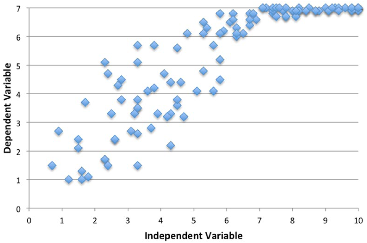
Example of Nonlinear Restricted Variance Interaction

This form of variance restriction results in a positive weight for X but a negative weight for the polynomial term. This is a form of buffering effect in that the ceiling acts as a buffer of the X-Y relationship. Floor effects operate similarly. The true score can be observed only if it is greater than or equal to the threshold value, at which point any negative relationship with this variable would weaken.²

Nonlinear RV phenomena can be more complicated still. The “glass ceiling” effect in the workplace is a form of RV nonlinear interaction. For men, better credentials or experience is associated with more advancement. For women, this may be true up to a point, but then a ceiling effect appears, rendering higher-outcome variable values unlikely. Thus, for men, the relationship is linear and positive, whereas for women, the relationship is positive but concave downward because of RV at high levels of X. Put another way, the ceiling buffers the effect of credentials for women, thus limiting the variance of advancement for qualified women but not for qualified men. RV reasoning such as this could have been used to augment the arguments of Cotter, Hermsen, Ovadia, and Vanneman (2001) for glass ceiling effects for women. This reasoning also would have suggested a particular analysis strategy, beginning with a moderated regression (or random coefficient model in the case of Cotter et al., 2001) that included a Gender × Experience² term.

Conditional indirect effects containing RV interactions

Conditional indirect effect models (also known as moderated mediation models or models integrating moderation and mediation [MiMMs]) have become increasingly popular over the past 20 years. Such models are mediation models in which at least one path is moderated (Preacher, Rucker, & Hayes, 2007). These models, too, can result from RV phenomena. The multivariate nature of such models creates some unique RV issues.

Edwards and Lambert (2007) distinguished among several types of conditional indirect effect models or models integrating moderation and mediation. All of the models discussed by Edwards and Lambert share the same X → M → Y core but vary in the location of the moderation. Holland et al. (2017) found that the most common is the first-stage (X → M) moderation model. Consider as an example a portion of the model presented by Zhang and Bartol (2010). The authors argued that psychological empowerment mediated the effect of empowering leadership on intrinsic motivation. Furthermore, empowerment role identity (the degree to which one views oneself as wanting empowerment) moderates the relationship between empowering leadership and psychological empowerment. The authors reported that although empowering leadership and empowerment are positively related, there are those who have no interest in being empowered. For such people, empowering leadership is less likely to lead to empowerment. This argument could be recast in RV terms. For those with low empowerment role identity, empowerment is low (and therefore has little variance) regardless of leadership. For those high in empowerment role identity, empowerment varies, and this variation can be explained with empowering leadership. As a result of this first-stage RV interaction, the indirect effect of empowering leadership on intrinsic motivation is stronger for those high in empowerment role identity. This argument requires only an explanation for why empowerment is uniformly low for some people, why leadership explains variance in empowerment for others, and why empowerment then leads to motivation.

As discussed earlier, RV effects differ depending on whether the restriction occurs in the IV or the DV. This is particularly important in conditional indirect effect models because the mediator serves as the DV in one equation and the IV in another. If the moderator restricts variance in X (the exogenous variable), then this restriction has implications for all the effects of X. In a partial mediation model with first-stage moderation, RV in X must influence the effect of X on M and the direct effect of X on Y. Thus, a mediation model such as that from Ozer (2011) must be what Edwards and Lambert (2007) call a direct-effect and first-stage moderation model rather than merely a first-stage moderation model.

If instead the moderator restricts variance in M, then this has implications for the first and second stages of the mediation. As we saw earlier, compression on the outcome variable in a relationship weakens its relationship with its predictor, but compression on the predictor variable strengthens its relationship with its outcome. Consider once again the Zhang and Bartol (2010) model. If variance in empowerment is low for those low in role identity, then there should be an Empowering Leadership × Identity interaction as the authors hypothesize (i.e., X-M slope weakens as compression increases). In addition, however, there should be an Identity × Empowerment interaction on motivation such that the empowerment → motivation relationship is stronger for those low in role identity because of compression on what is now the IV. We might therefore expect a situation such as that depicted in Figure 10.

Figure 10

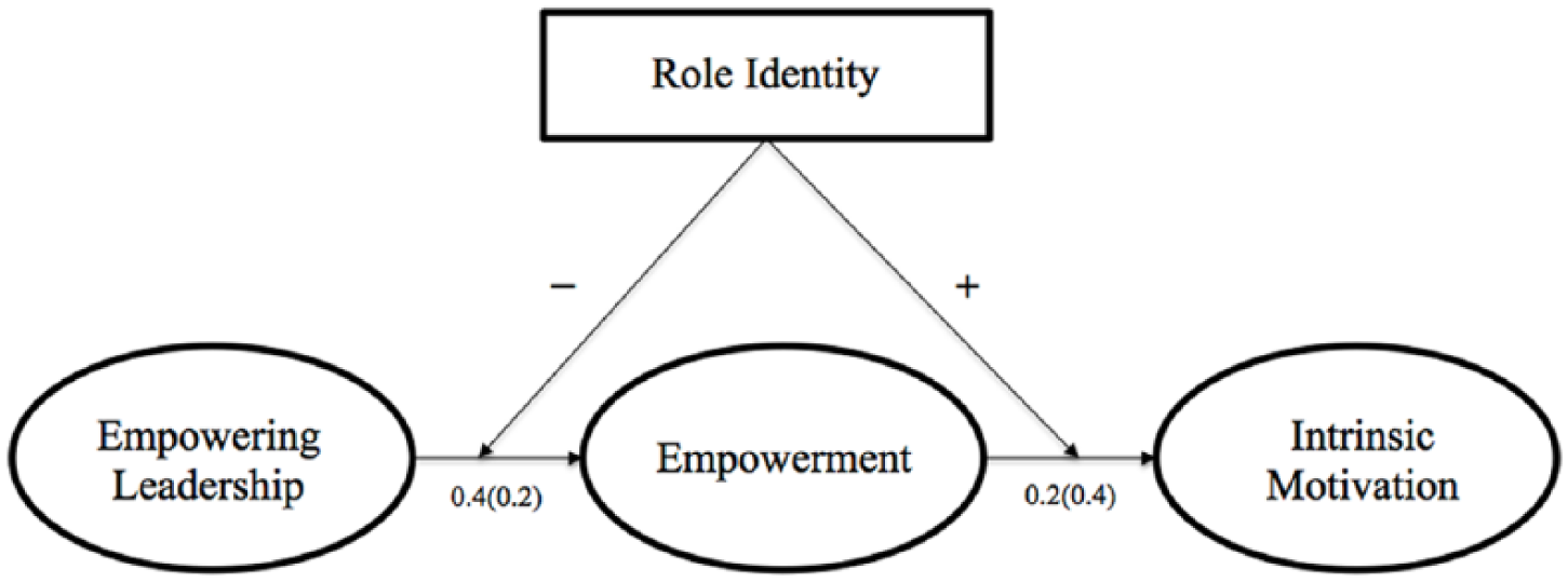
Example of Conditional Indirect Effects Model Containing Restricted Variance Interactions

When role identity is high (i.e., strength is low), the a and b coefficients in the indirect effect are 0.4 and 0.2, for an indirect effect of 0.08. When role identity is low, the coefficients are 0.2 and 0.4, resulting in the same indirect effect. Put another way, the compressing effect of role identity in one relationship is canceled out by its compressing effect in the other, leaving the indirect effect unchanged across levels of the moderator.

As another example, consider the role of family logics in family-intensive models of governance by Miller, LeBreton-Miller, Amore, Minichilli, and Corbetta (2017). In this model, family logics (i.e., community assumptions and values regarding centrality of family) lead to more family-intensive models of governance (i.e., family businesses continue to be run by family members: Hypothesis 1); logics also moderate the relationship between family-intensive models of governance and firm performance (Hypothesis 2) because family logics make it difficult to base hiring and promotion decisions on competence. Thus, X causes M and moderates the relationship between M and Y because of its effect on Z. RV reasoning provides a simpler explanation.

In communities with strong family logics, family governance is more or less mandatory. Thus, top management is made up of family members regardless of their competence. “Familiness” of top management is high regardless of competence or anything else. In communities with weak family logics, “familiness” is not constrained to be high and is free to vary. It is also free to covary with competence of family members. The relationship between competence of family members and familiness is positive in communities with weak family logics, but it is near zero in communities with strong logics because familiness has so little variance.

In this model, familiness is a mediator between family competence and firm performance. Thus, familiness is the DV in the first stage and the predictor in the second stage. Just as family logics reduce the competence-familiness relationship by compressing the variance of familiness, so must logics strengthen the positive relationship between familiness and firm performance by compressing variance on familiness. As a result, the indirect effect of family competence and firm performance is the same regardless of family logics. We found many examples of RV interactions stemming from mediator compression but none in which this canceling-out effect was appreciated.

Distinguishing RV interactions from range restriction

It is important to distinguish between RV interactions and issues relating to restriction of range. Such issues have been a common part of the personnel selection literature and are increasingly common in other areas of management (Aguinis et al., 2017). The term restriction of range is used to describe a situation in which there is direct or indirect selection on one of the variables in a system. The result is truncation, which biases parameter estimates and generally increases the probability of Type II errors. Consider the examples in Sackett and Yang (2000). Figures 1b and 1d from their article represent the classic examples. In Figure 1b, because of selection on X, the sample simply does not contain any of the people who scored below a certain point on X. Figure 1d contains indirect restriction such that the probability of a person being excluded increases as a function of Z. Similar patterns can be found in strategy research because firms or joint ventures that perform very poorly are often omitted from common data sources (Bergh et al., 2014).

In RV phenomena, cases are not excluded. Rather, scores on a particular variable are compressed in a particular direction as a function of the moderator. The difference is best understood with the following description of truncation effects from Sackett and Yang (2000):

The larger reduction in sample covariance (the numerator in the formula for a correlation) relative to the reduction in a multiplicative term of two sample standard deviations s_x and s_y (the denominator in the formula for a correlation) leads to a reduction [italics added] in the sample correlation from .50 to .33. (p. 112)

By contrast, the compression in an RV phenomenon creates proportional changes in the numerator and the denominator of the correlation formula, leaving r and β unchanged.

However, Sackett and Yang (2000) also note that selection/truncation on X has no effect on the unstandardized weight b. But as we showed earlier, the compression in an RV phenomenon does affect b, and this is true regardless of whether the compression is on X or Y. The reason is that the denominator in the formula for b is s²_x, whereas the denominator of the formula for β is s_xs_y. As can be seen, the arguments needed to support RV interactions are very different from those needed to support a range restriction hypothesis because the latter involves exclusion of cases whereas the former involves reduction in plausibility of values of certain variables as a function of the moderator.

A related issue has to do with the distinction between differential prediction and differential validity. Differential prediction refers to unstandardized slope differences and is appropriately tested by moderated multiple regression or latent moderated structural equation modeling (LMS; Klein & Moosbrugger, 2000). Evidence for differential prediction comes from a comparison of unstandardized regression coefficients at different levels of the moderator. Differential validity refers to correlational differences between the predictor and outcome (i.e., the percentage of variance in Y that is explained by X changes as a function of Z) and is usually tested by comparing correlation coefficients (or beta weights) across subgroups (Andersson et al., 2014; Arnold, 1982; Carte & Russell, 2003).

RV interactions represent a form of differential prediction. Standardized indices, such as correlation coefficients and beta weights, are not affected by compression of values, because they are based on variables with the same standard deviation. Put another way, RV affects covariance (the numerator of the correlation formula) and the product of standard deviations (the denominator of the correlation formula) proportionally, so standardized indices of covariation are unaffected. However, unstandardized indices, such as unstandardized regression coefficients and covariances, are influenced by compression of values. Thus, one can find an interaction effect due to compression of values even when there are no differences in correlations.

Consider once again the examples in Tables 1 and 2. As we showed earlier, the compression of fear expression scores in Table 2 results in covariances and unstandardized weights that differ, and this produces the interaction in Table 3. The correlation, however, is the same in the two subsamples. Arnold (1982) demonstrated how standardization of variables can mask interaction effects by using as an example the relationship between a rectangle’s length and area. Obviously, the area of a rectangle is the product of its length and width; that is, they interact to determine area. Given two groups of rectangles of equal average length but different widths, if we regressed area onto length in each group, we would find different unstandardized weights and, therefore, a Length × Width interaction. Yet the correlation between length and area is the same (r = 1) in both groups, making it appear as though the relationship between length and area does not depend on width. Arnold stated that

the fact that area is equal to the product of length and width causes σ_y to vary for groups of rectangles of differing widths, and these σ_y differences result in the necessary b differences which signal the fact that the form of the relationship between length and area is conditional upon width. (p. 148)

The primary implication of all of this is that although the typical tests for interaction—such as moderated regression, LMS, or even multiple-groups analysis with unstandardized values—will detect an RV interaction, a comparison of correlations or standardized weights will not.

Issues in Testing and Reporting RV Interactions

The options for testing interaction effects generally depend on whether the moderator variable is categorical or continuous. When the moderator is categorical, the relationship between X and Y can be tested at the different levels (or within different groups) of Z in a multiple-groups analysis. When the moderator is continuous, this option no longer exists without losing information. Interaction effects are generally tested by forming products of predictors and examining the relationship between the partialed product and Y. In multiple-groups analysis, an interaction effect is supported when the path linking X and Y is substantially different across the different Z groups. For continuous moderating variables, an interaction hypothesis is supported when the coefficient attached to the product term is substantial, showing that the product term contributes to the prediction of Y over and above the additive model. An increasingly common alternative is LMS (Klein & Moosbrugger, 2000), which estimates the relationship between the moderator and the X-Y slope without the use of products. Regardless of the analysis approach, the form or pattern of an interaction is demonstrated by reporting or plotting the X-Y relationship across different levels of Z (Cohen et al., 2003, p. 268).

The RV interaction is, above all else, an interaction. Tests of RV interactions begin with the same steps as do other sorts of interactions. As with most tests of interaction, one might begin with a moderated regression, looking for a substantial weight for the partialed product. If one were testing a cross-level model, one might instead regress level k slopes onto a level k + 1 moderator. If one were using LMS, one might conduct the log-likelihood difference test between the linear and interaction models. There are, however, some additional requirements and some issues that are peculiar to the testing of RV interactions. In an RV interaction, the reason for the pattern is that certain values of one variable are implausible at certain combinations of values of another variable and the moderator. Thus, it must be demonstrated that variance in the restricted variable differs across levels of the other variable and/or moderator as hypothesized. To confirm the hypothesized RV pattern, one must look at all the coefficients (including the intercept) in the moderated regression equation on centered variables, and one must also determine the actual pattern of heteroscedasticity as we explain later.

RV-specific follow-ups

If one hypothesizes an RV interaction, then there are some specific follow-up analyses that are needed. Once the presence of an interaction has been determined, one must discover whether the interaction is due to compression as hypothesized.³

Let us return to Ilies et al. (2006) for an example. Agreeableness moderates the relationship between positive affect and OCB such that the relationship is weaker for those high in agreeableness. The RV explanation is that those who are high in agreeableness are uniformly high in OCB. As a result, positive affect is less predictive of OCB when agreeableness is high. Our analyses must of course show the appropriate Affect × Agreeableness interaction. To support the RV hypothesis, they must also show less OCB variance when agreeableness is high than when low.

As is usually the case with interactions, plots can be useful. As mentioned earlier, Figure 4 contains a scatterplot that would be consistent with Ilies et al. (2006), with compression of Y when Z (or X) is high. Figures 11 and 12 also depict interactions that are consistent with the notion that the relationship between OCB and one exogenous variable is weaker when the other exogenous variable is high, but neither is consistent with this specific RV argument because the compression occurs in the wrong place. In Figure 11, the compression occurs in the middle of the agreeableness range. In Figure 12, it occurs at the beginning.

Figure 11

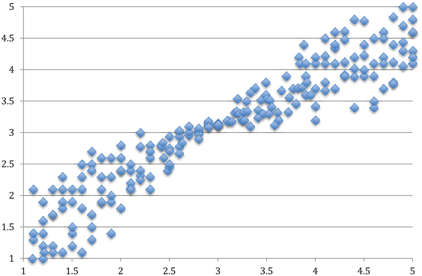
Compression at Moderate Levels

Figure 12

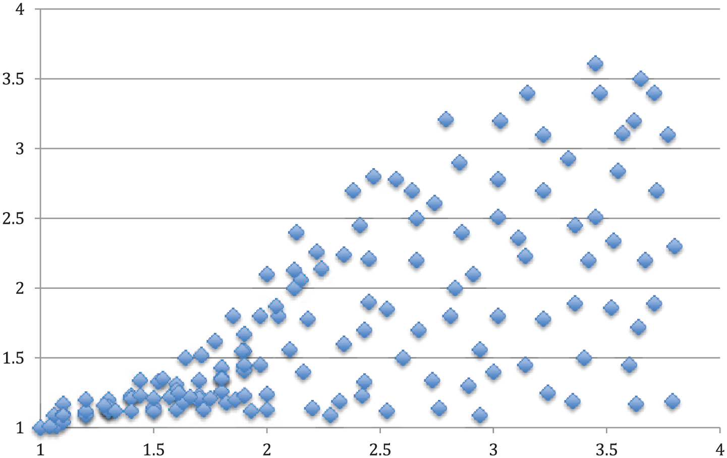
Compression at Low Levels

In addition, it is useful to demonstrate that variance does in fact differ substantially across levels of the moderator (or the predictor). The most common tests for equality of variances are Bartlett’s test (1937) and Levene’s test (1960), the latter of which was developed to be less arduous and less sensitive to departures from normality. Because Bartlett’s test is less useful when raw data are available, we focus our attention on Levene and its common extension, Brown-Forsythe. Levene’s test is a one-way fixed effects analysis of variance on within-group absolute deviations (Glass, 1966). Thus, it is an F test against the null hypothesis:

H_{0} : σ_{1}^{2} = σ_{2}^{2} = \dots σ_{j}^{2}

for j groups on [(j − 1), (n₁ − 1 + n₂ − 1 + . . . n_j − 1)] degrees of freedom. Brown and Forsythe (1974) found Levene’s test to be sensitive to departures from normality and developed a more robust procedure based on deviations from the median rather than the mean. Levene’s test is available in most major statistical software packages. Unfortunately, what is labeled Brown-Forsythe in most packages (e.g., SPSS, R) is not the test for variance differences but is instead a robust test of mean differences. (For detailed illustrations of these procedures with various software packages, go to www.josecortina.com.) Using the data from Tables 1 and 2 as an example, we can determine whether the strength of the situation compresses variance on expressions of fear by running Levene’s and Brown-Forsythe tests. When we do this, both tests are significant (Levene’s F = 5.281, p = .03; Brown-Forsythe F = 4.81, p = .04), thus allowing us to reject the null hypothesis that variance is equal across these two levels of the moderator. The difference in variances is in the anticipated direction, with less variance in the “strong” situation.

For continuous moderators, there are two options. The first is to categorize the moderator and conduct the same tests described in the previous paragraph. Although categorizing loses information, this can be a pragmatic solution. One must simply ensure that there are enough groups to detect any likely nonlinearities in the relationship between the moderator and variance (see Figure 11 for an example). In the (likely) absence of such nonlinearity, one might simply select cases in the bottom and top quartiles on the moderator and compare the two variances with Levene and/or Brown-Forsythe.

Alternatively, one might leave the moderator intact and conduct what amounts to a test for homoscedasticity. One of the assumptions of the ordinary least squares estimator is that, for any set of values of the predictors, the variance of errors is constant, which is to say, there is homoscedasticity. In testing an RV interaction, our interest is not in the variance of errors but in the variance of the compressed variable itself. If the compressed variable is the DV, then the standard test for constant error variances actually gives us what we need. To see this, one must first remember that there is no mathematical distinction between the “predictor” and the “moderator” in an interaction model—what is true of the moderator is true of the predictor. Next, one must realize that the standard test for homoscedasticity is equivalent to a test of the relationship between the predictor and the variance of the DV (for a concise explanation of this fact, see Berry, 1993, p. 73). These two facts lead to the conclusion that the test for homoscedasticity provides the test for DV compression that we need.

The recommended test is that developed by Breusch and Pagan (1979). The first step in the Breusch-Pagan test is simply to regress the outcome onto the moderator with the goal of generating a column of residuals ( $Y - \hat{Y}$ values). The residuals are squared, and the squared residuals are regressed back onto the moderator. A positive regression weight suggests that variance increases as the moderator increases, with compression of Y values at the low end of the moderator scale. Finally, the R² value from this last regression is multiplied by the sample size. This product is chi-square distributed with degrees of freedom equal to the number of predictors. A significant chi-square suggests that variance is not constant across values of the moderator (see the illustrations at www.josecortina.com).

If the compression is in the IV, then the equation can simply be turned around such that the IV is regressed onto the moderator, with the same procedure being otherwise followed.

Discussion and Conclusion

The purpose of this article was to explore the nature of interactions that exist because certain values of one or more variables in a system are unlikely when another variable in the system takes on certain values. The result is compression, and this compression creates an interaction effect: the RV interaction.

We explain the nature of RV interaction arguments and make the case that such arguments are relatively easy to make, thus simplifying a justification process with which many struggle. To justify an RV interaction hypothesis, one need only explain (a) that certain values of one or more variables in a system are implausible at certain levels of a moderator, thus restricting the variance of that variable; (b) that the same variable has full variance at other levels of the moderator; and (c) that these differences in variance create particular differences in relationships with other variables.

We then describe the various forms that such interactions can take. We show that whereas restriction on the DV tends to suppress its relationship with an IV, restriction on the IV has the opposite effect. We also discuss RV interactions in the context of mediation models, quadratic models, and higher-order interaction models. We illustrate these forms with examples from the published literature and show how a given interaction form could be justified with a particular RV argument.

Finally, we discuss some of the empirical evidentiary requirements that are unique to RV interactions. Essentially, one must show that variance compression occurs where it is supposed to and nowhere else. Descriptions, examples, and requirements are summarized in Table 5.

Table 5

Descriptions, Examples, and Evidentiary Requirements for the Different Types of RV Interactions

RV interaction	Explanation	Example	Testing
DV compression buffering interactions	The moderator Z compresses the variance of Y in such a way that it acts as a buffer against the effects of X, reducing the importance of X for Y. The X and Z effects are of opposite sign.	Use of an interim CEO is negatively related to audience reactions, but sudden CEO departure acts as a buffer by making extremely negative reactions unlikely, thus reducing the negative relationship between use of interim CEO and reactions (Marcel Cowen, & Ballinger, 2017).	A test for moderation is conducted, and the expected pattern is one in which the two main effects are in the opposite direction. Moreover, it must be demonstrated that DV variance changes as a function of the moderator in the expected direction. In this example, the Brown-Forsythe test should show that variance in audience reactions is significantly smaller for firms from which the CEO departed suddenly than for firms from which the CEO departed gradually.
DV compression interference interactions	The moderator Z compresses the variance of Y in such a way that it interferes with the effects of X, thus reducing the importance of X for Y. The X and Z effects are of the same sign, but the interaction is in the opposite direction. If the main effects are positive, then values of the outcome are restricted to high levels when the moderator is high. If the main effects are negative, then the opposite is true.	Agreeableness “interferes” with positive affect such that positive affect is not necessary for OCBs among highly agreeable people, for whom OCBs are high regardless of affect (Ilies, Scott, & Judge, 2006).	A test for moderation is conducted, and the expected pattern is one in which the two main effects are in the same direction and the interaction is in the opposite direction. Moreover, the Breusch-Pagan test should show that variance in OCB decreases as a function of agreeableness.
IV compression interactions	The moderator Z compresses the variance of X. This strengthens the relationship between X and Y by reducing the numerator of b to a lesser extent than the denominator of b. In IV compression interactions, the variability in Y does not change as a constant function of X. Instead, variability increases until the (compressed) limits of X are reached, and then variability in Y drops back down. Compression on the IV instead of the DV results in a different magnitude of interaction; however, the change in the standard error of the product is proportional, resulting in the same t and p values as would be found with compression on the DV. However, compression on the IV makes the X-Y slope steeper rather than shallower.	For job applicants, self-reported personality scores are compressed upward (e.g., higher conscientiousness), whereas for nonapplicants, this is not the case (Schmit & Ryan, 1993). This compression would result in a stronger conscientiousness-GPA relationship for applicants than for nonapplicants.	A test for moderation is conducted, and the expected pattern is one in which the X-Y slope is steeper (i.e., either more positive or more negative) when Z is at its stronger levels. Moreover, variance in self-reported conscientiousness should be smaller for applicants than for nonapplicants.
Compression on IV and DV	The moderator Z compresses the variance of both X and Y. If compression is equal, then there should be no XZ interaction. An interaction will exist to the degree that the amount of compression differs.	Ozer (2011) implied that a lack of autonomy would limit both OCB (X) and TMX (Y). If a lack of autonomy created the same amount of compression on both OCB and TMX, then there should be no OCB × Autonomy interaction.	If equal compression is expected, then the interaction need not be tested at all. One need only examine the effect of Z on the variances of X and Y. If unequal compression is expected, then an interaction would be expected. Regardless, the appropriate test of variance differences would be conducted on both variables.
Three-way RV interactions	The moderator Z compresses variance on the DV in a two-way interaction. This compression on the DV will tend to weaken all relationships, both additive and multiplicative.	The interference interaction hypothesized by Ilies et al. might itself be interfered with if a unit-level variable compressed variance in OCB. OCB might be uniformly high in units with strong norms for citizenship. For units with weak norms, OCB might be uniformly high for those high in agreeableness but vary as a function of positive affect for those low in agreeableness.	A test for three-way interaction is conducted, and the expected pattern is one in which, when the overriding variable (e.g., unit norms) is weak, the lower-level IVs demonstrate their hypothesized interaction pattern. When the overriding variable is strong, most or all of the lower-level relationships are washed out. Moreover, OCB variance, within and between person, should be low in units with strong OCB norms. In units with weak norms, within-person variance in OCB should be low for agreeable people.
Nonlinear RV effects and interactions	If an omitted moderator Z produces a ceiling or floor effect, the result will be a nonlinear relationship between X and Y due to changes in the variance of Y. If the ceiling/floor exists for some people but not for others, then a nonlinear interaction is expected.	Ceiling effect refers to a phenomenon in which higher scores in a range are implausible. X and Y might be positively related, but if there is a ceiling for Y, then a diminishing-returns pattern will emerge such that higher X is associated with higher Y until the ceiling on Y is reached. Beyond that point, additional X is not associated with higher Y. The ceiling effect might exist for some people (e.g., women) but not for others. This would be the glass ceiling.	A test for a quadratic effect is tested, and the expected pattern would be concave downward or upward depending on whether there is a ceiling or a floor. If this curvilinearity is expected for some levels of a second predictor but not others (e.g., for women but not men), then a three-way (X × X × Z) interaction is tested. Moreover, it must be demonstrated that DV variance changes as a function of the DV itself (or the IV as it amounts to the same thing). If there is a moderator of this relationship, then it must also be demonstrated that this variance function changes as a function of the moderator. Using the glass ceiling as an example, it must be demonstrated that promotion variance decreases as a person climbs the hierarchy and that promotion variance remains constant for men.
Conditional indirect effects with RV interactions	If moderator Z compresses variance on a variable in a CIE model, the effect depends on where in the model the compression occurs. Compression on X will strengthen the direct and indirect effects of X on Y. Compression on Y will weaken both effects. Compression on M will weaken the X-M linkage but strengthen the M-Y linkage.	Zhang and Bartol (2010) hypothesized a model in which empowering leadership increases empowerment, which in turn increases motivation. If role identity compresses variance in empowerment, then increases in role identity should weaken the empowering leadership-empowerment relationship but strengthen the empowerment-motivation relationship.	A test for a conditional indirect effect is conducted such that the magnitude or direction of the relevant linkages is shown to vary as a function of the moderator, as is the indirect effect. Moreover, variance in empowerment should be low when role identity is low, thus weakening the first stage of the CIE but strengthening the second stage.

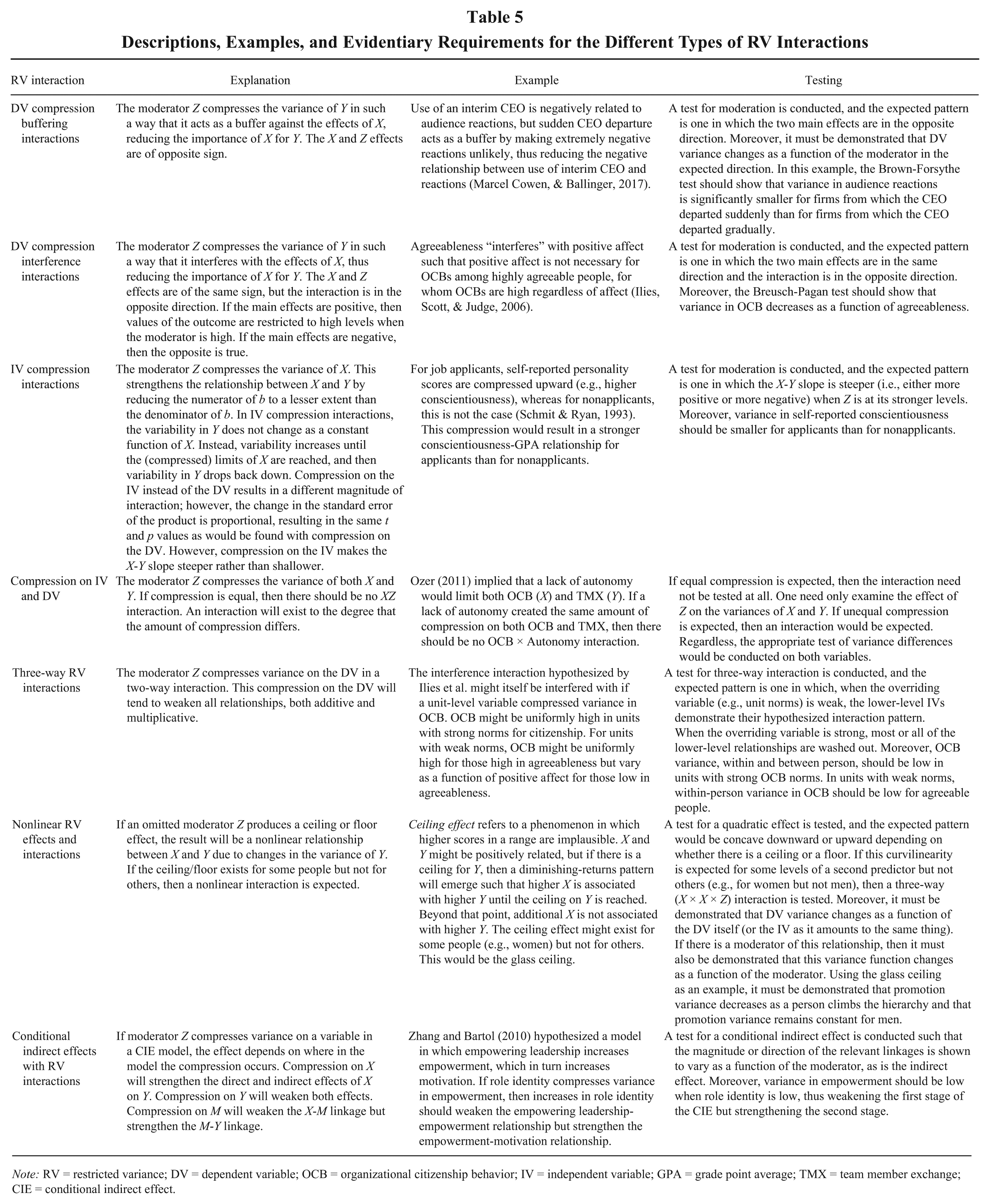
Note: RV = restricted variance; DV = dependent variable; OCB = organizational citizenship behavior; IV = independent variable; GPA = grade point average; TMX = team member exchange; CIE = conditional indirect effect.

Contributions to Research

Our article makes several important contributions. First, recent work has called for more appropriate theorizing of interaction effects, bemoaning that interaction effects are often not properly or inaccurately justified. More accurate theorizing comes from a better understanding of how interaction effects work. In the current article, we demonstrate how researchers can use RV logic and patterns to theorize about and test interaction effects. By offering concrete examples for appropriate theoretical justification, we hope to further theoretical development in a range of research that involves interaction hypotheses.

Furthermore, we explain how this class of interaction effects should be tested to determine whether findings are in fact consistent with underlying theory. We show how interpretations of prominent findings in the literature could be augmented with RV arguments and with exploration of variance patterns in the data.

Identifying the precise dynamics of interaction effects may also have important practical implications. When we test specific RV models, we can better understand which conditions allow or exacerbate an effect or issue (e.g., stereotyping or discriminatory hiring and promotion) and which conditions may neutralize it and why. Understanding the role of variance restriction could open up new avenues for research that illuminates how contextual factors can be employed to evoke desirable or suppress undesirable behaviors. At the same time, this knowledge can allow practitioners to create contexts that facilitate organizational interventions.

Finally, we hope that providing this introduction of RV interactions instigates a discussion of the importance of distinguishing different types of moderator models, their related theoretical rationales, and their testing. It seems that there is still much work to be done.

Footnotes

Acknowledgements

We wish to express our gratitude to Ernest O’Boyle and two anonymous reviewers for their insightful comments. Work on the article was supported by the University of Melbourne’s Faculty of Business and Economics and by the University of Sydney Business School.

Notes

References

Aguinis

1995. Statistical power problems with moderated multiple regression in management research. Journal of Management, 21: 1141-1158.

Aguinis

Beaty

J. C.

Boik

R. J.

Pierce

C. A.

2005. Effect size and power in assessing moderating effects of categorical variables using multiple regression: A 30-year review. Journal of Applied Psychology, 90: 94-107.

Aguinis

Edwards

J. R.

Bradley

K. J.

2017. Improving our understanding of moderation and mediation in strategic management research. Organizational Research Methods, 20: 665-685.

Andersson

Cuervo-Cazurra

Nielsen

B. B.

2014. From the editors: Explaining interaction effects within and across levels of analysis. Journal of International Business Studies, 45: 1063-1071.

Arnold

H. J.

1982. Moderator variables: A clarification of conceptual, analytic, and psychometric issues. Organizational Behavior and Human Performance, 29: 143-174.

Bartlett

M. S.

1937. Properties of sufficiency and statistical tests. Proceedings of the Royal Society of London: Series A, Mathematical and Physical Sciences, 160: 268-282.

Bergh

D. D.

Aguinis

Heavey

Ketchen

D. J.

Boyd

B. K.

Joo

2014. Using meta-analytic structural equation modeling to advance strategic management research: Guidelines and an empirical illustration via the strategic leadership-performance relationship. Strategic Management Journal, 37: 477-497.

Berry

W. D.

1993. Understanding regression assumptions. Newbury Park, CA: Sage.

Breusch

T. S.

Pagan

A. R.

1979. A simple test for heteroskedasticity and random coefficient variation. Econometrica, 47: 1287-1294

10.

Brown

M. B.

Forsythe

A. B.

1974. Robust tests for the equality of variances. Journal of the American Statistical Association, 69: 364-367.

11.

Carte

T. A.

Russell

C. J.

2003. In pursuit of moderation: Nine common errors and their solutions. MIS Quarterly, 27: 479-501.

12.

Chowdhury

S. K.

Endres

M. L.

2010. The impact of client variability on nurses’ occupational strain and injury: Cross-level moderation by safety climate. Academy of Management Journal, 53: 182-198.

13.

Cohen

West

S. G.

Aiken

L. S.

2003. Applied multiple regression/correlation analysis for the behavioral sciences. Mahwah, NJ: Erlbaum.

14.

Cortina

J. M.

1993. Interaction, nonlinearity, and multicollinearity: Implications for multiple regression. Journal of Management, 19: 915-922.

15.

Cortina

J. M.

2003. Apples and oranges (and pears, oh my!): The search for moderators in meta-analysis. Organizational Research Methods, 6: 415-439.

16.

Cortina

J. M.

Köhler

Nielsen

B. B.

2015. Restriction of variance interaction effects and their importance for international business research. Journal of International Business Studies, 46: 879-885.

17.

Cotter

D. A.

Hermsen

J. M.

Ovadia

Vanneman

2001. The glass ceiling effect. Social Forces, 80: 655-681.

18.

Edwards

J. R.

Lambert

L. S.

2007. Methods for integrating moderation and mediation: A general analytical framework using moderated path analysis. Psychological Methods, 12: 1-22.

19.

Frazier

P. A.

Tix

A. P.

Barron

K. E.

2004. Testing moderator and mediator effects in counseling psychology research. Journal of Counseling Psychology, 51: 115.

20.

Glass

G. V.

1966. Testing homogeneity of variances. American Educational Research Journal, 3: 187-190.

21.

Holland

S. J.

Shore

D. B.

Cortina

J. M.

2017. Review and recommendations for integrating mediation and moderation. Organizational Research Methods, 20: 686-720.

22.

Ilies

Scott

B. A.

Judge

T. A.

2006. The interactive effects of personal traits and experienced states on intraindividual patterns of citizenship behavior. Academy of Management Journal, 49: 561-575.

23.

King

E. B.

Ahmad

A. S.

2010. An experimental field study of interpersonal discrimination toward Muslim job applicants. Personnel Psychology, 63: 881-906.

24.

Klein

Moosbrugger

2000. Maximum likelihood estimation of latent interaction effects with the LMS method. Psychometrika, 65: 457-474.

25.

Levene

1960. Robust tests for equality of variances. Contributions to Probability and Statistics, 1: 278-292.

26.

Liu

Wright

Filatotchev

2014. International experience and FDI location choices of Chinese firms: The moderating effects of home country government support and host country institutions. Journal of International Business Studies, 45: 428-449.

27.

Lyness

K. S.

Heilman

M. E.

2006. When fit is fundamental: Performance evaluations and promotions of upper-level female and male managers. Journal of Applied Psychology, 91: 777.

28.

Marcel

J. J.

Cowen

A. P.

Ballinger

G. A.

2017. Are disruptive CEO successions viewed as a governance lapse? Evidence from board turnover. Journal of Management, 43: 1313-1334.

29.

Meyer

R. D.

Dalal

R. S.

Hermida

2010. A review and synthesis of situational strength in the organizational sciences. Journal of Management, 36: 121-140.

30.

Miller

LeBreton-Miller

Amore

M. D.

Minichilli

Corbetta

2017. Institutional logics, family firm governance, and performance. Journal of Business Venturing, 32: 674-693.

31.

Mischel

1973. Toward a cognitive social learning reconceptualization of personality. Psychological Review, 80: 252-283.

32.

Murphy

K. R.

Russell

C. J.

2017. Mend it or end it: Redirecting the search for interactions in the organizational sciences. Organizational Research Methods, 20: 549-573.

33.

Ozer

2011. A moderated mediation model of the relationship between organizational citizenship behaviors and job performance. Journal of Applied Psychology, 96: 1328-1336.

34.

Preacher

K. J.

Rucker

D. D.

Hayes

A. F.

2007. Addressing moderated mediation hypotheses: Theory, methods, and prescriptions. Multivariate Behavioral Research, 42: 185-227.

35.

Sackett

P. R.

Yang

2000. Correction for range restriction: An expanded typology. Journal of Applied Psychology, 85: 112-118.

36.

Schmit

M. J.

Ryan

A. M.

1993. The Big Five in personnel selection: Factor structure in applicant and nonapplicant populations. Journal of Applied Psychology, 78: 966.

37.

Schmit

M. J.

Ryan

A. M.

Stierwalt

S. L.

Powell

A. B.

1995. Frame-of-reference effects on personality scale scores and criterion-related validity. Journal of Applied Psychology, 80: 607.

38.

Stone

E. F.

Hollenbeck

J. R.

1984. Some issues associated with the use of moderated regression. Organizational Behavior and Human Performance, 34: 195-213.

39.

Wang

Zhang

McArdle

J. J.

Salthouse

T. A.

2008. Investigating ceiling effects in longitudinal data analysis. Multivariate Behavioral Research, 43: 476-496.

40.

Zhang

Bartol

K. M.

2010. Linking empowering leadership and employee creativity: The influence of psychological empowerment, intrinsic motivation, and creative process engagement. Academy of Management Journal, 53: 107-128.

41.

Zheng

Singh

K. W.

Chung

2017. Ties to unbind: Political ties and firm sell-offs during institutional transition. Journal of Management, 43: 2005-2036.