Pay Volatility and Employee Turnover in the Trucking Industry

Abstract

Many organizations have turned to “just-in-time” pay systems to manage fluctuations in demand for products and services. For example, the trucking industry commonly pays truck drivers by the mile, and retail organizations fluctuate hours available to work to align with holiday demand. Based on the Unfolding Model of Turnover, we propose that the pay volatility, that is, fluctuations in individual pay over time, created by such systems create shocks that initiate thoughts of leaving the organization. We propose that these thoughts increase turnover likelihood. We also propose that pay level and pay trajectory moderate the pay volatility and turnover relationship. Based on a large dataset containing information on objective pay and turnover for truck drivers over a period of 34 weeks, the results of this study support the role of pay volatility, pay level, and pay trajectory in affecting voluntary turnover. Specifically, the results show that all three factors predict turnover likelihood and that pay volatility and pay level interact to predict turnover likelihood. The findings indicate that pay volatility has organizational downsides due to its effects on employee turnover in addition to its known upsides (i.e., flexibility).

Keywords

compensation bonuses benefits turnover survival analysis research methods

One aspect of pay system design involves who bears the risk of fluctuations in product and service demands. Organizations appear to prefer pushing such risk to employees (Aspen Institute, 2016). For example, when organizations implement individual-level commission pay systems, employees bear the risk of poor sales affecting their paycheck since organizations’ payroll expenses fluctuate with product sales. Or when pay varies by the number of hours worked, employees’ paychecks are at the mercy of scheduling. Food service employees may see increases in hours during high demand weeks (e.g., finals week in college towns), while retail workers may experience swings in paychecks as managers deal with scheduling issues related to product demand, employee vacations, and sick leave, among the many influential factors. In another context, trucking, pay is typically based on miles driven, so drivers can see significant fluctuations in pay from week to week as their driving assignments vary. In each of these cases, the organization benefits by only paying for output or the work needed, while employees may experience a roller coaster of fluctuations from paycheck to paycheck.

These fluctuations in pay represent pay volatility, which is at least partly driven by organizational policies and practices. As described above, some pay volatility can be expected in organizations with employment policies that focus on paying only for output or time spent at work. This allows employers to better manage payroll costs, but it leaves employees with some level of unpredictability in their paychecks. On the one hand, pay volatility may have some benefits for the employer, allowing flexibility in costs and lower risk. On the other hand, employees are often risk averse and indicate preferences for stability in their spending ability (Mas & Pallais, 2017). Given such reported preferences, we believe there are unexplored downsides for employers associated with high levels of pay volatility.

This study explores the relationship between paycheck-to-paycheck volatility and one potentially negative consequence for employers—employee voluntary turnover. Voluntary, that is, employee-initiated, turnover is an important outcome of pay volatility for several reasons. One, voluntary turnover is of critical concern to many organizations and is associated with increased costs and lower productivity (Allen, Bryant, & Vardaman, 2010; Hom, Allen, & Griffeth, 2020). Two, high voluntary turnover rates have been of significant concern in the industry where this study is conducted (i.e., trucking), and voluntary turnover is viewed as a highly undesirable outcome in this industry (Whitaker, 2010). If pay volatility is found to be a significant predictor of turnover, trucking organizations that can find a way to better manage this volatility may find a competitive advantage in their compensation strategy without having to substantially increase actual pay levels. Three, voluntary turnover represents an objective outcome influenced by pay (Rubenstein, Eberly, Lee, & Mitchell, 2018; Shaw, Delery, Jenkins, & Gupta, 1998). It has been asserted that there is a substantial difference between “what people say and what they do” in regard to pay (Rynes, Gerhart, & Minette, 2004: 381), so it is especially valuable to measure objective behavioral outcomes in response to compensation. Of greatest relevance to organizations grappling with compensation issues is understanding the behavioral outcomes of compensation, with turnover representing one of the most critical of these outcomes.

We employ and extend the Unfolding Model of Turnover (Lee & Mitchell, 1994) to predict the effects of pay volatility. We propose that when recurring paychecks are studied in context of pay over time, changes in pay have the potential to be perceived as “shocks” (i.e., jarring events that initiate thoughts of organizational exit; Lee & Mitchell, 1994) that will increase the likelihood of voluntary employee turnover. In particular, we propose that for employees whose paychecks vary over time (e.g., they are not on a fixed salary), each weekly paycheck has the potential to create a shock, though this will not always occur. Lee and Mitchell (1994: 60) stated that a shock generates “information or has meaning about a person’s job,” is “sufficiently jarring that it cannot be ignored,” and produces “job-related deliberations that involve the prospect of leaving a job.” Given this definition, in order to understand when a shock will occur in any type of recurring event, it is necessary to view the event in the context of the recurring events over time. Applying this to pay indicates that when pay volatility is high, large deviations occur across time and thus a paycheck in that time period has greater potential to be perceived as a shock. When pay volatility is low, there is little about each paycheck that will draw an employee’s attention, and thus, paychecks during more stable strings of recurring paychecks are unlikely to be perceived as shocks. Thus, for the study of nonfixed base pay in turnover, our research demonstrates that paychecks must be studied in context of recurring pay dynamics. We examine the relationship of pay volatility over a period of 4 weeks and subsequent voluntary turnover using a dataset containing 34 weeks of information on weekly pay levels and voluntary turnover for over 14,000 truck drivers in a single trucking company.

Our investigation of pay volatility and voluntary turnover makes several contributions. First, we examine a form of pay change (i.e., intrayear pay volatility) that is a rarely studied yet important phenomenon in organizations. This approach addresses a critical oversight of current compensation research (e.g., Gupta & Shaw, 2014; Shaw, 2014) with theoretical implications and, at the same time, addresses an issue with important policy implications (Aspen Institute, 2016). Many workers in the modern economy experience fluctuations in pay from month to month or even week to week. For example, truck drivers—the focus of this study—are usually paid by the number of miles driven, and many hourly workers work overtime some days and are sent home early on other days. This leads to weekly, semimonthly, or monthly fluctuations in pay as employers shift risk associated with product or service demand to employees; however, we know little about how employees respond to a combination of upward and downward changes in compensation. Research addressing pay dynamics over time is rare. The primary stream of compensation research that has addressed pay changes is the just noticeable difference (JND) literature, which has studied when increases in pay are “noticeable” (i.e., elicit an affective response). Studies report that changes in pay are only noticed when they reach a certain threshold (between 5% and 8%; Mitra, Gupta, & Jenkins, 1997; Mitra, Tenhiälä, & Shaw, 2016). This research would indicate that higher pay volatility is likely to be more noticeable than low volatility. Connecting this noticeability to the Unfolding Model of Turnover, we argue higher pay volatility is more likely to be “jarring” to employees. Our research extends this literature by studying the effects of fluctuations, both increases and decreases in pay, over time, and connecting these ideas to turnover outcomes. We assess behavioral outcomes, rather than intentions or affective responses, of such changes. Prior work of pay changes has been limited both conceptually and empirically to upward changes in pay and nonbehavioral responses. Our approach contributes to the compensation literature by indicating that pay changes are “shocks” that lead to behavioral responses.

Practically, employers have been identified as the best positioned to address issues of income volatility (i.e., fluctuation in income, which could include pay from multiple employers, government subsidies, or other payments) in society due to their influence on pay volatility, yet few experts believe employers are likely to take action to reduce such volatility (Mitchell, 2017). Pay volatility involves shifting risk to employees, and without clear evidence that reducing volatility has positive outcomes for the employer, there is little incentive for organizations to change volatility-creating practices. Studies, like ours, that provide a better understanding of the outcomes of volatility can inform employers in their pay system design.

Second, we contribute to the compensation literature by examining a legitimate, though non-performance-based, driver of pay. Much of the pay literature emphasizes that explained and legitimate pay differences will lead to positive, functional outcomes and illegitimate, unexplained pay difference will lead to negative, dysfunctional outcomes (Downes & Choi, 2014; Trevor, Reilly, & Gerhart, 2012). At times, research on pay has conflated performance basis and legitimacy. Studies of pay-for-performance, one of many legitimate pay bases, address controllable, performance-based differences; our study addresses a context where pay differences have a legitimate cause, but the cause is low on controllability for the employee. Thus, we theorize that because the legitimate pay changes in our study are not controllable by the employee and occur in both positive and negative directions, such legitimate pay changes can be shocking, and undesirable outcomes may follow. This research brings into question the assumption that legitimate, explained pay differences are always under the control of and accepted by employees. In sum, our application of shocks and the Unfolding Model of Turnover provides a theoretical explanation for why pay changes driven by a legitimate cause can lead to undesirable outcomes. This indicates that compensation scholars should expand their conceptualization of and theorizing around pay bases.

This research also contributes to and extends understanding of the Unfolding Model of Turnover. Two notable aspects of this research extend the model. One is that we study the emergence of shocks in a set of recurring events. While it can be expected that recurring events are unlikely to be shocks, we show that substantial deviations in those events can be sufficiently jarring to lead to turnover. The second is that we illustrate how compensation may follow a shock-based path rather than a satisfaction-based route. Prior work has rarely conceptualized organizational compensation as shocks. When compensation shocks have been mentioned in the literature, the discussion does not include empirical study and includes things like one-time bonus payments, large job offers, or an unmet financial expectation for a bonus (Holtom, Mitchell, Lee, & Inderrieden, 2005; Lee, Hom, Eberly, Li, & Mitchell, 2017). Other treatments of compensation in the Unfolding Model of Turnover have focused on pay as one part of an organizational-related sacrifice job embeddedness factor (Holtom & Inderrieden, 2006). However, week-to-week fluctuations in base pay created by organizational work allocations may also contribute to turnover. Base pay and pay level are generally assumed to affect satisfaction more than to cause shocks; however, when the lens of time is applied to base pay, it becomes apparent that in nonfixed base pay contexts, turnover can unfold through a shock due to base pay. Specifically, we propose that each paycheck represents the possibility of a shock, but we can only know if it is a shock in the context of the paychecks surrounding it. This points to the importance of a dynamic view when studying shocks that are related to recurring events and can be applied to other recurring events, such as meeting with supervisors, interactions with customers, and so on. Relatedly, this research emphasizes the importance of other contextual factors including both the direction of pay over time and the pay level over the period as relevant to the effect of the shock. It has been proposed that the context surrounding a shock is critical to the employee’s perception of the shock and likelihood to voluntarily quit (Holtom et al., 2005; Lee & Mitchell, 1994); our study directly addresses shock context.

The results of this study should be applicable to many jobs where employees could be subject to paycheck-to-paycheck volatility. Foremost among these are jobs in the trucking, warehouse, hospitality, and retail industries. Most of the time, the effects of intrayear volatility cannot be studied systematically due to the lack of necessary data (Aspen Institute, 2016). The current study uses a novel theoretical and empirical approach to base pay with an unusual dataset incorporating weekly pay and turnover employment information for a large sample of employees. Lessons from this study can therefore have immediate practical and theoretical applicability for a substantial number of organizations and portion of the workforce.

Theory and Hypotheses

Unfolding Model of Turnover

The Unfolding Model of Turnover asserts that there are multiple paths toward voluntary turnover (Lee & Mitchell, 1994). While the theory’s predecessors proposed that voluntary turnover primarily results from job dissatisfaction and more desirable alternatives (March & Simon, 1958), Lee and Mitchell theorized that the primary turnover driver varies across different paths with only some paths involving job dissatisfaction and with some paths involving shocks as precipitating events leading to turnover. A shock is a “jarring event that initiates the psychological analyses of quitting” (Holtom et al., 2005: 339). These events provide information and/or meaning about one’s work; if the shock appears to hinder goals, an employee may consider leaving (Holtom et al., 2005; Lee & Mitchell, 1994). Shocks can be internal/organizational or external, expected or unexpected, positive or negative (Lee & Mitchell, 1994). In this paper, we propose that shocks can be created by recurring events; specifically, weekly paychecks are recurring and no paycheck alone is considered a shock. Only when we study the paycheck in the context of surrounding paychecks is it possible to identify how ongoing pay can create shocks.

Four paths to turnover are included in the Unfolding Model of Turnover. While Path 4 represents more traditional, nonshock induced exit, Paths 1, 2, and 3 all involve shocks (Holtom et al., 2005; Lee & Mitchell, 1994). In Path 1, a shock sets a preexisting plan in motion. For example, an employee may leave because a family member needs them in another state; such an exit has nothing to do with the employee’s satisfaction with the organization or what job alternatives are available. In Path 2, a problematic workplace event (shock) leads to an immediate exit. For example, a fight with a colleague may lead an employee to choose to leave without having had any prior plans to exit. In Path 3, a shock causes an employee to consider leaving and initiates comparisons of their current job with alternative options. The paths of the Unfolding Model of Turnover have been found to explain 86% of turnover in a sample of accountants (Donnelly & Quirin, 2006); in another study, more than 50% of the turnover across samples of nurses, accountants, bank employees, and business students was reported to be caused by shocks (Holtom et al., 2005).

Pay Volatility

The focus of this study is on pay volatility, that is, fluctuations or changes in compensation for an employee, as an indicator of pay-related shocks; high pay volatility indicates that these fluctuations are substantial (e.g., a pattern with low pay one week and high pay the next week), while low pay volatility indicates there are little to no fluctuations (e.g., a pattern with the same paycheck at each interval of payment). See Figure 1 for an example depiction of pay volatility across a sample of employees over a span of 4 weeks. In this example, Employee C and Employee D have the highest levels of volatility, while Employee A and Employee B have low levels of volatility. Those with high levels have a peak or trough that is noticeably different from the other paychecks. These large deviations from prior checks are where a shock can occur. When pay is particularly volatile, there are multiple points at which a shock can be expected. Referring to Figure 1, Employee C has an increase in Week 18, followed by a sharp decrease in Week 19. While Week 19 pay is similar to Week 17, the existence of the peak in Week 18 makes the Week 19 paycheck more likely to be “jarring” than if Week 18 had been steady. Similarly, Employee D experiences a sharp decrease from Week 17 to Week 18, which may be shocking, followed by an increase in Week 19. The drastic changes across the time period bring attention to the paychecks received, creating the possibility of a shock. The downward changes are likely to be especially noticeable to employees since negative experiences tend to resonate more than positive experiences (Baumeister, Bratslavsky, Finkenauer, & Vohs, 2001).

Figure 1

Pay Volatility Examples

We note that this study is focused on pay volatility for truck drivers with paychecks distributed weekly that vary by individuals based on units (miles) and, to a lesser extent, driving experience (influencing the pay rate). The number of miles driven (i.e., the units) depends on multiple factors but is primarily a result of algorithms that efficiently assign driving routes based on driver availability and location. The number of miles driven is also constrained by transportation restrictions on the number of hours drivers can operate their vehicles during the week. Thus, most of the fluctuation in miles driven is a function of the loads given to the driver through a mostly automated system. In this system, employees can only affect fluctuations to a minor extent, while the major determinant of fluctuations is the number of miles assigned to the driver by the system. Additionally, employees are unlikely to view the organization as creating volatility for illegitimate reasons since volatility is primarily based on efficiency considerations. In sum, loads that determine pay are given to drivers based on availability and location, a way of shifting the burden or risk of variability in loads to the drivers (alternatively, an organization could try to smooth allocation of routes across drivers and across time so that paychecks would be consistent over time or could provide a minimum paycheck amount each week).

With each weekly paycheck, an employee is provided an opportunity to evaluate their pay in the context of the prior few weeks. When pay has been stable and the paycheck is consistent with that stability, a shock is unlikely; in fact, this fits with the idea that it is better to let pay fade into the background than to bring attention to it. As pay volatility increases, however, employee attention is pointed toward compensation because it becomes a “noticeable” (Mitra et al., 1997) job feature and the potential for a shock increases. Such financial changes are important to turnover because compensation meets multiple needs for employees. One of the primary needs met by compensation is the provision of instrumental value so that people can buy products and services (Argyle & Furnham, 2013). Pay also indicates value recognition and fair allocation of money in the organization (Mitchell & Mickel, 1999; Mickel & Barron, 2008). Furthermore, research on the Unfolding Model of Turnover reports that economic consequences of turnover explain a large portion of both leavers (around 33%) and stayers (around 83%) in organizations (Donnelly & Quirin, 2006). Given the value of pay to employees, we propose that significant changes in pay from week to week may be perceived as a shock—that is, a jarring event initiating thoughts of quitting.

Pay volatility shocks are organizational or internal rather than external since they refer to changes in the allocated paycheck from the organization. When pay volatility is high, an employee experiences upward and/or downward fluctuations as paychecks deviate from typical amounts. Employees tend to prefer some level of predictability in their compensation (Mas & Pallais, 2017; Nyambegera, Sparrow, & Daniels, 2000). The deliberations created by a noticeable change in one’s paycheck may be brief without a search for alternatives (in the case of Path 2) or more deliberate with a search for alternatives (in the case of Path 3), but in either case, turnover is more likely to occur due to the shock. Prior research reports economic consequences to be especially relevant in Path 3 (Donnelly & Quirin, 2006). In trucking, there tends to be high ease of movement from firm to firm, so both Path 2 and Path 3 are possible following a shock given that employees can somewhat easily leave their firm if they perceive a shock. Thus, we expect pay volatility to be positively related to turnover likelihood.

Hypothesis 1: Pay volatility is positively related to voluntary turnover likelihood.

Pay Trajectory

As noted, pay volatility encompasses both increases and decreases in pay over time without differentiating whether those fluctuations are likely to be perceived as positive or negative shocks. We expect that when pay is variable and increasing over time, it will be less likely to lead to turnover than when it is decreasing over time since the former indicates met or exceeded expectations, while the latter indicates unmet expectations (Porter & Steers, 1973). Recurring paychecks that are repeatedly deviating upward are likely to be noticed but desirable and positively viewed (Mitra et al., 1997, 2016), and as mentioned earlier, downward changes will loom larger than upward changes (Baumeister et al., 2001).

Research demonstrates negative responses among employees when pay is decreasing (Greenberg, 1990), and positive responses when pay is increasing (Schaubroeck, Shaw, Duffy, & Mitra, 2008). When employees evaluate their current situation in reference to goal attainment (as described by Lee & Mitchell, 1994), a positive trajectory should indicate they are moving closer to financial goals, while a negative trajectory should indicate they are moving farther away. Thus, we predict that a positive pay trajectory lowers turnover, while a negative trajectory makes turnover more likely.

Integrating the effects of pay volatility and pay trajectory, we expect an interaction effect on turnover likelihood. As volatility increases, shocks are more likely to be experienced as pay changes are noticeable; however, when those shocks are ultimately associated with an upward trend in compensation, they are expected to be less concerning because the employee is likely to perceive changes as moving them toward financial goals. Thus, the fluctuations will be less likely to be perceived as shocks, or if perceived, the overall positive trend is expected to be viewed as progress toward goal attainment. In other words, the general trend of the deviations created by pay volatility is likely to affect how shocks are interpreted. If the trajectory is negative, the overall shock will be viewed more negatively as pay appears to be moving away for financial goals. In summary, as the pay trajectory becomes more positive, the negative effect of pay volatility on turnover likelihood will be attenuated, whereas the negative effects of pay volatility should be strengthened as the pay trajectory becomes more negative.

Hypotheses 2: Pay trajectory is negatively related to voluntary turnover likelihood.

Hypothesis 3: Pay trajectory moderates the positive pay volatility and voluntary turnover likelihood relationship, such that the positive relationship between pay volatility and voluntary turnover likelihood is stronger when pay trajectory shows a decreasing trend and weaker when pay trajectory shows an increasing trend.

Pay Level

The pay level context of shocks is also important. Holtom et al. (2005) explained that the context of shocks will influence the way in which an employee interprets events and the likelihood the employee will feel the need to respond to the event. Pay level represents an important part of the overall pay context of a paycheck shock occurring over a period of volatility.

Existing research indicates that higher levels of pay are associated with lower levels of turnover (Rubenstein et al., 2018; Shaw et al., 1998), at least in part because employees with higher pay are likely to have higher pay satisfaction (Williams, McDaniel, & Nguyen, 2006), feel more valued by the employer, and less likely to find preferable alternatives (Gerhart & Rynes, 2003). The pay level in our context is over shorter increments of time, whereas prior research has typically assessed the relationship between annual income or wage rate and turnover (Gerhart & Rynes, 2003; Shaw, 2014). We predict that pay level over the period of pay volatility should be negatively related to turnover likelihood, which is consistent with previous research; however, our test is unique because of the timeframe of the pay level (i.e., shorter periods than previously studied).

Because these pay levels provide context for interpretation of pay changes, we propose that pay volatility and pay level will interact to predict turnover likelihood. Pay volatility in the context of high pay levels should be less likely to lead to turnover than pay volatility in the context of low pay levels for three main reasons. First, for paths of the Unfolding Model that involve consideration of alternatives (Paths 3 and 4b), high pay levels indicate that finding a preferable alternative is less likely. Second, for paths of the Unfolding Model where job satisfaction is relevant (Paths 3, 4a, and 4b), there is a substantial literature that indicates pay level is positively related to job satisfaction (Judge, Piccolo, Podsakoff, Shaw, & Rich, 2010; Williams et al., 2006).

Finally, and most relevant to the role of shocks in turnover, the JND literature has demonstrated that responses to changes are relative (Mitra et al., 1997, 2016). That is, changes in pay are interpreted relative to a baseline, that is, as a percentage of change. Higher pay levels indicate that the baseline is higher, and thus pay deviations as a percentage of pay level are smaller than when pay levels are lower. So employees with higher pay levels are less likely to view pay changes as shocks and are less likely to have job dissatisfaction as a contextual factor when interpreting pay volatility.

Hypothesis 4: Pay level is negatively related to voluntary turnover likelihood.

Hypothesis 5: Mean pay level moderates the positive pay volatility and voluntary turnover likelihood relationship, such that the positive relationship between pay volatility and voluntary turnover likelihood is stronger when pay level is low and weaker when pay level is high.

Method

Sample

The hypotheses were tested using archival data provided by a large trucking company in the United States. The dataset consisted of longitudinal information on the week-to-week pay from the months of January through August, hiring and termination dates, and demographic information on truck drivers. The initial dataset included information for more than 15,000 truck drivers. Since the focus of this study is on the effect of individual-level pay volatility on voluntary turnover, truck drivers who were involuntarily terminated were excluded from the sample. The company’s personnel records contained reasons as reported by dispatchers behind each turnover event as well as whether the company considered the event to be positive, negative, or neutral. Turnover events coded as neutral or positive from the company’s perspective were excluded from the analyses. The most common reasons for negative turnover events were “dissatisfaction with pay” (15.68%), “dissatisfaction with work conditions” (13.87%), “going into own business/self-employment” (10.90%), and “job abandonment” (quit job without a notice period) (17.87%). These voluntary terminations were used in the analysis sample.

A total of 35 weeks of data was provided to the researchers; however, Week 1 data were dropped because it was the first week of the year and lower pay during that week could be due to extraneous reasons (e.g., end of holiday season). Looking at the rest of the weeks of our sample, there were only minor fluctuations in average pay (the standard deviation was only $21.31). Thus, there is no reason to believe that over the period we are exploring there were significant exogenous factors influencing demand of the company’s services and, in turn, the average miles assigned by the systems and, ultimately, the average pay. The analytic design used in the study also necessitated that drivers who left the organization before Week 6 be excluded. These criteria resulted in a sample consisting of 14,898 truck drivers, the vast majority of whom were men. This aligns with industry demographics indicating that only 4.5% to 6% of all truck drivers in the United States are female (Costello & Suarez, 2015).¹

Drivers obviously turned over at different points in time within the 34-week time frame. Thus, the predictor variables were time-dependent, such that pay volatility was calculated for each individual over different periods of time. Following the example of Weller, Holtom, Matiaske, and Mellewigt (2009), each employment spell (a continuous period of employment; Davis, Trevor, & Feng, 2015) was divided into smaller time units or “splits.” Unlike the Weller et al. (2009) operationalization of splits, in this study we use “rolling” splits. This means that if for Employee X the first split includes the calculation of pay volatility, pay trajectory, and pay level for Weeks 2 to 5, the next split will include Weeks 3 to 6.

Predictor variables were examined over 4-week time windows. The choice of 4 weeks was driven by two main factors. One, company leaders suggested that, based on their experience, the effects of pay volatility would be best detected using 4 weeks of pay information and 1 week as the turnover window. They argued that, within this 4-week time period, drivers experiencing pay volatility would have expressed their concerns and complaints. They emphasized, in addition, that this relatively short timeframe is appropriate given the characteristics of the trucking industry. This specific industry has very low unemployment rates and drivers have multiple alternative employment opportunities. For instance, Costello and Karickhoff (2019) report that in 2018 the industry experienced a shortage of almost 61,000 drivers and the turnover rate was 89%. Two, capturing the time-dependent predictors over a period of 4 weeks allows both for a “build-up” (over the 4-week period, employees have multiple points where they can evaluate the volatility in their pay) and a “recency” effect (the experienced pay volatility is recent enough to play a role in the decision regarding turnover).

An initial exploration of the data revealed that in 79.5% of the turnover events in the dataset, the drivers experienced a significant drop in their pay the week before the turnover event took place. This statistic suggests that drivers may have already expressed the decision to leave, leading to a deliberate drop in workload. Including the week before the turnover event in the calculation of the time-dependent pay-related constructs (e.g., pay trajectory) could threaten the validity of the measures. Therefore, for each week for which the turnover hazard is estimated, the time-dependent predictors are calculated over a time period between i and t-2, where i ranges from t-3 to t-5, and Week t-1 is excluded from the analysis. Likewise, when personnel records indicated that a driver was hired in Week z, Week z was excluded because the individual might not have worked for the entire week and thus would have received less pay.

By default, the first week for which the turnover hazard can be estimated is Week 6. This enables calculation of pay volatility, mean pay level, and pay trajectory measures that require data for at least 3 weeks. Moreover, during the 34 weeks the dataset covers, there were several new hires. For these cases, the minimum number of weeks for which the time-dependent predictors are calculated is three. For instance, when estimating the turnover hazard for Week 25, pay volatility, mean pay level, and pay trajectory were calculated over Weeks 23, 22, 21, and 20.

In short, the analysis explores the effect of pay volatility and other time-dependent covariates calculated over a period of 4 weeks (e.g., from t-5 to t-2) on turnover likelihood for Week t. Consequently, the final dataset includes 310,548 splits (driver-time period observations). This dataset enables a between-person assessment of the impact of pay volatility on the likelihood of subsequent voluntary turnover.

Measures

Dependent variable

The dependent variable is the occurrence of a turnover event, which was used to estimate the hazard or the instantaneous probability of a turnover event ( $\hat{h}$ (t)). When applicable, the occurrence of a turnover event was determined by the termination date for the driver. The exact termination date was used to indicate the “termination week.” Thus, for every driver and each week, a binary measure (0 = turnover did not occur during this week, 1 = turnover occurred this week) was created. Overall, there are 2,826 drivers who turned over during the 34-week time frame (meeting the criteria presented in the description of the sample). The company experienced more driver turnover events during this period, but most turnover occurred either during the first 2 weeks on the job (before receiving enough paychecks to be included in the analyses) or was involuntary.

Pay volatility

The construct of pay volatility captures the intraindividual volatility in pay over time. Pay volatility was measured as the standard deviation (SD(t_i,j)) of an individual’s pay between Weeks i and j. By default, for the purposes of our analyses, pay volatility requires pay information for a minimum of 3, and a maximum of 4, weeks (as explained above). One concern in this study was the extent to which pay volatility was confounded by performance volatility. If pay variations follow performance variations, then pay volatility is nothing but another representation of performance volatility, a topic on which there is substantial research (Sturman, 2007; Sturman & Trevor, 2001). A distinguishing feature of the present study is the use of a relatively “clean” (i.e., uncontaminated by performance variations) measure of pay volatility. Pay fluctuations in this dataset were affected primarily by two factors: miles driven and pay rate. The number of miles in a driver’s assignment and which assignment should be given to which driver are determined largely by an algorithm designed to maximize efficiency. Pay rates are almost exclusively determined by seniority, which does not fluctuate from week to week. Thus, the pay volatility measure is a fairly uncontaminated measure of changes in pay, not changes in performance.

Pay trajectory

This construct captures the trend in pay over time for each driver for each split. Unlike change scores (i.e., subtracting pay at t-5 from pay at Time t) that have received ample criticism (e.g., Rogosa & Willett, 1985), pay trajectory was operationalized as a slope following other scholars who measured temporal change (e.g., Chen, Ployhart, Thomas, Anderson, & Bliese, 2011; Hausknecht, Sturman, & Roberson, 2011). Specifically, pay trajectory (PT(t_i,j)) was measured as the slope coefficient when regressing the weekly salary a driver received between Weeks i and j on the number of weeks included in each split. The ordinary least squares regression (OLS) coefficient was used given that, as reported by Chen et al. (2011), the differences between OLS and Bayes estimates are insignificant, and because the OLS coefficient is more appropriate since, for each driver, there were multiple splits for which a slope was estimated, and each split could have a different length (ranging from 3 to 4 weeks).

Mean pay level

Mean pay level (MP(t_i,j)) was measured as the mean amount of money each driver received over a specific number of weeks. Similar to pay volatility, mean pay level was measured using pay information for at least 3 weeks and at most 4 weeks. Given the importance of pay level in turnover decisions, pay level was also included as a control in models exploring other predictors.

Analytical Strategy

As Morita, Lee, and Mowday (1993) note, turnover is typically dichotomized and researchers use logistic and OLS methods to examine it. The time-dependent nature of the predictors and the likelihood that turnover probability changes over time indicate that survival analysis and, specifically, a “regression-analog” method is the more appropriate analytical approach (Morita et al., 1993) for this dataset. Acknowledging the fact that various turnover antecedents, such as layoff history (Davis et al., 2015), and job satisfaction (Kammeyer-Mueller, Wanberg, Glomb, & Ahlburg, 2005) change over time, the popularity of survival analysis among turnover scholars has increased recently.

The basic estimation technique used here is the Cox proportional hazards model (Cox, 1972). The Cox model is semiparametric, meaning that the baseline hazard does not have to be specified, and no a priori restrictive assumptions regarding its distribution are required (e.g., Nyberg, 2010; Puranam, Singh, & Zollo, 2006; Sheridan, 1992). The Cox model also enables incorporation of predictors that are time-dependent (e.g., Morita et al., 1993; Singer & Willet, 2003; Therneau, Crowson, & Atkinson, 2017; Young, Charns, & Shortell, 2001). The equation is:

\hat{h} (t) = h_{0} (t) * \exp [{\hat{B}}_{2} X_{2} (t)],

where h₀(t) represents an arbitrary baseline hazard function, while X₂(t) represents the time-dependent covariates, such as pay volatility, indexed by time t. Following Davis et al. (2015), the model uses a recently developed fixed effects specification of the Cox model (Allison, 2009). This model incorporates the stratification of individuals, providing a fixed-effects approach that minimizes threats to internal validity. In a similar manner to a multilevel model, this methodology takes into account unobserved, subject-specific attributes and characteristics, such as motivation and job performance that could affect voluntary turnover (Davis et al. 2015). To deal with the potential relatedness of splits for each employee, the method used calculates a robustness estimator (Huber sandwich estimator or White’s estimate) and the reported results are after controlling for this estimator.

Important for survival modelling is the underlying assumption of proportionality, which states that the hazard function for every variable participating in the survival model is a constant multiple of the baseline hazard function (Morita et al., 1993; Nyberg, 2010). Consequently, if the assumption is met, the baseline hazard is not required to produce the hazard ratios (HRs) or the coefficients of each covariate. As Salamin and Hom (2005) note, the violations of this assumption are beginning to look like the norm despite the fact that these violations affect and create biases to the estimated parameters (Page, 1998; Schemper, 1992).

Following this reasoning, to produce robust estimates, the proportionality assumption was checked. The Schoenfeld residuals, which must be linear to show no evidence of violation of the proportionality assumption (e.g., Box-Steffensmeier & Jones, 2004), were graphed. As an additional check, a two-sided chi-square test was conducted for each variable along with a global chi-square test for each model (Therneau et al., 2017). The Schoenfeld residuals tests showed no violations for the models. The results of these tests, more specifically the global chi-square for each model, are presented with the survival analysis results.

Another critical consideration for survival analysis is the issue of censored data. Generally, a specific case in a dataset is considered censored when the studied event occurs outside the boundaries of the observation period (Suarez & Utterback, 1995). The present dataset had the potential of right censored data, which occur whenever the period of observation expires before the focal event takes place. Right censored data can be noninformative and do not influence the survival time calculated by a survival model, when the censoring is independent of the future value of the hazard of an individual and when the timeframe of the observation is a predetermined period of time (Fox, 2002). On this basis and considering that the observation period was a predetermined period of time and independent from the turnover intentions of the employees, the survival rates in the analysis are not expected to be overestimated.

Several authors (e.g., Davis et al., 2015; Salamin & Hom, 2005) emphasize the importance of the issue of tied data. Tied data refer to observations that have the same “failure time” in that they cannot be uniquely sorted with respect to their duration. To handle tied data, the Efron (1977) approximation technique was used. Unlike the default option for handling ties, namely the Breslow (1972) approximation of partial likelihood of ties, the Efron (1977) method performs better when a large number of tied data is expected in the sample. Given the size of the sample, the Efron (1977) method was deemed more appropriate.

Results

Table 1 presents the descriptive statistics along with the correlations of the main constructs. Table 2 presents the results of the survival analysis. To interpret survival results, it is important to remember that the reported raw survival coefficients are exponentiated in order to obtain the HR (Allison, 2014; Morita et al., 1993; Puranam et al., 2006). When 1 is subtracted from the HR and multiplied by 100, the resulting percentage indicates the change in the likelihood of the turnover event given a one-unit change in the predictor and holding all other variables constant (e.g., Davis et al., 2015; Nyberg, 2010).

Table 1

Means, Standard Deviations, and Correlations Among Study Variables

Variable	M	SD	1	2	3
1. Turnover event	.01	.09
2. Pay volatility	174.96	148.49	.01**
3. Mean pay level	918.54	289.20	−.10**	−.04**
4. Pay trajectory	12.05	112.96	.001	.16**	−.13**

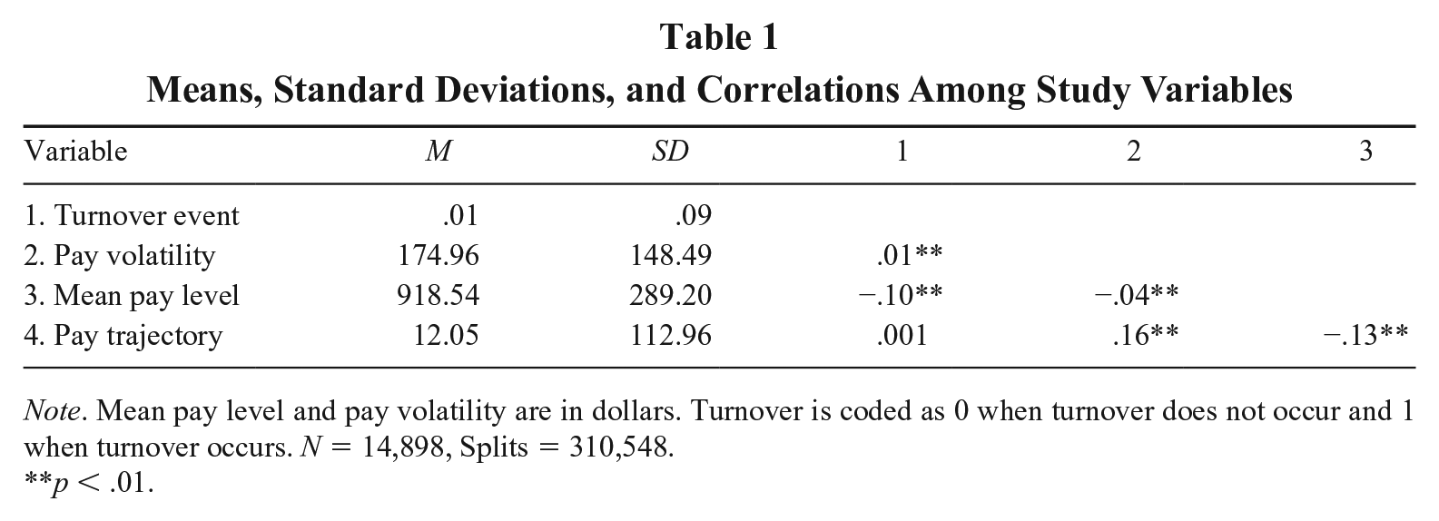
Note. Mean pay level and pay volatility are in dollars. Turnover is coded as 0 when turnover does not occur and 1 when turnover occurs. N = 14,898, Splits = 310,548.

p < .01.

Table 2

Results: Survival Models

Variable	Model 1	Model 2	Model 3	Model 4	Model 5	Model 6
Pay volatility		.0004** (.0001)		.001** (.0001)	.001** (.0001)	−.0004 (.0003)
Mean pay level	−.003** (.0004)	−.003** (.0004)	−.003** (.001)	−.003** (.0001)	−.003** (.0001)	−.003** (.0001)
Pay Volatility × Mean Pay Level						.000001** (.0000003)
Pay trajectory			−.001** (.0002)	−.001** (.0001)	−.001** (.0003)
Pay Volatility × Pay Trajectory					.00000002 (.00001)
Wald test (χ²)	2,323**	2,382**	2,323**	2,376**	2,379**	2,384**
Global χ² (Schoenfeld residuals)	3.38	3.88	3.54	4.32	4.32	3.94
AIC	63,944.50	63,931.92	63,902.72	63,879.11	63,881.11	63,926.39

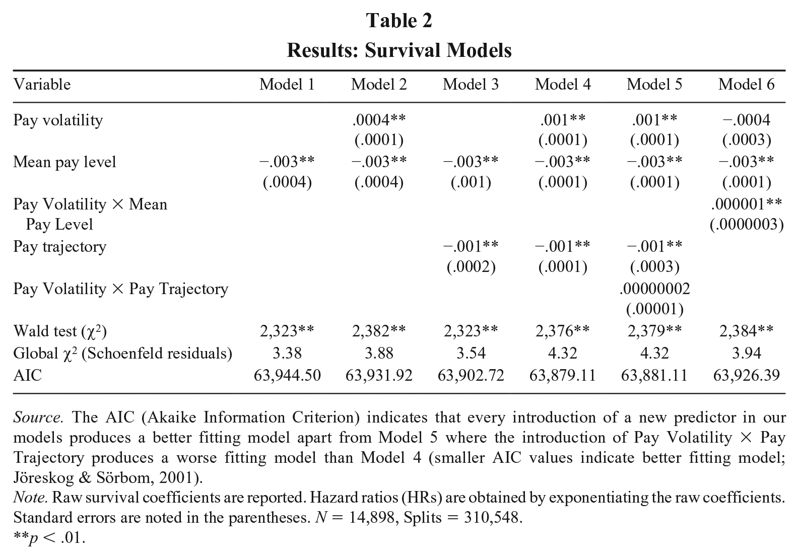
Source. The AIC (Akaike Information Criterion) indicates that every introduction of a new predictor in our models produces a better fitting model apart from Model 5 where the introduction of Pay Volatility × Pay Trajectory produces a worse fitting model than Model 4 (smaller AIC values indicate better fitting model; Jöreskog & Sörbom, 2001).

Note. Raw survival coefficients are reported. Hazard ratios (HRs) are obtained by exponentiating the raw coefficients. Standard errors are noted in the parentheses. N = 14,898, Splits = 310,548.

p < .01.

The first hypothesis suggests that pay volatility is positively related to turnover likelihood. Consistent with Hypothesis 1, Model 2 of Table 2 shows that pay volatility has a significant positive effect on turnover likelihood (HR = 1.0004, p < .001). When pay volatility increases by $1, the likelihood of turnover increases by .04% (holding the effects of other predictors constant). To put this in perspective, a driver whose pay volatility is 1 standard deviation above the mean is 11.88% more likely to turnover compared to a driver whose pay volatility is 1 standard deviation below the mean.

Hypotheses 2 and 3 focus on the role of pay trajectory. Model 3 offers support for the negative relationship between pay trajectory and turnover likelihood (HR = .999, p < .001). Supporting Hypothesis 2, the results indicate that an increase in pay trajectory by one unit will decrease the likelihood of a turnover event by .10%. In other words, a driver whose pay trajectory is 1 standard deviation below the mean is 22.59% more likely to turnover compared to a driver whose pay trajectory is 1 standard deviation above the mean pay trajectory.

Hypothesis 3 suggests that pay trajectory moderates the effect of pay volatility, such that the positive relationship between pay volatility and turnover likelihood is weaker when pay trajectory has an increasing trend. Model 5 of Table 1 indicates that the interaction between pay trajectory and pay volatility was not statistically significant.

Hypothesis 4 proposed that pay level is negatively related to turnover likelihood. The results support this hypothesis (HR = .997, p < .001; see Model 1 of Table 2). Specifically, when pay level increases by $1, the likelihood of turnover decreases by .30%, ceteris paribus. Again, to put this in perspective, a driver whose pay is 1 standard deviation below the mean has a 173.52% higher probability of turnover when compared to a coworker whose pay level is 1 standard deviation above the mean.

The fifth hypothesis stated that mean pay level moderates the relationship between pay volatility and turnover likelihood, such that pay volatility increases turnover likelihood more when mean pay level is low. As Model 6 indicates, the interaction between pay volatility and pay level was statistically significant. To explore this interaction further, an R library protocol called simPH (Gandrud, 2015) was used. SimPH simulates the hazard rates for different values of the two interacting covariates. Thus, we simulated and plotted four hazard rates by combining high (1 SD above mean) and low (1 SD below mean) mean pay levels and high (1 SD above mean) and low (1 SD below mean) pay volatility levels. As Figure 2 illustrates, drivers with high pay volatility and low mean pay levels have the highest turnover likelihood over time, while drivers with low pay volatility and low mean pay level have the second highest turnover likelihood. Drivers with low pay volatility and high mean pay level, as expected, have the lowest likelihood for turnover.

Figure 2

Interaction Plot of Pay Volatility, Pay Level, and Turnover

Robustness Checks

Five different strategies were used to explore the robustness of the results. First, the multicollinearity among predictors was examined. Results of this analysis indicated multicollinearity was not a problem with a variance inflation factor of less than 2.5.

Second, the number of weeks included in the splits was explored. Company leaders suggested a 4-week period, but one additional time frame (8-week split) was also explored. Overall, the results were consistent with our main analysis. The results indicated that all direct effects (i.e., pay volatility, mean pay level, and pay trajectory) on turnover likelihood were statistically significant and in the expected direction. Similarly, the interaction between pay volatility and pay trajectory was nonsignificant. The only difference with the analysis using the 4-week splits is that the results for Model 6 of the 8-week splits analysis indicate that the interaction term between pay volatility and mean pay level is nonsignificant and in the opposite direction. However, when plotting the interaction, the results are consistent with the main analysis (4-week split): Drivers with high pay volatility and low mean pay levels have the highest turnover likelihood over time followed by drivers with low pay volatility and low mean pay level, while the drivers with low pay volatility and high mean pay have the lowest likelihood for turnover. It is important to note that when using the 8-week split, Model 6 was the only model violating the proportionality assumption. So while the interaction was not significant based on this analysis, the nature of the relationship is consistent with our primary analysis. Given that assumptions are violated with the 8-week approach and there was reason to prefer a 4-week interval, we view this analysis as supportive of our findings and approach.

Third, we took a more “traditional” survival analysis approach in order to alleviate any potential concerns, as aptly noted by our reviewers, regarding the choice of the duration of the splits. Specifically, we created a subsample that includes only individuals who were hired during our time frame in order to be able to explore their employment with the specific company in its entirety. In this sample, we had 5,159 truck drivers. All the constructs were dynamic: For each Week t turnover likelihood was explored, every construct was calculated for the entire period of time the drivers were employed by the firm until 1 week before Week t. Recognizing, however, that more recent paychecks are likely to have more weight in the turnover decision, a simple weighting scheme was created. Specifically, if we are looking for the turnover likelihood on Week 9 (thus the constructs capture Weeks 2 to 7), the pay each driver received on Week 7 will have six times more weight than the pay received on Week 2. Again, the results were generally consistent with our main analysis.

The results indicated that all direct effects (i.e., weighted pay volatility, weighted mean pay level, and weighted pay trajectory) on turnover likelihood were statistically significant and in the expected direction. Interestingly, the interaction between the weighted pay volatility and weighted pay trajectory was statistically significant. The plot of the interaction showed that truck drivers who experienced low weighted pay trajectory and low weighted pay volatility had the highest turnover likelihood, followed closely by those who experience low weighted pay trajectory and high weighted pay volatility. Drivers with high weighted pay trajectory and low weighted volatility had the lowest turnover likelihood. The interaction term between weighted pay volatility and weighted mean pay level (Model 6) was statistically significant but in the opposite direction. Again, however, when plotting the interaction, the results remain relatively consistent with our main analysis. Specifically, the highest turnover likelihood is observed for truck drivers with high weighted pay volatility and low weighted mean pay level and the second highest turnover likelihood for truck drivers with low weighted pay volatility and low weighted mean pay level. The only difference with the results of the main analysis is that the lowest turnover likelihood is estimated for truck drivers with high weighted pay volatility and high weighted mean pay level (but the estimated turnover likelihood is very close to those with low weighted pay volatility and high weighted mean pay level). The model exploring the interaction between weighted pay volatility and weighted mean pay level (Model 6) was the only model in this analytical approach that violated the proportionality assumption.

Fourth, acknowledging potential concerns regarding repetitive information of pay for each individual due to the nature of the “rolling” splits we employed in our main analysis, a logistic regression was conducted with no overlapping information. In this analysis, the constructs are calculated over a period of 4 weeks (following the approach used in the main analysis). For the purposes of this analysis, we created a new “matched” subsample. Specifically, in our main sample, the ratio between stayers (individuals who did not leave the company during the time frame we are exploring) and leavers is approximately five to one. Keeping this ratio constant, each leaver was matched with five stayers. The criterion for this “matching” was that the five stayers should have worked for the company for the 4 weeks the constructs were calculated and never left during the time frame of this study. This new sample included 13,880 truck drivers and each truck driver participated only once in the sample. The results indicated that all direct effects (i.e., pay volatility, mean pay level, and pay trajectory) on turnover likelihood were statistically significant and in the expected direction. The interaction between pay volatility and pay trajectory was statistically significant, with higher odds for staying for individuals with high pay volatility and high pay trajectory and lower odds for staying for individuals with low pay volatility and low pay trajectory. For truck drivers with high pay volatility, the odds for staying are lower than those with high pay volatility and relatively unimpacted by pay trajectory. The interaction between mean pay level and pay volatility was not statistically significant.

Finally, following a reviewer’s suggestion, we used an alternative approach to operationalizing pay trajectory. Acknowledging that it is impossible to know the true slope, we created a 95% confidence interval around each trajectory and chose a random slope from that interval. We then reran our analyses using these random slopes. The results were consistent with our main analysis in terms of significance levels and the direction of the relationships.

Discussion

It is easily assumed that organizations benefit from paying only for work needed and completed and that the resulting fluctuations in pay are an unfortunate, but possibly less relevant, side effect. Yet these fluctuations are likely to be problematic for employees as they attempt to meet their financial needs, and these types of pay systems are often in place for the most vulnerable workers in society (Aspen Institute, 2016). In fact, while agency theory asserts that risk is ideally shifted to or at least shared with the agent to ensure aligned interests in firm performance, the agent has the option to walk away from the agreement (Coff, 1997). Thus, organizational leadership must keep this potential for turnover in mind when designing the pay system. The research presented here speaks to this issue by demonstrating that downstream, shifting risk to employee base pay can influence the turnover of employees. And the focus is not on any type of turnover, it is on voluntary turnover that organizations, especially trucking organizations, would prefer to avoid.

The pay fluctuations studied here are at least partially created by the employment policies and practices of the firm. In this research context, an algorithm is the primary determinant of the number of miles a driver can earn pay for each week, which ultimately determines the driver’s paycheck. This algorithm has been designed to optimize routes for the benefit of the company. This explained cause of pay volatility is generally viewed as an acceptable and legitimate approach to distributing pay opportunities, and yet it has dysfunctional consequences for the organization. This algorithmic approach to assigning work has some obvious upsides—there is flexibility to respond to service demand and costs aligned with production (i.e., pay per mile). However, as we demonstrate in this research, there are also downsides to this approach in voluntary turnover. Through our primary analysis as well as several follow-up analyses, we find consistent evidence that pay volatility is positively associated with future turnover likelihood, positive pay trajectories are negatively associated with turnover likelihood, and average pay levels are negatively associated with turnover likelihood.

Theoretical Implications

The present study has numerous implications for theory and future research in compensation and turnover. Foremost, this research addresses pay from a dynamic perspective, which provides a new lens through which to understand base compensation. Compensation research has mainly concerned pay dispersion across employees and employers (Conroy & Gupta, 2019; Downes & Choi, 2014; Gupta, Conroy, & Delery, 2012; Shaw, 2015; Trevor et al., 2012), pay communication/transparency (Bamberger & Belogolovsky, 2017; Fulmer & Chen, 2014), and pay levels and pay changes (Mitra et al., 2016; Shaw, 2014) in recent years; the present research addresses a new approach to studying compensation, which also speaks to these current research streams.

Research on pay dispersion has focused on the bases for pay differences, and scholars generally agree that explained (i.e., productivity-relevant, input-related) dispersion is viewed positively and as fair by employees, while unexplained is more likely to lead to problematic outcomes (Downes & Choi, 2014; Trevor et al., 2012). Our research indicates that this assumption may not apply when we look at pay bases in reference to input-related but not performance-based pay. This suggests that compensation researchers need to dig into this issue and look more closely at the bases of pay. In this study, paychecks are distributed weekly in the focal organization and vary by individual based on units (miles) and, to a lesser extent, driving experience (influencing the pay rate). Most of the fluctuation in miles driven is a function of the loads given to the driver through an automated system. Employees can do little to affect the fluctuations in their pay, yet they are unlikely to view the organization as creating volatility for illegitimate reasons since it is an algorithm based on efficiency that determines miles. Yet we find that volatility created by this legitimate and explained source is associated with turnover. This suggests factors like controllability and predictability may be important to the full picture of pay bases yet have received little research attention.

Our research also suggests that for individual employees, each paycheck is a piece of information that has the potential to be noticed and lead to action in a fairly transparent environment. That is, truck drivers generally have complete knowledge of how paychecks are determined in terms of miles driven and pay per mile. However, there are parts of the pay system that may be less clear; the actual algorithms that determine routes are not always easy to understand. Researchers on pay communication could extend this research by investigating the knowledge and information employees have about the driving factors of pay systems at multiple levels. Does level of understanding of the algorithm change behaviors or strengthen turnover responses?

We integrate the Unfolding Model of Turnover with the literature on pay changes and JND by looking at how pay changes can be shocks. This is somewhat rare because there is a tendency to view wages as “rigid” or “sticky” (i.e., pay does not go down, only up; Favilukis & Lin, 2016), but in many contexts where base pay is variable, changes both upward and downward from week to week are common. Studies of changes related to merit pay cycles are likely to focus on annual fluctuations but only upward changes. For example, Schaubroeck et al. (2008), Folger and Konovsky (1989), and Nyberg (2010) all studied contexts where pay raises were given on an annual basis (interyear volatility). It is both the interval of base pay and the direction of pay changes that has been stagnant from a research perspective. In prior work, shocks would only be expected when annual raises did not meet expectations (Schaubroeck et al., 2008); in our work, we suggest shocks may happen at times outside of the annual raise process. This approach adds nuance to how compensation is viewed in the Unfolding Model of Turnover. Not only are big changes shocks, but week-to-week paychecks can create shocks especially in jobs where volatility is somewhat baked into the pay system (i.e., variable base pay systems).

Our findings militate against rational decision-making approaches to compensation. For example, a rational decision-making perspective on compensation would suggest that pay volatility is irrelevant since the total amount of pay would be equal regardless of fluctuations.² Our findings demonstrate that all is not rational where volatility is concerned as turnover is more likely when pay volatility is high than when it is low. Pushing the rational decision-making logic a bit further and considering the time value of money (i.e., money received sooner is more valuable than money received later; Brigham & Daves, 2019), it could be theorized that large pay amounts early in a timeframe would be more desirable than larger pay amounts at the end of a timeframe, yet our findings demonstrate that positive pay trajectories result in lower likelihood of voluntary turnover. Thus, our findings add to the evidence in compensation that employees react to pay in more psychologically complex ways than basic rationality and that shocks may explain these less than rational reactions.

Our work also contributes to the Unfolding Model of Turnover by exploring a specific type of compensation shock (i.e., pay volatility) along with the context of that shock (i.e., pay level). We find evidence that studying the shifts in pay over a period of 4 weeks predict subsequent turnover. Our time frame of 4 weeks allows us to identify whether there is novelty (i.e., larger shifts are novel) in pay changes as described by Morgeson, Mitchell, and Liu (2015). Future work can build on our treatment of pay volatility as a shock by integrating it with the ideas presented in other work on shocks. For example, Morgeson et al. (2015) also identified criticality (i.e., the importance of the shock) and disruptiveness (i.e., the extent to which the shock disrupts future routines and actions) as features of shocks. Perhaps pay volatility’s effects are dependent on these two factors as well, which could be conceptualized as financial need of the employee and implications of volatility for future pay. This research also demonstrates the importance of internal, organizational shocks on turnover outcomes though we were unable to identify the exact paths to turnover given limitations in our data.

We propose that pay level is more a satisfaction concern, while volatility is the shock-creating mechanism in turnover. This may explain why pay level has a larger impact in our findings than the other pay predictor variables; a level of dissatisfaction with pay level is likely to be relevant in any turnover path since it can be tied to low job satisfaction, it represents a contextual variable that influences the likelihood that a shock will be experienced, and it is a contextual variable that will influence whether the shock leads to actual turnover. Our pay-level findings extend what is known about pay level as a predictor of voluntary turnover (Gerhart & Rynes, 2003; Rubenstein et al., 2018) to demonstrate that this applies even over short periods of time. We also find that the pay level by pay volatility interaction is significant. Higher pay levels appear to buffer volatility’s relationship with future turnover. As one reviewer commented, an alternative logic is that higher pay levels would make an employee more sensitive to volatility if the employee is “living into” their higher pay. Our finding that higher pay levels appear to be more influential in reducing volatility-creating turnover provides further evidence that volatility may be shock-inducing and that pay level is a relevant context for the response to pay volatility. When looking at pay volatility through a JND lens, we propose that the amount of volatility required for a shock is higher when pay level is higher due to the relative nature of JNDs. The importance of these findings is bolstered by the importance of economic factors in turnover. Specifically, economic factors play a large role in turnover, explaining leavers (around 33%) and stayers (around 83%; Donnelly & Quirin, 2006). Our theory is that organizationally driven economic factors can be understood in relation to pay level and pay volatility.

The lack of support in our findings for a pay volatility and pay trajectory interaction points to a potential interesting psychological response to volatility; specifically, the negative bias of individuals (Baumeister et al., 2001) may mean that even when pay is generally headed upward, it does not erase the psychological effects of volatility. On the one hand, perhaps this lack of significance is because when pay volatility is high, the peaks may be followed by troughs even when the overall direction in pay is positive. Thus, while there is a peak in pay and the trajectory is positive, there are still potential “let downs” that outweigh the overall direction, and we know that reductions in pay are generally met with negative responses (Greenberg, 1990; Shaw, 2014). On the other hand, the pay volatility by pay trajectory interaction may also be picking up on ever-increasing pay, a desirable outcome from an employee perspective. The complexity of the psychological processes associated with the volatility and trajectory interaction may have thus prevented the interaction from being significant. Future research exploring the psychological mechanisms over time associated with pay changes could help further explain the relationship between pay trajectory, pay volatility, and turnover.

Practical Implications

The importance of these findings is underscored by their practical relevance. Specifically, an increase of only $1 in pay volatility leads to a change of .04% in the likelihood of turnover. To put this into perspective, a driver whose pay volatility increases by 1 standard deviation ($148.49) over a period of 4 weeks has an almost 6% increased likelihood of turnover. In addition, among our splits we have 137,889 cases where drivers experienced pay volatility that was higher than just 1 standard deviation. More specifically, 12,144 cases indicate that drivers experienced pay volatility that was higher than $500, which translates into at least 20% higher likelihood of turnover. Among those, 734 experienced pay volatility higher than $1,000, which translates in at least 40% higher likelihood of turnover. And turnover is of great concern to companies in the trucking industry (Costello & Karickhoff, 2019).

Thus, this study suggests that pay fluctuations can evoke negative reactions among employees. This is interesting, since the context involves legitimate pay volatility though not performance-based pay volatility. At the organizational level, pay variations across people, when based on legitimate factors, are negatively related to turnover (at least among high and average performers; Shaw & Gupta, 2007). This study demonstrates that pay variations for individuals across time based on legitimate factors increase turnover. Such fluctuations are inevitable in some settings (e.g., commission systems) and likely in others (e.g., varying work schedules).

How can organizations strike a balance between optimizing routes and voluntary turnover? Organizations have the power to design systems that either reduce pay volatility (e.g., set up algorithms with a component to increase the stability of assignments across employees), minimize the downside of pay volatility (e.g., creating a pay floor each week), or reward pay volatility (e.g., compensating volatile earnings with higher rates). When a longer time horizon is considered, pay fluctuations occur in almost all jobs. It is the rare job that pays the same amount over several years. As such, the issue is not one of eliminating pay fluctuations; rather, it is one of minimizing the extent of shocks, especially negative shocks, and their negative effects. Perhaps better design of the algorithm and pay system could be an organizational competitive advantage since it is rare for organizations to take this approach. This is certainly a possibility in the trucking industry where turnover is a substantial concern (Costello & Karickhoff, 2019). We note that such practical concerns indicate a need to study the costs to the company of providing increased stability versus the cost of turnover created by these policies in order to address the possibility that changing the pay approach would be valuable.

Limitations and Boundary Conditions

Several limitations and boundary conditions apply to this study. First, this is a study of employed truck drivers, and generalization beyond this population is open to question. Our study focused on the employment relationship, but modern work in contractor-type relationships (e.g., UBER) also involves significant pay volatility. Thus, it would be valuable for scholars to pursue knowledge of pay volatility’s effects on contractor relationships. Additionally, the measure of pay volatility focused on weekly fluctuations, which may not be applicable to other time intervals. Pay volatility exists in almost all jobs, but the time interval for these variations may be days, weeks, months, or years. Weekly dynamics may not be applicable to other time intervals. This study highlights the fact that it is critical to isolate the key time period for each context that is studied dynamically.

Second, although the concept of perceived shocks was invoked to explain employee reactions, related psychological processes were not measured. Discussions with trucking company management supported the idea that turnover events were often triggered by financial issues, and our finding that pay level moderates the effects further strengthens these arguments. Still, the underlying psychological processes should be measured directly in future research.

Third, and related to the first point, the weekly fluctuations in pay were primarily determined by miles driven and pay rate. Pay variations can be attributable to many legitimate and illegitimate factors such as skill, seniority, and politics (Kepes, Delery, & Gupta, 2009). The effects of fluctuations based on illegitimate factors were not explored in this study. That pay volatility was relatively divorced from performance volatility is both a strength and a boundary condition of the present study. Furthermore, distinguishing pay from the dispatch system is not possible in this study as the dispatch system is the determinant of pay opportunities. We believe pay is the primary driver of our findings because pay provides for many of the needs employees have (Argyle & Furnham, 2013), but there may be an additional nuance to pay volatility. Specifically, it is possible that control over pay volatility is more important than the actual pay volatility. Future studies could help explore this issue either by measuring employee perceptions or using experimental design to distinguish the two factors. Fourth, the sample for this study was necessarily limited to the employees of the organization under study. This meant an overwhelming majority of male drivers in the sample. The results may not apply to more demographically diverse samples.

Countering these limitations and boundary conditions are the numerous strengths of the study. The sample is large. Data from over a 6-month period were used. Measures for the critical pay and turnover variables were obtained from organizational archives and offer relatively “clean” representations of the constructs under study. These strengths go a long way toward mitigating the potential deficiencies of the study.

Conclusion

Temporal fluctuations in pay play a significant role in shaping employee life, and the extent of such fluctuations is often greater for the most vulnerable in the workforce. The results of this research indicate that these fluctuations may not only be problematic for employees but also for organizations as voluntary turnover likelihood increases with greater volatility. This study took steps toward understanding the underlying dynamics of such temporal fluctuations and the implications of these fluctuations, but much work remains.

Footnotes

Acknowledgements

The authors would like to thank Dr. Michael Sturman for providing constructive comments during the development of this manuscript. We would also like to thank Editor David Allen and three anonymous reviewers for their support and insights during the review process.

ORCID iD

Samantha A. Conroy

Notes

References

Allen

D. G.

Bryant

P. C.

Vardaman

J. M.

2010. Retaining talent: Replacing misconceptions with evidence-based strategies. Academy of Management Perspectives, 24: 48-64. doi:10.5465/amp.24.2.48

Allison

P. D.

2009. Fixed effects regression models. Thousand Oaks, CA: Sage. doi:10.4135/9781412993869

Allison

P. D.

2014. Event history and survival analysis: Regression for longitudinal event data, Vol. 46. Thousand Oaks, CA: Sage. doi:10.4135/9781452270029

Argyle

Furnham

2013. The psychology of money. London: Routledge. doi:10.4324/9781315812496

Aspen Institute. 2016. Income volatility: A primer. Retrieved August 8, 2019, from The Aspen Institute: https://assets.aspeninstitute.org/content/uploads/files/content/docs/pubs/EPIC+Volatility+Primer+(May).pdf

Bamberger

Belogolovsky

2017. The dark side of transparency: How and when pay administration practices affect employee helping. Journal of Applied Psychology, 102: 658-671. doi:10.1037/apl0000184

Baumeister

R. F.

Bratslavsky

Finkenauer

Vohs

K. D.

2001. Bad is stronger than good. Review of General Psychology, 5: 323-370. doi:10.1037/1089-2680.5.4.323

Box-Steffensmeier

J. M.

Jones

B. S.

2004. Event history modeling: A guide for social scientists. New York, NY: Cambridge University Press. doi:10.1017/cbo9780511790874

Breslow

N. E.

1972. Discussion of the paper by D.R. Cox. Journal of the Royal Statistical Society, 34: 216-217. doi:10.1080/10485250500491661

10.

Brigham

E. F.

Daves

P. R.

2019. Intermediate financial management. Australia: Cengage.

11.

Chen

Ployhart

R. E.

Thomas

H. C.

Anderson

Bliese

P. D.

2011. The power of momentum: A new model of dynamic relationships between job satisfaction change and turnover intentions. Academy of Management Journal, 54: 159-181. doi:10.5465/AMJ.2011.59215089

12.

Coff

R. W.

1997. Human assets and management dilemmas: Coping with hazards on the road to resource-based theory. Academy of Management Review, 22: 374-402. doi:10.2307/259327

13.

Conroy

S. A.

Gupta

2019. Disentangling horizontal pay dispersion: Experimental evidence. Journal of Organizational Behavior, 40: 248-263. doi:10.1002/job.2323

14.

Costello

Karickhoff

2019. Truck driver shortage analysis. Retrieved from https://www.trucking.org/sites/default/files/2020-01/ATAs%20Driver%20Shortage%20Report%202019%20with%20cover.pdf

15.

Costello

Suarez

2015. Truck driver shortage analysis. Retrieved from http://www.trucking.org/ATA%20Docs/News%20and%20Information/Reports%20Trends%20and%20Statistics/10%206%2015%20ATAs%20Driver%20Shortage%20Report%202015.pdf

16.

Cox

D. R.

1972. Regression models and life tables. Journal of the Royal Statistical Society, B34: 187-220. doi:10.1111/j.2517-6161.1972.tb00899.x

17.

Davis

P. R.

Trevor

C. O.

Feng

2015. Creating a more quit-friendly national workforce? Individual layoff history and voluntary turnover. Journal of Applied Psychology, 100: 1434-1455. doi:10.1037/apl0000012

18.

Donnelly

D. P.

Quirin

J. J.

2006. An extension of Lee and Mitchell’s unfolding model of voluntary turnover. Journal of Organizational Behavior, 27: 59-77. doi:10.1002/job.367

19.

Downes

P. E.

Choi

2014. Employee reactions to pay dispersion: A typology of existing research. Human Resource Management Review, 24: 53-66. doi:10.1016/j.hrmr.2013.08.009

20.

Efron

1977. The efficiency of Cox’s likelihood function for censored data. Journal of American Statistical Association, 72: 557-565. doi:10.1080/01621459.1977.10480613

21.

Favilukis

Lin

2016. Does wage rigidity make firms riskier? Evidence from long-horizon return predictability. Journal of Monetary Economics, 78: 80-95. doi:10.1016/j.jmoneco.2016.01.003

22.

Folger

Konovsky

M. A.

1989. Effects of procedural and distributive justice on reactions to pay raise decisions. Academy of Management Journal, 32(1): 115-130. doi:10.2307/256422

23.

Fox

2002. Cox proportional-hazards regression for survival data. In Fox

(Ed.), An R and S-PLUS companion to applied regression: 1-18. Thousand Oaks, CA: Sage. doi:10.1.1.110.2264

24.

Fulmer

I. S.

Chen

2014. How communication affects employee knowledge of and reactions to compensation systems. In Miller

Gordon

(Eds.), Meeting the challenge of human resource management: A communication perspective: 167-178. New York, NY: Routledge/Taylor & Francis.

25.

Gandrud

2015. simPH: An R package for illustrating estimates from Cox proportional hazard models including for interactive and nonlinear effects. Journal of Statistical Software, 65: 1-20. doi:10.2139/ssrn.2318977

26.

Gerhart

Rynes

2003. Compensation: Theory, evidence, and strategic implications. Thousand Oaks, CA: Sage. doi:10.4135/9781452229256

27.

Greenberg

1990. Employee theft as a reaction to underpayment inequity: The hidden cost of pay cuts. Journal of Applied Psychology, 75: 561-568. doi:10.1037/0021-9010.75.5.561

28.

Gupta

Conroy

S. A.

Delery

J. E.

2012. The many faces of pay variation. Human Resource Management Review, 22: 100-115. doi:10.1016/j.hrmr.2011.12.001

29.

Gupta

Shaw

J. D.

2014. Employee compensation: The neglected area of HRM research. Human Resource Management Review, 24: 1-4. doi:10.1016/j.hrmr.2013.08.007

30.

Hausknecht

J. P.

Sturman

M. C.

Roberson

Q. M.

2011. Justice as a dynamic construct: Effects of individual trajectories on distal work outcomes. Journal of Applied Psychology, 96: 872-880. doi:10.1037/ a0022991

31.

Holtom

B. C.

Inderrieden

E. J.

2006. Integrating the unfolding model and job embeddedness model to better understand voluntary turnover. Journal of Managerial Issues, 18: 435-452.

32.

Holtom

B. C.

Mitchell

T. R.

Lee

T. W.

Inderrieden

E. J.

2005. Shocks as causes of turnover: What they are and how organizations can manage them. Human Resource Management, 44: 337-352. doi:10.1002/hrm.20074

33.

Hom

P. W.

Allen

D. G.

Griffeth

R. W.

2020. Employee retention and turnover: Why employees stay or leave. New York: Routledge. doi:10.4324/9781315145587

34.

Jöreskog

K. G.

Sörbom

2001. LISREL 8.5: Structural equation modeling with the SIMPLIES command language. Chicago: Scientific Software International.

35.

Judge

T. A.

Piccolo

R. F.

Podsakoff

N. P.

Shaw

J. C.

Rich

B. L.

2010. The relationship between pay and job satisfaction: A meta-analysis of the literature. Journal of Vocational Behavior, 77: 157-167. doi:10.1016/j.jvb.2010.04.002

36.

Kammeyer-Mueller

J. D.

Wanberg

C. R.

Glomb

T. M.

Ahlburg

2005. The role of temporal shifts in turnover processes: It’s about time. Journal of Applied Psychology, 90: 644-658. doi:10.1037/0021-9010.90.4.644

37.

Kepes

Delery

Gupta

2009. Contingencies in the effects of pay range on organizational effectiveness. Personnel Psychology, 62(3): 497-531. doi:10.1111/j.1744-6570.2009.01146.x

38.

Lee

T. W.

Hom

P. W.

Eberly

M. B.

Mitchell

T. R.

2017. On the next decade of research in voluntary employee turnover. Academy of Management Perspectives, 31: 201-221. doi:10.5465/amp.2016.0123

39.

Lee

T. W.

Mitchell

T. R.

1994. An alternative approach: The unfolding model of voluntary employee turnover. Academy of Management Review, 19(1): 51-89. doi:10.2307/258835

40.

March

J. G.

Simon

H. A.

1958. Organizations. New York: John Wiley & Sons, Inc. doi:10.4236/ojmh.2012.21002

41.

Mas

Pallais

2017. Valuing alternative work arrangements. American Economic Review, 107: 3722-3759. doi:10.1257/aer.20161500

42.

Mickel

A. E.

Barron

L. A.

2008. Getting “more bang for the buck” symbolic value of monetary rewards in organizations. Journal of Management Inquiry, 17: 329-338. doi:10.1177/1056492606295502

43.

Mitchell

D. S.

2017. Stable and predictable scheduling as antidote to income volatility. Retrieved from http://www.aspenepic.org/wp-content/uploads/2017/04/Issue-Brief-3-Predictable-Schedling.pdf

44.

Mitchell

T. R.

Mickel

A. E.

1999. The meaning of money: An individual-difference perspective. Academy of Management Review, 24: 568-578. doi:10.5465/amr.1999.2202138

45.

Mitra

Gupta

Jenkins

G. D.

Jr.

1997. A drop in the bucket: When is a pay raise a pay raise? Journal of Organizational Behavior, 18: 117-137. doi:10.1002/(SICI)1099-1379(199703)18:23.0.CO;2-1

46.

Mitra

Tenhiälä

Shaw

J. D.

2016. Smallest meaningful pay increases: Field test, constructive replication, and extension. Human Resource Management, 55: 69-81. doi:10.1002/hrm.21712

47.

Morgeson

F. P.

Mitchell

T. R.

Liu

2015. Event system theory: An event-oriented approach to the organizational sciences. Academy of Management Review, 40: 515-537. doi:10.5465/amr.2012.0099

48.

Morita

J. G.

Lee

T. W.

Mowday

R. T.

1993. The regression-analog to survival analysis: A selected application to turnover research. Academy of Management Journal, 36: 1430-1464. doi:10.5465/256818

49.

Nyambegera

S. M.

Sparrow

Daniels

2000. The impact of cultural value orientations on individual HRM preferences in developing countries: Lessons from Kenyan organizations. International Journal of Human Resource Management, 11: 639-663. doi:10.1080/09585190050075042

50.

Nyberg

2010. Retaining your high performers: Moderators of the performance-job satisfaction-voluntary turnover relationship. Journal of Applied Psychology, 95: 440-453. doi:10.1037/a0018869

51.

Page

1998. Survival analysis in psychology: Effects of censoring and proportionality. Doctoral dissertation, 98-105 Arizona State University. doi:10.1213/ANE.0000000000003653

52.

Porter

L. W.

Steers

R. M.

1973. Organizational, work, and personal factors in employee turnover and absenteeism. Psychological Bulletin, 80: 151-176. doi:10.1037/h0034829

53.

Puranam

Singh

Zollo

2006. Organizing for innovation: Managing the coordination-autonomy dilemma in technology acquisitions. Academy of Management Journal, 49: 263-280. doi:10.5465/amj.2006.20786062

54.

Rogosa

D. R.

Willett

J. B.

1985. Understanding correlates of change by modeling individual differences in growth. Psychometrika, 50: 203-228. doi:10.1007/BF02294247

55.

Rubenstein

A. L.

Eberly

M. B.

Lee

T. W.

Mitchell

T. R.

2018. Surveying the forest: A meta-analysis, moderator investigation, and future-oriented discussion of the antecedents of voluntary employee turnover. Personnel Psychology, 71: 23-65. doi:10.1111/peps.12226

56.

Rynes

S. L.

Gerhart

Minette

K. A.

2004. The importance of pay in employee motivation: Discrepancies between what people say and what they do. Human Resource Management, 43: 381-394. doi:10.1002/hrm.20031

57.

Salamin

Hom

P. W.

2005. In search of the elusive U-shaped performance-turnover relationship: Are high performing Swiss bankers more liable to quit? Journal of Applied Psychology, 90: 1204-1216. doi:10.1037/0021-9010.90.6.1204

58.

Schaubroeck

Shaw

J. D.

Duffy

M. K.

Mitra

2008. An under-met and over-met expectations model of employee reactions to merit raises. Journal of Applied Psychology, 93: 424-434. doi:10.1037/0021-9010.93.2.424

59.

Schemper

1992. Cox analysis of survival data with non-proportional hazard functions. Statistician, 41: 455-465. doi:10.2307/2349009

60.

Shaw

J. D.

2014. Pay levels and pay changes. In Handbook of industrial, work, and organizational psychology. Thousand Oaks, CA: Sage. doi:10.4135/9781473914957

61.

Shaw

J. D.

2015. Pay dispersion, sorting, and organizational performance. Academy of Management Discoveries, 1: 165-179. doi:10.5465/amd.2014.0045

62.

Shaw

J. D.

Delery

J. E.

Jenkins

G. D.

Jr. Gupta

1998. An organization-level analysis of voluntary and involuntary turnover. Academy of Management Journal, 41: 511-525. doi:10.5465/256939

63.

Shaw

J. D.

Gupta

2007. Pay system characteristics and quit patterns of good, average, and poor performers. Personnel Psychology, 60: 903-928. doi:10.1111/j.1744-6570.2007.00095.x

64.

Sheridan

J. E.

1992. Organizational culture and employee retention. Academy of Management Journal, 35: 1036-1056. doi:10.2307/256539

65.

Singer

J. D.

Willet

J. B.

2003. A framework for investigating change over time. In Applied longitudinal data analysis: Modeling change and event occurrence: 3-15. doi:10.1093/acprof:oso/9780195152968.003.0001 New York: Oxford University Press.

66.

Sturman

2007. The past, present, and future of dynamic performance research. Research in Personnel and Human Resources Management, 26: 49-110. doi:10.1016/s0742-7301(07)26002-5

67.

Sturman

M. C.

Trevor

C. O.

2001. The implications of linking the dynamic performance and turnover literatures. Journal of Applied Psychology, 86: 684-696. doi:10.1037/0021-9010.86.4.684

68.

Suarez

F. F.

Utterback

J. M.

1995. Dominant designs and the survival of firms. Strategic Management Journal, 16: 415-430. doi:10.1002/smj.4250160602

69.

Therneau

Crowson

Atkinson

2017. Using time dependent covariates and time dependent coefficients in the Cox model. R package Survival Vignettes version 2.41 https://cran.r-project.org/web/packages/survival/vignettes/. https://cran.r-project.org/web/packages/survival/vignettes/timedep.pdf

70.

Trevor

C. O.

Reilly

Gerhart

2012. Reconsidering pay dispersion’s effect on the performance of interdependent work: Reconciling sorting and pay inequality. Academy of Management Journal, 55: 585-610. doi:10.5465/amj.2006.0127

71.

Weller

Holtom

B. C.

Matiaske

Mellewigt

2009. Level and time effects of recruitment sources on early voluntary turnover. Journal of Applied Psychology, 94: 1146-1162. doi:10.1037/a0015924

72.

Whitaker

2010. Driver turnover costs, causes and solutions. Avatar Management Services Inc. White Paper. Retrieved from https://docplayer.net/21311496-Driver-turnover-costs-causes-and-solutions.html

73.

Williams

M. L.

McDaniel

M. A.

Nguyen

N. T.

2006. A meta-analysis of the antecedents and consequences of pay level satisfaction. Journal of Applied Psychology, 91: 392-413. doi:10.1037/0021-9010.91.2.392

74.

Young

G. J.

Charns

M. P.

Shortell

S. M.

2001. Top manager and network effects on the adoption of innovative management practices: A study of TQM in a public hospital system. Strategic Management Journal, 22: 935-951. doi:10.1002/smj.194