A Comment on Tobias Kronenberg’s “Construction of Regional Input-Output Tables Using Nonsurvey Methods: The Role of Cross-Hauling”

Abstract

This article examines the effectiveness of a new non-survey regionalization method: Kronenberg’s Cross-Hauling Adjusted Regionalization Method (CHARM). This aims to take into account the fact that regions typically both import and export most commodities. Data for Uusimaa, Finland’s largest region, are employed to carry out a detailed empirical test of CHARM. This test gives very encouraging results. CHARM is suitable for studying environmental questions, but it can only be applied in situations where foreign imports have been included in the national input–output table. Where the focus is on regional output and employment, location quotients (LQs) can be used for purposes of regionalization. On both theoretical and empirical grounds, the FLQ appears to be the most suitable LQ currently available. It should be applied to national input–output tables that exclude foreign imports. Both types of table are available at the national level for all European Union members as well as for some other countries.

Keywords

regional input–output tables cross-hauling location quotients CHARM FLQ

Introduction

Regional scientists have tried for several decades to develop a satisfactory way of “regionalizing” national input−output tables, so that adequate regional tables can be produced at an acceptable cost, but the phenomenon of cross-hauling has bedeviled their efforts. Cross-hauling occurs when a sector simultaneously imports and exports the same commodity. This is a chronic problem in small regions that do not represent a functional economic area (Robison and Miller 1988), but it is also problematic in larger regions (Kronenberg 2009). It is apt to be more serious in densely populated and highly urbanized countries, especially those where commuting across regional boundaries is important (Boomsma and Oosterhaven 1992, 272−73). Kronenberg highlights the heterogeneity of products as the main cause of cross-hauling; he illustrates this point by referring to the fact that interregional trade in automobiles occurs in Germany, with BMWs being transported from Bavaria to Lower Saxony and Volkswagens being sent in the opposite direction, despite the fact that, in principle, each region could be self-sufficient in its own marque (Kronenberg 2009, 49). Conventional approaches to regionalization fail to account for cross-hauling and this shortcoming results in an underestimation of interregional trade and hence an overstatement of regional multipliers. Kronenberg proposes a new way of dealing with this problem, which he calls the Cross-Hauling Adjusted Regionalization Method (CHARM). Before examining his proposal, however, some pertinent issues need to be considered concerning the nature of published national input−output tables and the different ways in which they can be adapted to correspond to the structure of regional economies.

Format of Input−Output Tables

Published input−output tables can take several alternative forms, ranging from type A to type E.¹ This nomenclature follows Kronenberg (2011) and the United Nations (1973). At the outset, let us examine the traditional type B table. An illustration is given by the survey-based tables for 1995 constructed by Statistics Finland (2000) for the whole country as well as for each of its twenty regions. These tables are based on an identical set of thirty-seven sectors, which is very convenient as it avoids awkward problems that arise when aggregation of national sectors is required.

Table 1 shows extracts from the tables for Finland and Etelä–Pohjanmaa (E-P), a region that generated 2.9 percent of Finnish output in 1995.² For simplicity, only five supplying sectors and one purchasing sector are shown. The table reveals that intermediate inputs sourced from within the E-P region accounted for 35.5 percent of the gross output of meat and fish, whereas other Finnish regions accounted for 51.4 percent. However, taken together, intermediate inputs emanating from within Finland accounted for 86.9 percent of the gross output of meat and fish in this region, which does not differ greatly from the figure of 83.7 percent for the national industry. It may be noted, finally, that the proportion of intermediate inputs obtained from abroad is very similar for the national and regional industries, as is the pattern of primary inputs.

Table 1.

Input Coefficients in Finland in 1995.

	Etelä-Pohjanmaa	Finland
	Meat and Fish	Meat and Fish
01 Agriculture	0.2404	0.3594
06 Meat and fish	0.0350	0.2998
26 Hotels and restaurants	0.0007	0.0018
27 Transport	0.0315	0.0324
33 Renting and business activities	0.0115	0.0300
Total use of domestic products at basic prices	0.3547	0.8365
Total use of imported products	0.5139	0.0000
Foreign imports	0.0536	0.0576
Value-added tax plus other taxes on products	0.0017	0.0025
Subsidies on products	−0.1372	−0.1250
Total intermediate consumption at purchasers' prices	0.7866	0.7716
Compensation of employees	0.1385	0.1485
Other taxes on production	0.0001	0.0007
Subsidies on production	−0.0014	−0.0043
Other value added	0.0761	0.0835
Value added at basic prices	0.2134	0.2284
Output at basic prices	1.0000	1.0000

Note. Figures in bold are subtotals, e.g. 0.7866 + 0.2134 = 1.0000.

The interpretation of the coefficients now needs to be considered. The regional input coefficients, the r_ij , measure the number of units of regional input i needed to produce one unit of gross output of regional industry j, for example, r _1,6 = 0.2404. These coefficients encompass intermediate inputs produced in the region under consideration but exclude inputs from other Finnish regions or from abroad. By contrast, the national input coefficients, the a_ij , measure the number of units of national input i needed to produce one unit of gross output of national industry j, for example, a ₆,₆ = 0.2998. These coefficients encompass intermediate inputs originating from within Finland but exclude inputs from other countries. It should be noted that the a_ij are sometimes erroneously referred to as national technical coefficients, a problem that is highlighted by Hewings and Jensen (1986).

Type A tables differ from type B tables in terms of the way in which imports are treated and this has important implications for the meaning of the input coefficients. In a type A national table, foreign imports are allocated indirectly to the industries that use these imports as intermediate inputs. For example, foreign steel used by the automobile industry would be included as an intermediate input for this industry; it would thus appear in the relevant row for steel and column for automobiles in the interindustry matrix.

In a type A table, the input coefficients, the a_ij *, measure the number of units of input i needed to produce one unit of gross output of national industry j. These coefficients encompass intermediate inputs originating not just from within Finland but also from other countries. The a_ij * are true national technical coefficients because they reflect the underlying technology and are not affected by the pattern of trade. It is not possible to derive estimates of the a_ij * from Table 1 because foreign imports are not disaggregated by sector.

In addition to tables of types A and B, members of the European Union (EU) produce symmetric national tables that are a variant of type A; these are referred to here as type E tables (E stands for Eurostat, the statistical office in the EU). This is the tabular format discussed in Kronenberg (2009). The German tables he discusses, which he refers to as ESA 95 tables, are compiled in accordance with the rules of the European System of Accounts (ESA). ESA 95 is the standard for all EU countries. However, since the ESA 95 rules also apply to the other types of table, the tables Kronenberg discusses will be referred to here as type E tables rather than as ESA 95 tables. Type E tables can easily be derived from those of type A; all that is required is to transpose the column vector of total imports by commodity to produce a row vector of total imports (from other regions and from abroad) by industry. Furthermore, by summing output and imports, one can estimate total supply by industry and hence compute supply multipliers. These should not be confused with the type I output multipliers that are associated with type B tables.

Location Quotients

Location quotients (LQs) are a popular way of regionalizing national input−output tables, especially in the initial stages. For this purpose, the following alternative LQs are often used:

{S L Q}_{i} \equiv \frac{{R E}_{i} / T R E}{{N E}_{i} / T N E} \equiv \frac{{R E}_{i}}{{N E}_{i}} \times \frac{T N E}{T R E},

{C I L Q}_{i j} \equiv \frac{{S L Q}_{i}}{{S L Q}_{j}} \equiv \frac{{R E}_{i} {/ N E}_{i}}{{R E}_{j} {/ N E}_{j}},

where SLQ _i is the simple LQ, CILQ _ij is the cross-industry LQ, RE _i is regional employment (or output) in supplying sector i, and NE _i is the corresponding national figure. RE _j and NE _j are defined analogously for purchasing sector j. TRE and TNE are the respective regional and national totals.

So long as no aggregation of national sectors is required, the following simple formula can be used to convert national into regional input coefficients:

r_{i j} = β_{i j} \times a_{i j},

where r_ij is the regional input coefficient, β _ij is an adjustment coefficient and a_ij is the national input coefficient, derived from a type B table. r_ij measures the amount of regional input i needed to produce one unit of regional gross output j; it thus excludes any supplies of i “imported” from other regions or obtained from abroad. a_ij likewise excludes any supplies of i obtained from abroad. The role of β _ij is to take account of a region’s purchases of input i from other regions.

If we replace β _ij in equation (3) with SLQ _i or CILQ _ij , we can obtain estimates of the r_ij . Thus, for instance:

{\hat{r}}_{i j} = {S L Q}_{i} \times a_{i j} .

Note: No adjustment is made to the national coefficient where SLQ _i ≥ 1 or CILQ _ij ≥ 1. We now need to consider how these conventional LQs deal with cross-hauling. In fact, the SLQ rules out the possibility of cross-hauling a priori. It presupposes that a region will import from other regions, yet not export to them, if SLQ _i < 1 but do the opposite if SLQ _i ≥ 1. The CILQ does not preclude cross-hauling, as some cells in a given row of the adjustment matrix can have CILQ _ij < 1, while others can have CILQ _ij ≥ 1. Hence imports and exports of commodity i can occur simultaneously.³ The problem is that the CILQ does not make adequate allowance for cross-hauling, so that it still tends to underestimate imports from other regions and hence to overstate regional multipliers.

Flegg, Webber, and Elliott (1995) attempted to overcome this underestimation of interregional trade via their FLQ formula. In its refined form (Flegg and Webber 1997), the FLQ is defined as:

{F L Q}_{i j} \equiv {C I L Q}_{i j} \times λ^{*} f o r i \neq j,

{F L Q}_{i j} \equiv {S L Q}_{i} \times λ^{*} f o r i = j,

where:

λ^{*} = {[{l o g}_{2} (1 + T R E / T N E)]}^{δ} .

0 ≤ δ < 1; as δ increases, so too does the allowance for interregional imports. δ = 0 represents a special case where FLQ _ij = CILQ _ij . As with other LQ-based formulae, the FLQ is constrained to unity.

By taking explicit account of the relative size of a region, the FLQ should help to address the problem of cross-hauling, which is more likely to be prevalent in smaller regions than in larger ones. Smaller regions are apt to be more open to interregional trade.

Use of LQs

Kronenberg argues (2009, p. 48) that “LQ methods should not be applied to ESA 95 tables.” We presume that he is referring here to tables of types A and E; if so, we are in full agreement. Nevertheless, his rationale is worth examining. Kronenberg cites the use of an equation like 4, where SLQ _i is employed to scale the a_ij rather than the a_ij *. The SLQ would not, therefore, capture any differences between regional and national trading patterns with respect to foreign imports. This criticism echoes one by Hewings and Jensen (1986), who are quoted by Kronenberg (2009, p. 47) thus: “The only manner in which the logic of the CB and quotient techniques can be validated is to apply the techniques to the [national technical coefficients], and this would require further adjustment of the national input-output table” (p. 310). Note: CB denotes commodity balance, a concept to be discussed later.

Our understanding of Hewings and Jensen’s argument is that, if LQs are used, they should be applied to national input coefficients that incorporate inputs from abroad, that is, to the a_ij * rather than to the a_ij . Indeed, in the well-known GRIT (Generation of Regional Input−Output Tables) procedure, phase I involves adding foreign inputs to domestic inputs to produce an estimated national technical coefficients matrix. This phase is followed by a second one, in which LQs are employed to adjust for regional imports (West 1990, 107−8). Hewings and Jensen’s argument appears to suggest, therefore, that LQ methods should be applied to tables with indirectly allocated imports (types A and E), whereas Kronenberg contends that they should not. Let us now explore this argument.

At the outset, some definitions are required. Let:

a_{i j} = t_{i j}^{n} \times a_{i j}^{*} .

Likewise, for a region,

r_{i j} = t_{i j}^{r} \times r_{i j}^{*},

where t_ij ⁿ and t_ij ^r are the respective national and regional trading coefficients, 0 ≤ t_ij ⁿ , t_ij ^r ≤ 1, while a_ij * and r_ij * are the corresponding technical coefficients. In particular, r_ij * measures the number of units of input i, regardless of source, needed to produce one unit of regional gross output j. If we assume that r_ij * = a_ij *, then

r_{i j} = t_{i j}^{r} \times a_{i j}^{*} .

Furthermore,

r_{i j} = (t_{i j}^{r} / t_{i j}^{n}) \times a_{i j} .

Equations (10) and (11) offer alternative routes to estimating the r_ij , so which one should the analyst pursue? In earlier times, the paucity of relevant data meant that using equation (10) would have involved the awkward task of reallocating intermediate imports to individual cells of the transactions matrix. Nowadays, however, in the case of the EU and some other countries (e.g., Australia, Japan, and Mexico), the necessary data are readily available, so the regional analyst faces a genuine choice.

There is, in fact, a compelling reason why it is inadvisable to apply LQs to the national technical coefficients. To illustrate this point, consider the case of the manufacture of basic metals and fabricated metal products (sector 11 in the regional tables discussed later). A region that did not produce such items would have SLQ₁₁ = CILQ_{11, j} = 0. Using equation (10), we would set all input coefficients in row 11 of the type A regional table equal to zero, which would be tantamount to saying that industries in that region made no use whatsoever of such inputs. Equation (11), on the other hand, would yield much more sensible results. As before, we would set all input coefficients in row 11 of the type B regional table equal to zero but the required imports would be included under foreign and domestic imports.

Furthermore, Flegg and Webber (1997, 801) argue that the a_ij * “reflect commodities produced by both domestic and foreign workers and they thus provide a questionable theoretical basis for the application of LQs derived from domestic employment.” They go on to suggest (ibid.) that LQs should be regarded not as trading coefficients but instead as adjustment formulae that:

attempt to capture differences in the regional and national ability to fulfil the needs of purchasing sectors. Such differences are likely to be reflected in the ratio RE_i/NE_i and hence in the SLQ and CILQ. This ratio is also likely to reflect differences in regional and national propensities to import foreign goods; m_ij ^r > m_ij ⁿ would produce a lower RE_i/NE_i and vice versa. On this interpretation, greater import penetration − whether from abroad or from other regions—would be reflected in lower regional employment and hence in smaller LQs.

In view of the above arguments, we would say that Kronenberg is right to contend that LQ methods should not be applied to tables with indirectly allocated imports (types A and E). We now need to consider exactly what is involved in using LQs to estimate the value of the ratio (t_ij ^r /t_ij ⁿ ) in equation (11). First, let us decompose t_ij ^r , which represents the proportion of regional output supplied by regional producers, as follows:

t_{i j}^{r} = (1 - p_{j}^{r a}) - p_{j}^{r s},

where p_j ^ra and p_j ^rs are the regional propensities to import from abroad and from other regions, respectively, in a particular industry j. These propensities are assumed, for simplicity, to be invariant across supplying sectors. Dividing through by t_ij ⁿ yields the expression:

\frac{t_{i j}^{r}}{t_{i j}^{n}} = [\frac{1 - p_{j}^{r a}}{1 - p_{j}^{n a}} - \frac{p_{j}^{r s}}{1 - p_{j}^{n a}}],

so that, from equation (11), we obtain:

r_{i j} = [\frac{1 - p_{j}^{r a}}{1 - p_{j}^{n a}} - \frac{p_{j}^{r s}}{1 - p_{j}^{n a}}] \times a_{i j} .

Furthermore, if we assume that p_j ^ra = p_j ^na , we get:

r_{i j} = [1 - \frac{p_{j}^{r s}}{1 - p_{j}^{n a}}] \times a_{i j} .

The bracketed terms in equations (14) and (15) measure the tendency for a region to source its inputs from within its borders and it is this tendency that LQs attempt to proxy. The FLQ should be well placed to accomplish this task, since it takes into account the relative size of the supplying and purchasing sectors, along with the relative size of the region.

To clarify the meaning of equation (14), we can make use of the data shown in Table 1. The values of the variables can be derived as follows:

Foreign import propensity for Finland: 0.0576/0.8941 = 0.0644, so $1 - p_{j}^{n a} = 0.9356$

Foreign import propensity for E-P: 0.0536/0.9222 = 0.0581, so $1 - p_{j}^{r a}$ = 0.9419

E-P’s propensity to import from other regions: 0.5139/0.9222 = 0.5573

Hence $[\frac{0.9419}{0.9356} - \frac{0.5573}{0.9356}] = 1.0067 - 0.5957 = 0.411, s o t h a t {\hat{r}}_{i j} = 0.411 \times a_{i j} .$

The scalar 0.411 gives us a rough estimate of what is needed for a “typical” supplying sector. If we assume that p_j ^ra = p_j ^na , equation (15) yields a scalar of 0.404, which shows that the divergence between the national and regional propensities to import from abroad has a negligible impact in this instance.

It is worth noting that the ratio (t_ij ^r /t_ij ⁿ ) in equation (11) can exceed unity, which means that it can encompass cases where r_ij > a_ij . Such cases are catered for by the augmented FLQ (AFLQ), which includes a regional specialization term. However, the empirical evidence suggests that this more complex adjustment formula does not yield significantly better results (Flegg and Webber 2000; Bonfiglio and Chelli 2008; Flegg and Tohmo 2011).

Performance of the FLQ

Kronenberg (2009) remarks that the FLQ approach “has met with mixed success” (p. 49). However, we would say that this evaluation fails to give due weight to the considerable body of published evidence that demonstrates the clear superiority of the FLQ over the conventional LQs, although it is true that some of this evidence was not available at the time Kronenberg was writing. This evidence includes studies using survey-based data for Peterborough (Flegg, Webber, and Elliott 1995), Scotland (Flegg and Webber 2000), one Finnish region (Tohmo 2004), all Finnish regions (Flegg and Tohmo 2011), along with the Monte Carlo study by Bonfiglio and Chelli (2008), who examined 400,000 sectoral output multipliers. On the other hand, Riddington, Gibson, and Anderson (2006) found the FLQ to be unhelpful, albeit on the basis of findings pertaining to a single sector in one Scottish region (Flegg and Tohmo 2011).

Now let us consider some key findings of Flegg and Tohmo (2011), who examined data for all twenty Finnish regions in 1995, using survey-based type B tables containing thirty-seven sectors. They used the following criteria to assess the relative performance of the FLQ and the conventional LQs in estimating type I sectoral output multipliers:

μ_{1} = (100 / n) \sum_{j} ({\hat{m}}_{j} - m_{j}) / m_{j},

μ_{2} * = 100 (\bar{\hat{m}} - \bar{m}) / (\bar{m} - 1),

μ_{3} = 100 \sum_{j} q_{j} ({\hat{m}}_{j} - m_{j}) / m_{j},

μ_{4} = 100_{} \sqrt{\frac{\sum_{j} ({\hat{m}}_{j} - m_{j})^{2}}{\sum_{j} m_{j}^{2}}},

μ_{5} = (1 / n) \sum_{j} | {\hat{m}}_{j} - m_{j} | / m_{j},

S D = {[(1 / n) \sum_{j} {\{(|{\hat{m}}_{j} - m_{j}| / m_{j}) - μ_{5}\}}^{2}]}^{0.5},

where

{\hat{m}}_{j}

is the estimated type I output multiplier for sector j (column sum of the LQ-based Leontief inverse matrix) in a given region, m_j is the corresponding survey-based multiplier, q_j is the proportion of regional output produced in sector j and n = 37 is the number of sectors.

Table 2 reveals that the FLQ—irrespective of which statistic is used—yields far more accurate results than the SLQ and CILQ. The most likely explanation of this outcome is that the SLQ and CILQ make inadequate downward adjustments to the national input coefficients, to allow for imports from other regions, and hence greatly understate regional propensities to import. The strong upward bias in input coefficients and hence multipliers is also manifested by the similarity in the mean values of μ₁ and μ₅ for the SLQ and likewise for the CILQ.

Table 2.

Assessment of Accuracy Using Different Criteria: Sectoral Type I Output Multipliers for Twenty Finnish Regions in 1995 (Unweighted).

Method	Criterion
Method	µ₁	µ₂*	µ₃	µ₄	µ₅ × 100	SD
SLQ	14.7	59.8	14.2	20.4	15.7	0.1167
CILQ	15.0	63.3	12.3	19.9	16.4	0.1061
FLQ (δ = 0.15)	5.7	26.4	3.4	13.1	9.9	0.0763
FLQ (δ = 0.2)	2.6	10.6	0.5*	11.9*	8.5	0.0682
FLQ (δ = 0.25)	0.4*	−0.7*	−1.7	11.9	8.2	0.0673*
FLQ (δ = 0.3)	−1.9	−12.2	−3.7	12.3	8.1*	0.0680

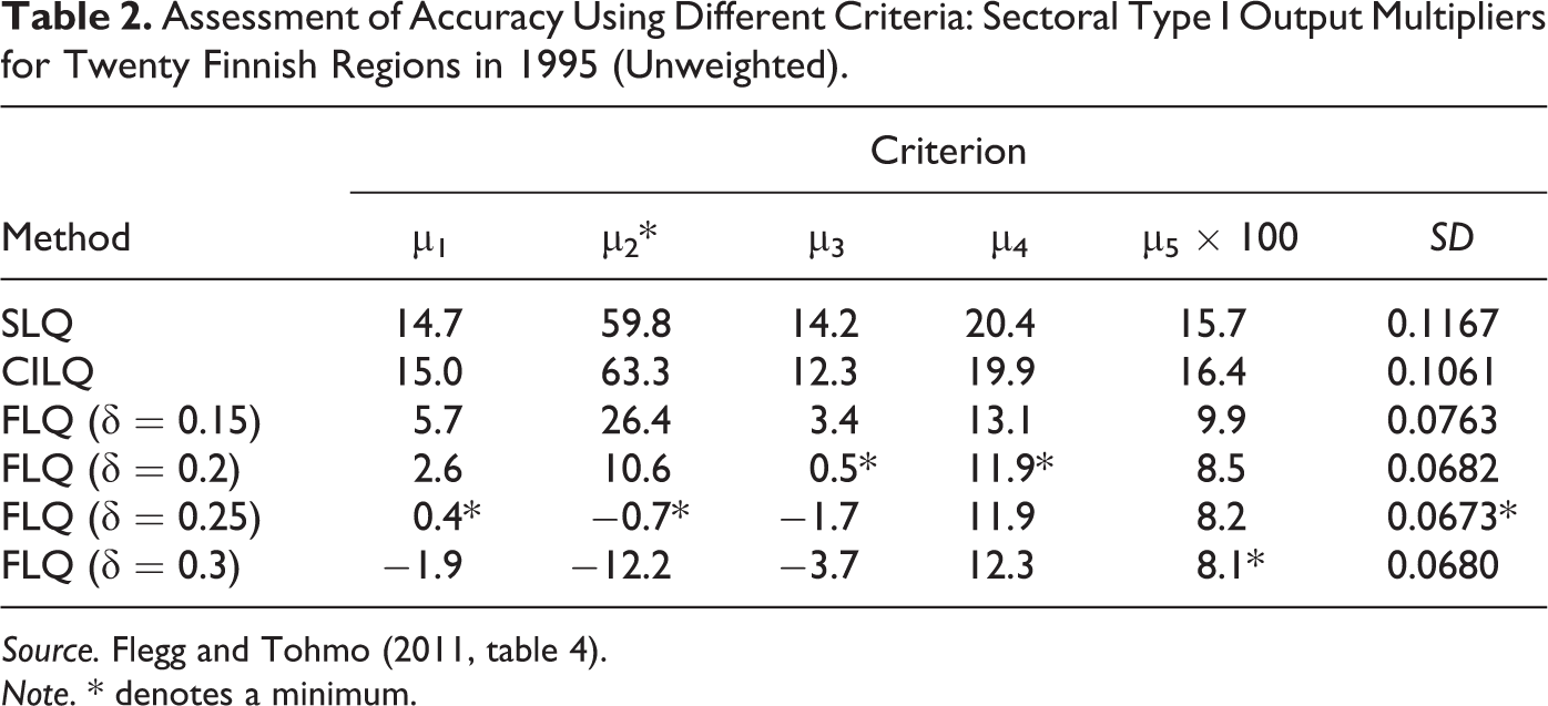
Source. Flegg and Tohmo (2011, table 4).

Note. * denotes a minimum.

Kronenberg’s Approach

Kronenberg eschews the use of LQs in favor of an approach based upon the resurrection and refinement of the classical commodity balance (CB) approach. A key issue for him is the way in which imports from abroad are allocated in national input−output tables. Here his use of type E tables as the basis for the application of his new approach is entirely appropriate since his aim is to capture the underlying technology of production. Let us now consider the salient differences between CHARM and the CB approach.

First note that the commodity balance for commodity i, b_i , is identical to net exports:

b_{i} \equiv e_{i} - m_{i},

where e and m denote exports and imports, respectively. The value of b_i is estimated by subtracting the estimated sum of intermediate and domestic final use of commodity i from an estimate of its output (Kronenberg 2009, 46). The CB method and CHARM yield exactly the same values of b_i but different values, in general, for the volume of trade, e_i + m_i. This is because CHARM takes cross-hauling into account. The amount of cross-hauling, q_i , is measured via the equation (ibid., 47):

q_{i} = (e_{i} + m_{i}) - | (e_{i} - m_{i}) |,

where (e_i + m_i ) is the volume and (e_i – m_i ) is the balance of trade, respectively. In the CB approach, q_i = 0 because e_i > 0 and m_i > 0 cannot, by assumption, occur simultaneously. By contrast, under Kronenberg’s approach, q_i > 0 is possible and, indeed, likely. He posits that q_i is proportional to the sum of the intermediate and domestic final use of commodity i, with the factor of proportionality being equal to the degree of product heterogeneity (ibid., 51).

Using data for the German state of North Rhine–Westphalia (NRW), Kronenberg computes supply multipliers for sixteen sectors. (Note. He refers to these as “output” multipliers but, to avoid confusion, we use the term supply multipliers.) As expected, the CB method yields unrealistically low figures for regional exports and imports, whereas CHARM generates more sensible figures for both (ibid., Table 3). However, even though the regional supply multipliers from CHARM are generally smaller than those for Germany, their average value is only marginally lower (1.553 vs. 1.590; ibid., Table 4). This suggests that CHARM may still be overestimating these multipliers, although it is true that NRW is a relatively large region (with around 21.7 percent of national employment).

Table 3.

Employees in Uusimaa and Finland by Regional Sector.

Sector	Description	Uusimaa: Employees (RE _i )	Finland: Employees (NE _i )	Regional Share (%)	National Share (%)	LQ _i
1	Agriculture and hunting (1)	3,409	104,000	0.5	4.4	0.104
2	Forestry and logging (2)	1,105	20,000	0.1	0.9	0.176
3	Fishing (3)	37	2,000	0.0	0.1	0.059
4	Mining and extraction (4−8)	635	6,000	0.1	0.3	0.336
5	Manufacture of food products, beverages and tobacco products (9−10)	9,462	41,000	1.3	1.7	0.733
6	Manufacture of textiles and clothes; dressing and dyeing of fur; tanning and dressing of leather; manufacture of luggage, handbags, saddlery, harness and footwear (11−13)	1,754	19,000	0.2	0.8	0.293
7	Manufacture of wood and of products of wood and cork, except furniture; manufacture of articles of straw and plaiting materials (14)	1,576	31,000	0.2	1.3	0.162
8	Manufacture of pulp, paper, and paper products; publishing, printing and reproduction of recorded media (15−16)	18,009	72,000	2.4	3.1	0.795
9	Manufacture of coke, refined petroleum products, nuclear fuels, chemicals and chemical products, rubber and plastic products (17−19)	9,127	40,000	1.2	1.7	0.725
10	Manufacture of other nonmetallic mineral products (20)	2,964	16,000	0.4	0.7	0.589
11	Manufacture of basic metals and fabricated metal products, other than machinery and equipment (21−22)	8,191	62,000	1.1	2.6	0.420
12	Manufacture of machinery and equipment not classified elsewhere (23)	10,460	63,000	1.4	2.7	0.527
13	Manufacture of office machinery and computers; electrical machinery and apparatus; radio, television and communication equipment and apparatus; medical, precision and optical instruments, watches and clocks (24−27)	26,823	66,000	3.6	2.8	1.291
14	Manufacture of motor vehicles, trailers, semi-trailers and other transport equipment (28−29)	5,986	25,000	0.8	1.1	0.761
15	Manufacture of furniture; manufacturing not classified elsewhere; recycling (30−31)	2,924	19,000	0.4	0.8	0.489
16	Electricity, gas, steam and hot water supply; collection, purification and distribution of water (32−33)	4,915	16,000	0.7	0.7	0.976
17	Construction (34)	42,555	155,000	5.8	6.6	0.872
18	Sale, maintenance, and repair of motor vehicles and motorcycles; retail of automotive fuel; wholesale, retail, and commission trade, excluding motor vehicles and motorcycles; repair of personal and household goods (35−37)	122,176	300,000	16.5	12.8	1.294
19	Hotels and restaurants (38)	27,228	77,000	3.7	3.3	1.123
20	Land, water, and air transport; travel agencies; post and telecommunications (39−43)	66,325	174,000	9.0	7.4	1.211
21	Financial intermediation; insurance and pension funding, except for compulsory social security (44−46)	20,733	41,000	2.8	1.7	1.606
22	Real estate and other business activities; rental of machinery and equipment and of personal and household goods; research and development (47−51)	114,585	236,000	15.5	10.0	1.542
23	Public administration and defense; compulsory social security (52)	52,838	173,000	7.1	7.4	0.970
24	Education (53)	50,405	157,000	6.8	6.7	1.020
25	Health and social work (54)	88,539	321,000	12.0	13.7	0.876
26	Sewage and refuse disposal, sanitation and similar activities; recreational, cultural, sporting and other service activities; private households with employed persons (55−59)	46,665	113,000	6.3	4.8	1.312
	Sum	739,426	2,349,000	100.0	100.0

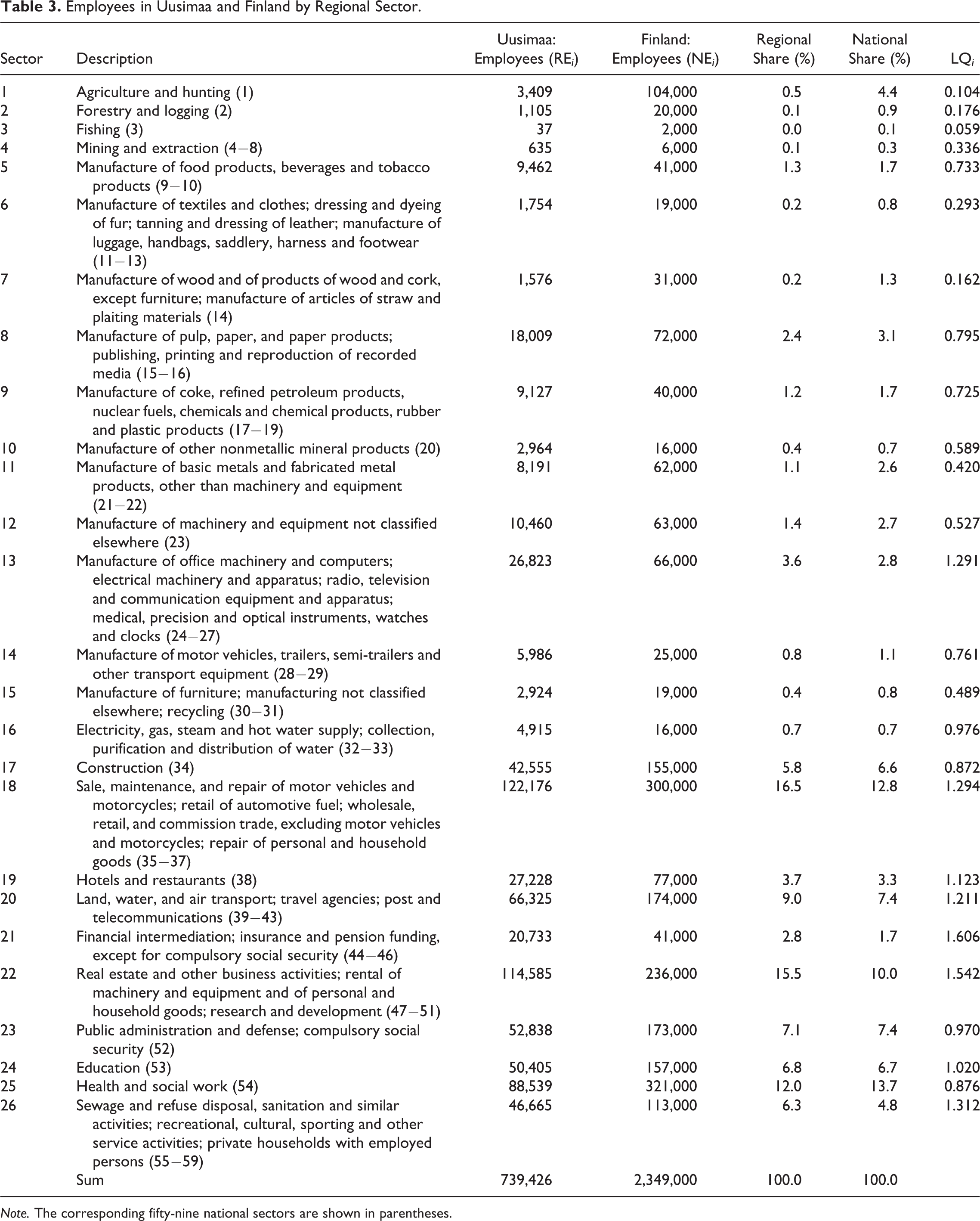
Note. The corresponding fifty-nine national sectors are shown in parentheses.

Table 4.

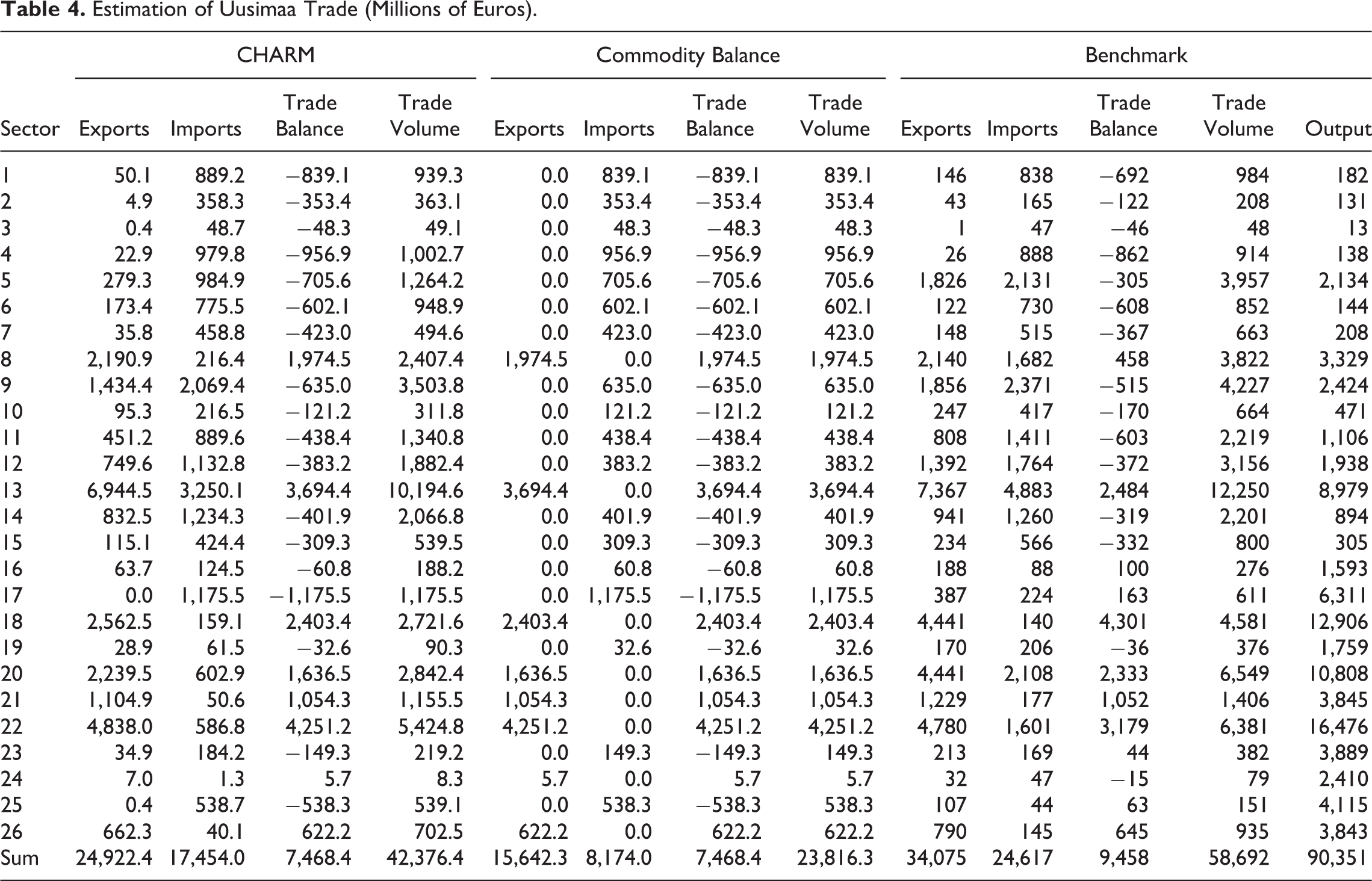
Estimation of Uusimaa Trade (Millions of Euros).

Sector	CHARM				Commodity Balance				Benchmark
Sector	Exports	Imports	Trade Balance	Trade Volume	Exports	Imports	Trade Balance	Trade Volume	Exports	Imports	Trade Balance	Trade Volume	Output
1	50.1	889.2	−839.1	939.3	0.0	839.1	−839.1	839.1	146	838	−692	984	182
2	4.9	358.3	−353.4	363.1	0.0	353.4	−353.4	353.4	43	165	−122	208	131
3	0.4	48.7	−48.3	49.1	0.0	48.3	−48.3	48.3	1	47	−46	48	13
4	22.9	979.8	−956.9	1,002.7	0.0	956.9	−956.9	956.9	26	888	−862	914	138
5	279.3	984.9	−705.6	1,264.2	0.0	705.6	−705.6	705.6	1,826	2,131	−305	3,957	2,134
6	173.4	775.5	−602.1	948.9	0.0	602.1	−602.1	602.1	122	730	−608	852	144
7	35.8	458.8	−423.0	494.6	0.0	423.0	−423.0	423.0	148	515	−367	663	208
8	2,190.9	216.4	1,974.5	2,407.4	1,974.5	0.0	1,974.5	1,974.5	2,140	1,682	458	3,822	3,329
9	1,434.4	2,069.4	−635.0	3,503.8	0.0	635.0	−635.0	635.0	1,856	2,371	−515	4,227	2,424
10	95.3	216.5	−121.2	311.8	0.0	121.2	−121.2	121.2	247	417	−170	664	471
11	451.2	889.6	−438.4	1,340.8	0.0	438.4	−438.4	438.4	808	1,411	−603	2,219	1,106
12	749.6	1,132.8	−383.2	1,882.4	0.0	383.2	−383.2	383.2	1,392	1,764	−372	3,156	1,938
13	6,944.5	3,250.1	3,694.4	10,194.6	3,694.4	0.0	3,694.4	3,694.4	7,367	4,883	2,484	12,250	8,979
14	832.5	1,234.3	−401.9	2,066.8	0.0	401.9	−401.9	401.9	941	1,260	−319	2,201	894
15	115.1	424.4	−309.3	539.5	0.0	309.3	−309.3	309.3	234	566	−332	800	305
16	63.7	124.5	−60.8	188.2	0.0	60.8	−60.8	60.8	188	88	100	276	1,593
17	0.0	1,175.5	−1,175.5	1,175.5	0.0	1,175.5	−1,175.5	1,175.5	387	224	163	611	6,311
18	2,562.5	159.1	2,403.4	2,721.6	2,403.4	0.0	2,403.4	2,403.4	4,441	140	4,301	4,581	12,906
19	28.9	61.5	−32.6	90.3	0.0	32.6	−32.6	32.6	170	206	−36	376	1,759
20	2,239.5	602.9	1,636.5	2,842.4	1,636.5	0.0	1,636.5	1,636.5	4,441	2,108	2,333	6,549	10,808
21	1,104.9	50.6	1,054.3	1,155.5	1,054.3	0.0	1,054.3	1,054.3	1,229	177	1,052	1,406	3,845
22	4,838.0	586.8	4,251.2	5,424.8	4,251.2	0.0	4,251.2	4,251.2	4,780	1,601	3,179	6,381	16,476
23	34.9	184.2	−149.3	219.2	0.0	149.3	−149.3	149.3	213	169	44	382	3,889
24	7.0	1.3	5.7	8.3	5.7	0.0	5.7	5.7	32	47	−15	79	2,410
25	0.4	538.7	−538.3	539.1	0.0	538.3	−538.3	538.3	107	44	63	151	4,115
26	662.3	40.1	622.2	702.5	622.2	0.0	622.2	622.2	790	145	645	935	3,843
Sum	24,922.4	17,454.0	7,468.4	42,376.4	15,642.3	8,174.0	7,468.4	23,816.3	34,075	24,617	9,458	58,692	90,351

Case Study of Uusimaa

A limitation of Kronenberg’s case study is that he did not have the benchmark regional data needed to assess the accuracy of his CHARM-based estimates of imports, exports, and multipliers. Fortunately, in the case of Finland, the necessary figures can be derived for all its regions in 2002.⁴ Here we examine data for Uusimaa, the largest region, which produced 34.6 percent of national output in 2002 and accounted for 31.4 percent of aggregate employment. Uusimaa’s diversified industrial structure is illustrated in Table 3.

It should be noted that we have pursued a more disaggregated approach than Kronenberg did, so as to maximize the amount of available information and minimize aggregation bias. Even so, a lack of regional data meant that the fifty-nine national sectors had to be reduced to the twenty-six regional sectors displayed in Table 3.⁵ In evaluating the relative performance of CHARM and the CB method, we use the regional data generated by Statistics Finland as a benchmark.

Table 5.

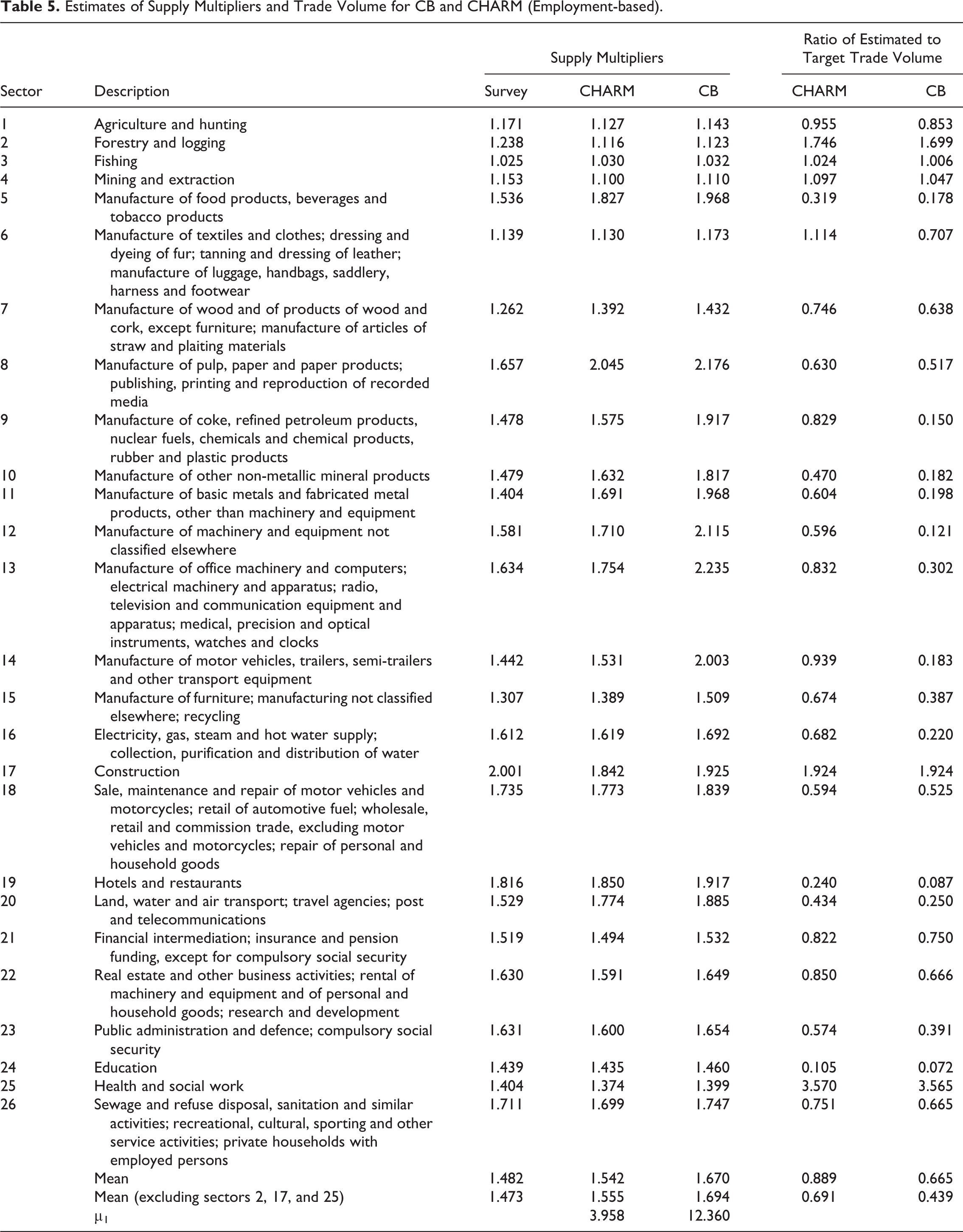
Estimates of Supply Multipliers and Trade Volume for CB and CHARM (Employment-based).

Sector	Description	Supply Multipliers			Ratio of Estimated to Target Trade Volume
Sector	Description	Survey	CHARM	CB	CHARM	CB
1	Agriculture and hunting	1.171	1.127	1.143	0.955	0.853
2	Forestry and logging	1.238	1.116	1.123	1.746	1.699
3	Fishing	1.025	1.030	1.032	1.024	1.006
4	Mining and extraction	1.153	1.100	1.110	1.097	1.047
5	Manufacture of food products, beverages and tobacco products	1.536	1.827	1.968	0.319	0.178
6	Manufacture of textiles and clothes; dressing and dyeing of fur; tanning and dressing of leather; manufacture of luggage, handbags, saddlery, harness and footwear	1.139	1.130	1.173	1.114	0.707
7	Manufacture of wood and of products of wood and cork, except furniture; manufacture of articles of straw and plaiting materials	1.262	1.392	1.432	0.746	0.638
8	Manufacture of pulp, paper and paper products; publishing, printing and reproduction of recorded media	1.657	2.045	2.176	0.630	0.517
9	Manufacture of coke, refined petroleum products, nuclear fuels, chemicals and chemical products, rubber and plastic products	1.478	1.575	1.917	0.829	0.150
10	Manufacture of other non-metallic mineral products	1.479	1.632	1.817	0.470	0.182
11	Manufacture of basic metals and fabricated metal products, other than machinery and equipment	1.404	1.691	1.968	0.604	0.198
12	Manufacture of machinery and equipment not classified elsewhere	1.581	1.710	2.115	0.596	0.121
13	Manufacture of office machinery and computers; electrical machinery and apparatus; radio, television and communication equipment and apparatus; medical, precision and optical instruments, watches and clocks	1.634	1.754	2.235	0.832	0.302
14	Manufacture of motor vehicles, trailers, semi-trailers and other transport equipment	1.442	1.531	2.003	0.939	0.183
15	Manufacture of furniture; manufacturing not classified elsewhere; recycling	1.307	1.389	1.509	0.674	0.387
16	Electricity, gas, steam and hot water supply; collection, purification and distribution of water	1.612	1.619	1.692	0.682	0.220
17	Construction	2.001	1.842	1.925	1.924	1.924
18	Sale, maintenance and repair of motor vehicles and motorcycles; retail of automotive fuel; wholesale, retail and commission trade, excluding motor vehicles and motorcycles; repair of personal and household goods	1.735	1.773	1.839	0.594	0.525
19	Hotels and restaurants	1.816	1.850	1.917	0.240	0.087
20	Land, water and air transport; travel agencies; post and telecommunications	1.529	1.774	1.885	0.434	0.250
21	Financial intermediation; insurance and pension funding, except for compulsory social security	1.519	1.494	1.532	0.822	0.750
22	Real estate and other business activities; rental of machinery and equipment and of personal and household goods; research and development	1.630	1.591	1.649	0.850	0.666
23	Public administration and defence; compulsory social security	1.631	1.600	1.654	0.574	0.391
24	Education	1.439	1.435	1.460	0.105	0.072
25	Health and social work	1.404	1.374	1.399	3.570	3.565
26	Sewage and refuse disposal, sanitation and similar activities; recreational, cultural, sporting and other service activities; private households with employed persons	1.711	1.699	1.747	0.751	0.665
	Mean	1.482	1.542	1.670	0.889	0.665
	Mean (excluding sectors 2, 17, and 25)	1.473	1.555	1.694	0.691	0.439
	μ₁		3.958	12.360

As expected, Table 4 shows that the CB method substantially underestimates Uusimaa’s total exports and imports and, consequently, its volume of trade. CHARM performs markedly better, although it too understates the overall amount of trade. This superior relative performance is primarily due to the fact that CHARM takes cross-hauling into account, whereas the CB method rules out the possibility of a sector’s being both an exporter and an importer of a given commodity.

From Table 5, we can see that CHARM almost invariably produces the best estimates of the volume of trade in individual sectors. This pattern is especially noticeable with respect to manufacturing (sectors 5 to 15), where it can be explained by the heterogeneity of many manufactured products and the concomitant cross-hauling. Sector 13 is a good example: whereas CHARM captures 83.2 percent of the volume of trade, the CB method accounts for only 30.2 percent. Furthermore, the more detailed results in Table 4 reveal that CHARM captures almost all of the exports in sector 13 and two-thirds of the imports; by contrast, the CB method accounts for half of the exports but none of the imports.

The differences between CHARM and the CB method are generally less striking for the nonmanufacturing sectors. We should not expect cross-hauling to be an issue for many service industries, so CHARM is unlikely to outperform the CB method. Indeed, both methods perform very poorly indeed in the sectors Hotels and Restaurants (19) and Education (24), even though the amount of trade involved is modest. Furthermore, there are three sectors (2, 17, and 25) where both methods dramatically overstate the volume of trade and by comparable amounts. This problem can, in turn, be attributed to errors in estimating the balance of trade, b_i , which equals net exports. Table 4 records estimates for b_i of –353.4, –1,175.5, and –538.3 (× €1 million) for sectors 2, 17, and 25, respectively, which are not at all like the corresponding target figures of –122, 163, and 63. In the case of Construction (sector 17), the error is due to the fact that the intermediate and final demands for construction were overestimated by 6.5 percent and 7.8 percent, respectively, while output was underestimated by 14.0 percent. For Health and Social Work (sector 25), the error can be attributed a 10.4 percent overstatement of final demand and a 4.9 percent understatement of output. Finally, for Forestry and Logging (sector 2), output was overstated by 24.8 percent but this error was dwarfed by the fact that the intermediate and final demands for this sector’s output were overestimated by 97.9 percent and 120.6 percent, respectively.

It should be noted that we followed Kronenberg in making certain assumptions in our calculations of sectoral output and demand. In particular, we used employment data as a proxy for output. This is likely to be problematic in cases where there is a significant divergence between regional and national labor productivity. We also assumed identical national and regional technology. Finally, in calculating the regional final use of each commodity, we simply used the ratio of total regional to total national employment to scale down the national figures (cf. Kronenberg 2009, 46).

Figure 1 highlights the fact that, almost invariably, the CB method substantially underestimates the volume of Uusimaa’s imports. CHARM generally performs much better, although it does still often understate the volume of imports. This understatement is especially noticeable for sectors 5, 8, 13, 20, and 22. On the other hand, both methods substantially overstate imports for sectors 17 and 25.

Figure 1.

Estimates of imports for CB and CHARM.

Turning now to the estimates of supply multipliers in Table 5, we can see that both methods typically overstate the size of these multipliers, although CHARM comes much closer to the target on average. CHARM is invariably the better method for manufacturing (sectors 5 to 15), but the pattern is less clear-cut for the nonmanufacturing sectors. For instance, the CB method generates the closest estimates for Construction (17) and Health and Social Work (25). Nevertheless, in terms of the mean proportional error, μ₁, as defined in equation (16), it is clear that CHARM is by far the more accurate of the two methods: it yields an average error of 4.0 percent versus 12.4 percent for the CB method.

To shed some light on the possible causes of these errors, we reworked our results using production rather than employment data. As expected, accuracy improved, yet most of the error remained. In particular, μ₁ fell to 3.0 percent for CHARM and to 10.4 percent for the CB method. The limited extent of this improvement is due to the fact that labor productivity in Uusimaa is typically not very different from that in Finland. This outcome can, in turn, be attributed to Uusimaa’s predominance in the Finnish economy. In other regions, especially those that are relatively small and located far from Helsinki, the differences between national and regional labor productivity are likely to be more pronounced and the consequences more substantial.

Conclusion

Kronenberg has produced an innovative, rigorous, and usable refinement of the classical CB method. Moreover, his proposed new method (CHARM) is firmly grounded in economic theory. Kronenberg did not, however, possess the benchmark regional data required to validate CHARM, so the principal aim of this comment has been to subject it to a detailed empirical test. Our test used data for Uusimaa, Finland’s largest region, produced by Statistics Finland. We were able to assess the accuracy of the estimates of exports, imports, volume of trade, balance of trade, and supply multipliers generated by CHARM and the CB method for twenty-six regional sectors in 2002. We found that CHARM outperformed the CB method in all important respects. The results were particularly encouraging for manufacturing sectors, which typically produce heterogeneous commodities and where cross-hauling is rife.

Our findings in terms of supply multipliers are especially worth noting. A tendency toward overstatement of regional multipliers is a well-known characteristic of non-survey techniques, yet CHARM performed well in this respect: on average across the twenty-six sectors, the unweighted mean supply multiplier from CHARM was 1.542, which is not far above the target figure of 1.482. By comparison, the CB method generated a mean of 1.670. What is more, the mean proportional error from CHARM was 4.0 percent, which compares very favorably with the 12.4 percent from the CB method.

CHARM is based on a relatively new type of national input−output table, in which imports from abroad are incorporated into the interindustry transactions matrix, so that the input coefficients derived from this matrix are genuine technical coefficients. We refer to tables of this kind as type A tables. Such tables are produced by all members of the EU (and by some other countries too). However, Kronenberg fails to mention that EU countries also produce a more traditional type of national table, from which imports from abroad are excluded. We refer to tables of that kind as type B tables. In our comment, we attempt to clarify the differences between these two types of table and then explore the implications. We aver that Kronenberg is right to employ type A tables in the context of CHARM. However, where LQs are being used to regionalize a national table, we argue that there are compelling reasons for applying the LQs to type B tables. Furthermore, of the possible LQs that might be used, we maintain that there are strong theoretical and empirical grounds for using the FLQ.⁶

Kronenberg does not consider possible regional applications for which CHARM, as opposed to LQs, would be suitable. To clarify this issue, suppose that an analyst is interested in the impact of the expansion of a coal-fired power station in a particular region. If he is interested specifically in the environmental effects of burning more coal, then the source of the coal inputs would be irrelevant. In this instance, we would recommend using CHARM to regionalize the type A national table. The resulting regional table could then be employed to estimate supply multipliers. If, on the other hand, the analyst’s focus is on regional output and employment, then we would suggest using the FLQ to regionalize the type B national table. The resulting regional table could then be used to compute output and employment multipliers.

The results obtained here for Uusimaa are certainly encouraging in terms of the effectiveness of CHARM as a regionalization method in situations where type A regional tables are most appropriate. However, one should always be cautious in generalizing from the findings of a case study of a single region. For this reason, we repeated our analysis for a further eleven Finnish regions, which varied in terms of their characteristics. We found that CHARM invariably outperformed the CB method in these regions as well, and by a wide margin. However, the estimates generated by CHARM for these other regions were substantially less accurate than those obtained for Uusimaa. A possible explanation of this finding is that it is due to a greater divergence between regional and national labor productivity in these other regions. This hypothesis suggests that it might be fruitful to attempt to make some adjustment for differences in productivity when using CHARM to construct regional input–output tables. It is also worth pursuing the reasons why CHARM consistently overstated the size of the supply multipliers, both in Uusimaa and in the other regions we examined.

Footnotes

Acknowledgment

The authors would like to thank Tobias Kronenberg for clarifying several points regarding the application of CHARM. Helpful comments were received from Andrew Mearman, Anthony Plumridge, Chris Webber, and Don Webber.

Declaration of Conflicting Interests

The author(s) declared no potential conflicts of interest with respect to the research, authorship, and/or publication of this article.

Funding

The author(s) received no financial support for the research, authorship, and/or publication of this article.

Notes

References

Bonfiglio

Chelli

. 2008. “Assessing the Behaviour of Non-survey Methods for Constructing Regional Input−Output Tables through Monte Carlo Simulation.” Economic Systems Research 20:243–58.

Boomsma

Oosterhaven

. 1992. “A Double-entry Method for the Construction of Bi-regional Input–Output Tables.” Journal of Regional Science 32:269–84.

Flegg

A. T.

Tohmo

. 2011. “Regional Input–Output Tables and the FLQ Formula: A Case Study of Finland.” Regional Studies, first published on August 25, 2011 (iFirst) doi:10.1080/00343404.2011.592138

Flegg

A. T.

Webber

C. D.

Elliott

M. V.

. 1995. “On the Appropriate Use of Location Quotients in Generating Regional Input–Output Tables.” Regional Studies 29: 547–61.

Flegg

A. T.

Webber

C. D.

. 1997. “On the Appropriate Use of Location Quotients in Generating Regional Input–Output Tables: Reply.” Regional Studies 31:795–805.

Flegg

A. T.

2000. “Regional Size, Regional Specialization and the FLQ Formula.” Regional Studies 34:563–69.

Hewings

G. J. D.

Jensen

R. C.

. 1986. “Regional, Interregional and Multiregional Input–Output Analysis.” In Handbook of Regional and Urban Economics, vol. I, ed. Nijkamp

, 295–355. Amsterdam, Netherlands: Elsevier.

Kronenberg

. 2009. “Construction of Regional Input–Output Tables using Nonsurvey Methods: The Role of Cross-hauling.” International Regional Science Review 32:40–64.

Kronenberg

. 2011. “Regional Input–Output Models and the Treatment of Imports in the European System of Accounts.” MPRA Paper No. 30797, online at http://mpra.ub.uni-muenchen.de/30797/ and forthcoming in Jahrbuch für Regionalwissenschaft. doi: 10.1007/s10037-012-0065-2.

10.

Louhela

2006. “Estimation of Interregional Trade for Finnish Regions in 1996 and 2002—Freight Flow and Gravity Approaches.” Paper presented at the 46th Congress of the European Regional Science Association, Velos, Greece, August 30–September 3, 2006.

11.

Riddington

Gibson

Anderson

. 2006. “Comparison of Gravity Model, Survey and Location Quotient-based Local Area Tables and Multipliers.” Regional Studies 40:1069–81.

12.

Robison

M. H.

Miller

J. R.

. 1988. “Cross-hauling and Nonsurvey Input–Output Models: Some Lessons from Small-area Timber Economies.” Environment and Planning A 20:1523–30.

13.

Statistics Finland. 2000. Regional Input–Output 1995: Tables and Compilation Methods. Helsinki: Official Statistics of Finland.

14.

Tohmo

. 2004. “New Developments in the Use of Location Quotients to Estimate Regional Input–Output Coefficients and Multipliers.” Regional Studies 38:43–54.

15.

United Nations. 1973. Input–Output Tables and Analysis. New York: United Nations.

16.

West

G. R

. 1990. “Regional Trade Estimation: A Hybrid Approach. International Regional Science Review 13: 103–118.