
Abstract
The vector assignment p-median problem (VAPMP) and the ordered p-median problem (OMP) are important extensions of the classic p-median problem. The VAPMP extends the p-median problem by allowing assignment of a demand to multiple facilities, and a wide variety of multi-assignment and backup location problems are special cases of this problem. The OMP optimizes a weighted sum of service distances according to their relative ranks among all demands. The OMP is well known as it represents a generalization of both the p-median and the p-center problems. In this article, a new model is developed which extends both the VAPMP and OMP problems. In addition, beyond median, center, and vector assignment, this new model can resolve problems where the system objective involves maximizing distance. The new model also gives rise to meaningful special-case problems, such as a “reliable p-center” problem. Different integer linear programming (ILP) formulations of the new problem are presented and tested. It is demonstrated that an efficient formulation for a special case of the VAOMP problem can solve medium sized problems optimally in a reasonable amount of time.
Keywords
Introduction
Location analysis has been an area of active research over the past four decades. Powered by the development in optimization techniques, mathematical programming, computational theory, algorithms, and computer hardware, the domain of location analysis has been greatly expanded. A large number of models and problems involving different criteria and constraints have been developed, in an attempt to capture to a greater extent the complexity of the real world. There is a general consensus in the location science literature (see e.g., reviews by Brandeau and Chiu 1989; Owen and Daskin 1998; ReVelle and Eiselt 2005; Daskin 2008) that there are four basic types of models, namely, the p-median problem, the simple plant location problem (SPLP), the p-center problem and covering problems (including the location set covering problem (LSCP) and the maximal covering location problem [MCLP]). There are other location problems that have appeared in the literature that are distinctively different from the four basic models in terms of their objectives and structures. These include, for example, undesirable or obnoxious facility location, facility dispersion, facility interdiction problems, location with backup service, unreliable facility location, and the hub location problem. Moreover, there are many extensions of location models in the sense that they can be added to a basic location model as the specific application context requires. A well-known example is the addition of capacity conditions to the SPLP. Another fundamental yet often neglected example is the protocol or rule for assigning individual demands to routes or service facilities in location analysis. A common protocol, called the closest assignment (CA) condition, is that each demand will be assigned to the closest facility or least cost route for service from the facility. Whether this condition is incorporated into a modeling framework or not largely distinguishes the purpose between user-oriented models and system optimal models.
Despite the multitude of location problems and extensions that have been developed, it is possible, in some occasions to unify basic location problems that appear to be drastically different. Even though it may be impossible to devise one problem to model the infinite complexity of the real world, the unification of different location models is important because (1) it helps in the classification and the understanding of the connections between different problems and (2) it often provides a means to identify and construct new models to meet the needs of analysis. In certain occasions, it is even possible to develop a unified means for solving a variety of related problems in a relatively efficient manner.
One of the earliest examples of model unification in location analysis is the work of Church and ReVelle (1976) in which the authors identified theoretical and computational links between the p-median problem and covering problems. In a similar vein, Hillsman (1984) proposed to use the p-median structure to solve a variety of location problems by appropriately modifying the distance or cost matrix. Weaver and Church (1985) developed the Vector Assignment p-median problem (VAPMP) which allowed split and multiple assignments. The weight values for making assignments to different facilities are based upon the relative closeness of the facilities for a given demand. Further, Church and Weaver (1986) showed that the VAPMP can be used to structure a variety of expected coverage and multilevel covering problems. In essence, it was shown that a number of single-level and multilevel cover models were special cases of the VAPMP.
A prominent recent development is the Ordered Median Problem (OMP; Nickel and Puerto 1999), which is well known for its ability to generalize the p-median and p-center problems as well as define new problems based on the order of the demands in terms of their closest service distance or lowest cost.1 Whereas the VAPMP is based upon modeling the order of facility closeness for each demand, the OMP problem is based upon ordering demand in terms of service by their respective closest facility. At first this distinction appears to be quite subtle, but a closer look will reveal that these two model approaches are quite different; while the OMP deals with the single level CA, the VAPMP deals with multilevel CA for each demand.
The goal of this article is to introduce a new location model called the Vector Assignment Ordered Median Problem (VAOMP). VAOMP generalizes both the VAPMP and the OMP. Moreover, it is designed to be sensitive to distance in terms of facility or route choice. Consequently, problems such as obnoxious facility location and facility interdiction can be posed in terms of the new model, when negative weights are used. The new model not only subsumes some of the recently developed location models as special case problems but helps identify new location problems. For example, it is possible to formulate a “reliable p-center problem” using the VAOMP structure.
The rest of this article is organized as follows. The next section reviews the VAPMP and the OMP as well as past work to provide motivation for developing the VAOMP. Then, a subsequent section presents several alternative integer linear programming (ILP) formulations of the VAOMP. Following that, we provide specific examples of meaningful special case problems of the new VAOMP model. The experiments section presents computational results using two different data sets. Finally, we conclude with a summary of findings and needed future work.
Background and Motivation
Historically, research in location modeling was inspired by private sector applications with the Weber problem and its extensions, and the SPLP (Manne 1964; Balinski 1965). As pointed out by ReVelle, Marks, and Liebman (1970), location analysis in the public sector involves the added complexity that objectives and constraints are not as easily quantified or defined. They classified public location sector problems into two categories, ordinary and emergency services. In the former case, average travel time or distance in being served by the closest facility is often used as a surrogate or substitute measure for utility. In the latter, a maximum acceptable travel distance or time is often used as standard for service. Depending on whether the maximum distance is minimized or used as a fixed upper-bound or distance standard, two additional problems types can be defined, namely, center location problems and the covering location problems (including the LSCP [Toregas et al. 1971] and the MCLP [Church and ReVelle 1974]). These two problem types plus the p-median and the SPLP problem constitute what is generally recognized as the four fundamental problems in the location science literature. Based on these fundamental location problems, various extended problems have been developed, as will be discussed later in this section.
It is somewhat surprising that even the basic location problems can be related to each other structurally. One of the earliest efforts in identifying such connections is the work of Church and ReVelle (1976) who showed a relationship between covering and median problems. A more recent example is the OMP (Nickel and Puerto 1999) which provided a general structure to unify the p-median and p-center problems.
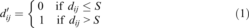
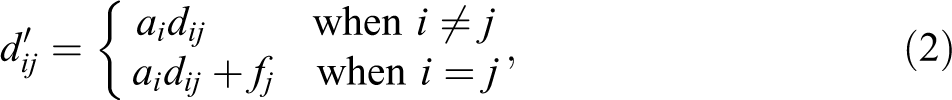
Church and ReVelle (1976) established that covering location problems such as the MCLP can be posed as a p-median problem via the following transformation of the distance or cost matrix:
where i is an index of demand, j is an index of facility sites,
where
where
Another major generalization of the p-median location problem is the OMP (Nickel and Puerto 1999; Kalcsics et al. 2002; Domínguez-Marín et al. 2005; Nickel and Puerto 2005; Puerto and Tamir 2005; Boland et al. 2006; Stanimirović, Kratica, and Dugošija 2007; Marín et al. 2009). The main advantage of the OMP is that it is a general structure that can unify the p-median problem and the p-center problem, as well as represent intermediate hybrid problems between median and center problems. This is achieved by putting a vector
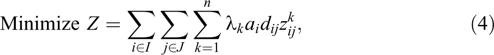
An ILP formulation of the OMP (due to Boland et al. [2006]) can be given as follows:
s.t.

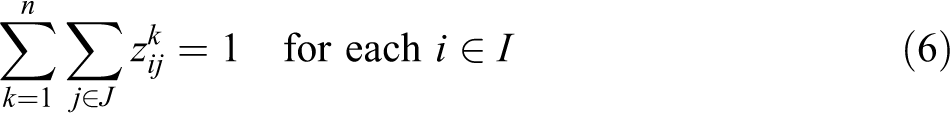

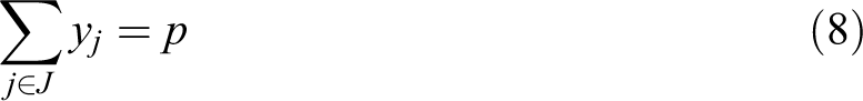

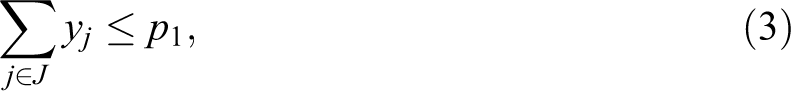
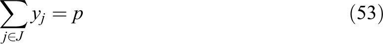
In this formulation, objective (4) minimizes the sum of weighted distances (product of demand times distance), each further weighted by the λ vector according to their relative service ranks. Constraint (5) maintains that, at each service rank k, only one demand assignment can be made. Constraint (6) requires that each demand i is assigned exactly one service rank as well as assigned to only one facility. Constraints (5) and (6) together maintain that each demand assigns once to a facility, there is only one demand assigned to a given service rank, and all demands are assigned a service rank. Constraint (7) maintains the order of the service ranks based upon the distance associated with the assignment. For example, if a demand i is assigned a rank of 4 at a distance of 100, then the demand which is assigned a rank of 5 must have a distance that equals or exceeds 100. Constraint (8) establishes that exactly p-facilities will be located. Constraint (9) is an expanded form of a Balinski style constraint that maintains that assignment for any service rank cannot be made to a site unless that site has been selected for a facility. When all
Extending the work of Nickel and Puerto (1999), Kalcsics et al.(2002) identified finite optimality sets for the single facility problem involving different sets of weight vectors λ and derived results on computational complexity. Puerto and Tamir (2005) considered a variant of OMP for locating tree-shaped facilities on a tree network. Drezner and Nickel (2009a, 2009b) developed solution procedures for solving the single facility OMP on the continuous plane. Heuristic procedures for the OMP, such as genetic algorithms and variable neighborhood search, were investigated by Domínguez-Marín, et al.(2005) and Stanimirović, Kratica, and Dugošija (2007). Boland et al.(2006) investigated exact solution procedures for solving the discrete OMP as well as developed branch and bound procedures for solving the discrete OMP. They suggested alternative ILP formulations for the OMP problem and tested different measures for improving the formulation, such as using externally determined bounds, variable fixing as well as adding valid inequalities. Marín et al. (2009) presented an alternative formulation of the OMP (based on pre-sorted distances) as well as a specialized branch and cut procedure. For a systematic treatment of the OMP, the reader is referred to a book by Nickel and Puerto (2005) and a book by Domínguez-Marín (2003).
One of the potential issues of OMP formulations such as (4) through (9) pertains to the protocol for assigning demands to facilities. Normally, the λ vector is nonnegative, which makes the OMP “distance minimizing” just as the classic p-median problem. One can potentially set the λ vector to negative values to model obnoxious facility location or hostile interdiction of facilities. In a model for locating obnoxious facilities, the system will try to maximize the distance from each demand to its closest facility. The facility interdiction problem (Church, Scaparra, and Middleton 2004) aims at identifying critical facilities which, if removed, will result in maximizing total distance traveled by the demands. In both occasions, despite the fact the system objective is “distance maximizing,” each demand should still be assigned to its closest facility. This assignment protocol is called CA and it will be violated unless explicit constraints are imposed.
With the above discussion in mind, the goal of this article is to develop a new unified median location problem which we call the VAOMP. It is a generalization of both the VAPMP and the OMP, and therefore generalizes a multitude of classic location problems each of them generalizes. In addition, the new model allows one to define new location constructs such as a “reliable” p-center problem, which will be discussed in a subsequent section. Furthermore, the new model is formulated with explicit CA conditions. This makes the new model suitable for locating obnoxious facilities, something not possible with existing formulations of the OMP.
Formulating VAOMP
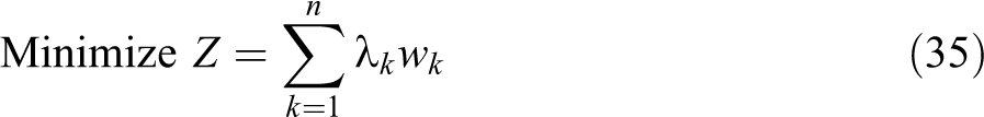
This section presents several ILP formulations of the VAOMP. The Vector Assignment Median problem involves assigning a demand to its first closest facility for some fraction of its needs, a second closest facility for an additional fraction of its need, and so on, whereas the OMP assigns each demand to its closest facility, but keeps track of which demand gets the closest or best service, which demand gets the second best service, and so on. In combining these two constructs, we need to allow multiple assignments for each demand as well as rank the level of combined service, in terms of which demand receives the best combined level of service, which demand receives the next best level of combined service, and so on. The generalized model will then minimize the weighted combined service levels, based upon the weight vector λ. To formulate this model, we need to introduce or refine the definitions of the following terms:
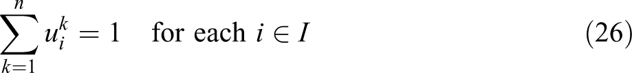
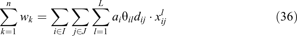
To describe the VAOMP objective, we need to describe for each demand i, the (weighted) partial sum of service distances (to its closest L facilities). We call this a weighted partial sum, as it is a sum of distances to only the L closest facilities, each weighted by the service fraction (or service weight) to that facility. Then, the (weighted) sum of the partial sums defines the VAOMP objective. Recall that index k defines an ordering among the costs for serving the demands, whereas index l is used to identify the ordering of the facilities in terms of distance to a specific demand i. A straightforward formulation of the VAOMP can be written in terms of the following assignment variable:

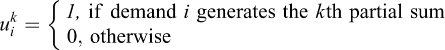
Other necessary decision variables are:


With the above notation, the VAOMP can be formulated as follows (which we call VAOMP_A to indicate the fact that this formulation uses assignment variables):
VAOMP_A:
s.t.
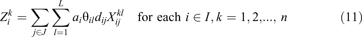


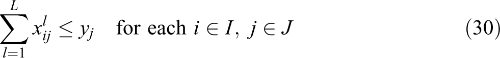
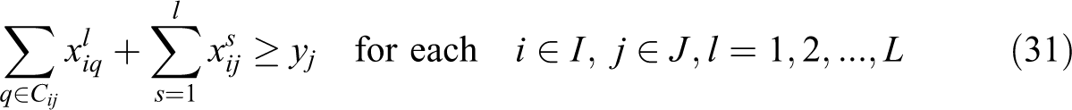
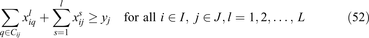
In this formulation, constraint (11) defines the weighted partial sum of distances for each demand i, in terms of assignment variables
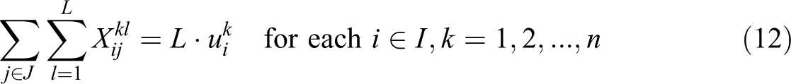
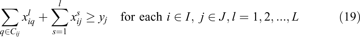
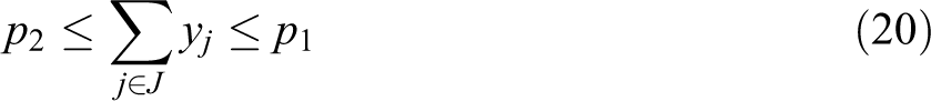
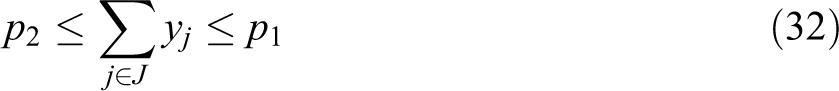
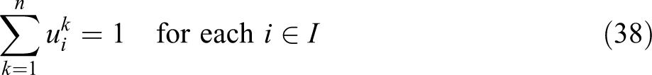
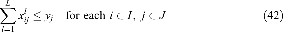
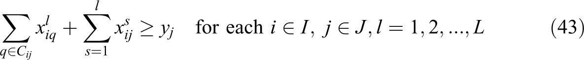
Constraints (19) ensure that a given demand
Constraint (21) defines the appropriate ranges and restrictions for the decision variables. Note that the binary requirement of the assignment variables can be relaxed because when appropriate forms of MLCA such as (19) are used, the assignment variables will be forced to integer values even if they are defined as continuous variables. A more detailed discussion of this property can be found in Lei and Church (2011a).
The VAOMP_A formulation uses an assignment variable
VAOMP_H:
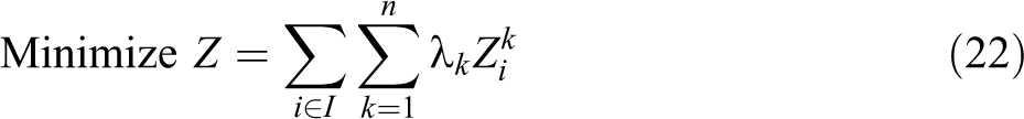
s.t.

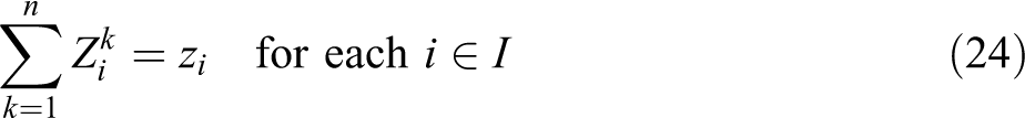


The VAOMP_H formulation is similar in structure to VAOMP_A. In fact, constraints (26) through (32) are the same with constraints (13), (14), (15), (17), (18), (19), and (20). What is different from the VAOMP_A formulation is that constraint (23) defines the partial sum at demand

Compared with VAOMP_A, the VAOMP_H formulation has a significantly reduced number of variables and constraints. This is achieved by structuring constraints (23), (24) and (25) based on “unconditional” partial sums at each demand

VAOMP_H2:
s.t.


In this formulation, constraint (36) is written in terms of the unconditional partial sum
It is worthy to note that some constraints in the above VAOMP formulations can be omitted when the parameters of the problem meet certain conditions. First of all, if

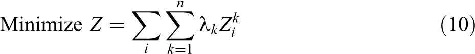
Basically, this inequality means that for all possible permutations of two sequences, the inner product of the two permutations will be the smallest when they have opposite orders and will be the greatest if they have the same order. Applying this to the VAOMP objective function (10), we can see that if
Second, when the assignment vector θ
has non-increasing entries and the λ vector is nonnegative, the (multilevel) CA constraint (19) is optional. This can be proved using a similar argument using the Hardy-Littlewood-Pólya inequality. The above two properties hold regardless of whether
Finally, if the ranking vector λ is non-decreasing, that is,

The special-case formulation which we call VAOMP_C is as follows:
VAOMP_C:


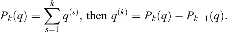
The above formulation makes use of the linear programming formulation of Ogryczak and Tamir (2003) to minimize the sum of the k largest numbers in an array. Their article showed that the sum of the k largest numbers in an array
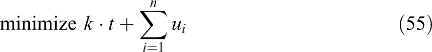


A formal proof can be found in Ogryczak and Tamir’s paper. Intuitively, the validity of this program can be verified by the following reasoning. Let
Using a similar argument as Ogryczak and Tamir (2003), but with slightly different notation, let the k largest elements of an array
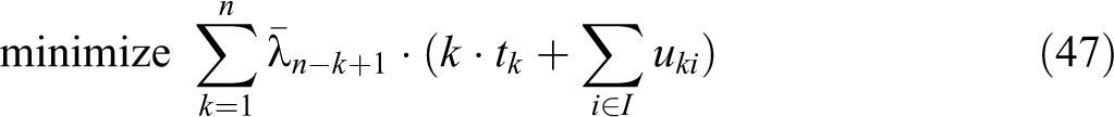
The VAOMP objective (47) can be rewritten as
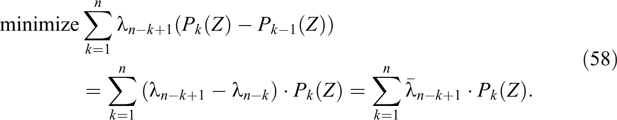
Using (55) through (57), we have:

We can substitute (59) into (58). When
Observation
The VAOMP_C formulation (47) through (54) is a valid formulation of VAOMP when the rank vector λ is nonnegative and weakly increasing.
Applications and special cases of VAOMP
The previous section presented several formulations for the VAOMP problem. In this section, we provide some examples of location problems for which the VAOMP problem can be used as a unified model. Before we discuss specific cases, there are several general issues that are important to mention. First, although the assignment vector in the original VAPMP problem was meant to represent the portions or probabilities of a demand being served by multiple facilities, they can in general represent any meaningful weight values associated with assignment at each level of closeness. For example, this was used in Church and Weaver (1986) to formulate the BACOP (Hogan and ReVelle 1986) in which each demand is required to be covered by different facilities a given number of times. As another example, the assignment vector can represent a combination of probability and a penalty for a demand in using backup facilities or backup routes. As pointed out by Snyder and Daskin (2005), the transportation cost for using backup facilities can be higher than the normal cost. For a risk aversive management strategy, it may be necessary to put a high penalty on using backup facilities.
Second, we note that negative weights in the objective (i.e., the assignment vector or the rank vector) can be used in certain applications when the system objective is “distance maximizing.” For one example, the location of obnoxious facilities (Church and Garfinkel 1978) can involve placing undesirable facilities as far away from population centers as possible. In this occasion, explicit constraints for CA are needed because it is the closest undesirable facility that gives the most negative impact for a given demand. As another example, facility interdiction problems (Church, Scaparra, and Middleton 2004) involve optimally removing a subset of existing facilities so that the total transportation cost is maximized after interdiction. Since the system objective involves maximizing the effects of facility interdiction, explicit CA constraints are needed to ensure that each demand assigns to the closest facility that remains open after the interdiction. In both the examples, interdiction and obnoxious location, MLCA constraints are necessary because of the sense of the objective function. Finally, it should be noted that in other applications, whether the CA constraint should be used or not depends on the modeling context. For example, in the SPLP if one central entity is in charge of system operation, then CA does not necessarily have to be respected and CA constraints can be eliminated.
There are a number of potential special-case problems of the VAOMP model. For the remainder of this section, we describe a number of such cases.
The p-median problem: The VAOMP problem is equivalent to the p-median problem when
The p-center problem: The VAOMP is equivalent to the p-center problem when
The OMP: The previous two results should come as no surprise since the OMP can be viewed as a VAOMP problem with a trivial assignment vector
The VAPMP: Just as the p-median problem is a special case of the OMP, the VAPMP can be viewed as an VAOMP with a uniform rank vector
The SPLP: As mentioned earlier, the SPLP can be structured as a VAOMP problem using a modified definition of distance (2), as well as setting
The MLCP: The MLCP can be structured via the binary distance transformation (1) introduced in Church and ReVelle (1976). The rank vector and the assignment vector are
The r-interdiction median (RIM) problem: The RIM problem (Church, Scaparra, and Middleton 2004) is a recent model for identifying critical facilities in service systems. From the point of view of an interdictor or attacker, the model identifies a subset of
Vector Assignment p-center problem or Reliable p-center problem: The VAPMP can be used to formulate many so-called reliable median and coverage location problems. The basic reasoning is that if the central facilities are subject to random failure, and a demand’s service will fall back to a farther facility when its closest fails, then the expected transportation can be calculated and expressed in terms of an assignment vector in the final form. Within the context of the VAOMP we can pose an interesting question as to what if the system objective in the context of reliable facility location is not the summed average distance but rather the worst case average distance. To address this problem, a Vector Assignment (or reliable) p-Center Problem can be formulated. Even though a direct formulation of the reliable p-center problem is possible, the VAOMP formulations presented in the previous section, especially the VAOMP_C formulation may be used instead. As will be shown in the computations section, the VAOMP_C can be used to solve medium-sized problems optimally in a reasonable amount of computation time. For now, it suffices to note that the Vector Assignment p-center problem can be derived from the VAOMP problem by choosing the rank vector to be
Computational Experiments
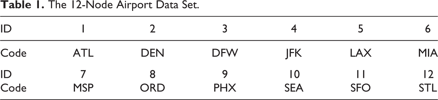
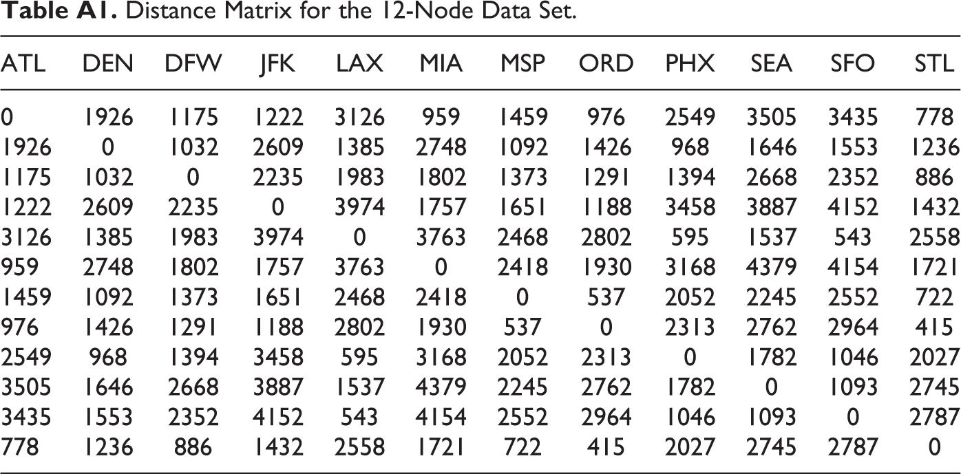
The ILP formulations of VAOMP_A, VAOMP_H, VAOMP_H2, and VAOMP_C were implemented using IBM ILOG OPL 6.3 and solved using IBM ILOG CPLEX 12.2 on a machine with dual 2.4 GHz Xeon CPUs with 24 Gigabytes of memory. The formulations were tested on three different data sets. The first one is a 12-node data set of large airports in the United States based on Lei (2010). Their standard airport codes are shown in Table 1. Distances between airports (as shown in Table A1) were calculated from the latitude and longitude using great circle arc distance and expressed in kilometers. This first data set is of a size that is comparable to that used in previous work testing OMP formulations. The second data set is the Swain (1971) 55-node data set widely used in the location science literature. A third data set of 100 US Cities (Daskin 1995) is also used to test the VAOMP_C formulation. During the computation, the parallel mode for the CPLEX engine was disabled in order to make comparisons, without including possible impacts of the parallel code. In most of the experiments, a 3-hr time limit was imposed, and if a model was not solved to optimality within this limit, we report the resulting optimality gap.
The 12-Node Airport Data Set.
Among the many possible combinations of parameter settings, we tested eighteen combinations as shown in Table 2. The first column shows the name of the problem specification. The second and third column shows the assignment vector θ and the rank vector λ, respectively. For all problems, we restricted the number of assignment levels to at most two. The last column indicates the equivalent special case problems if applicable, as discussed earlier. In the experiment, we have mainly focused on the hybrid center-median problems (which the OMP is first shown to generalize) as well as their multi-assignment extensions that are possible using the new VAOMP framework.
Tested Problem Data for the VAOMP Problem.
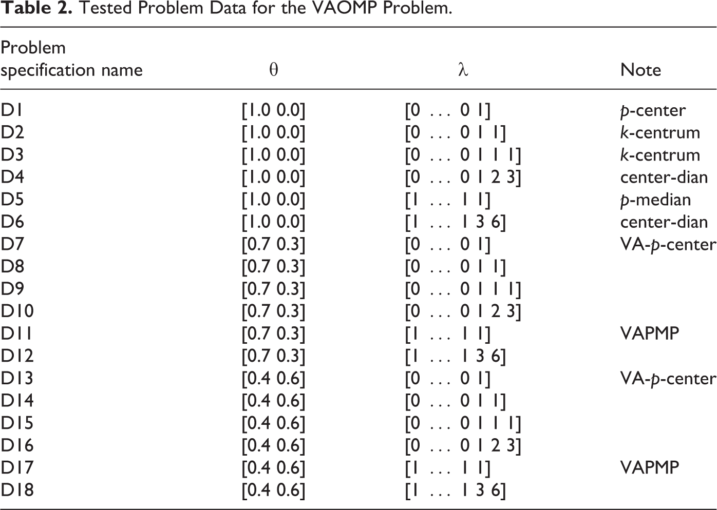
Table 3 presents computational results for the VAOMP_H formulation applied to the 12-node problem for the different problem specifications (i.e., assignment vectors θ and service rank vectors λ) specified in Table 2. In the table, the best objective values, the computation time (in seconds), the solution site patterns and optimality gap are shown in columns 2, 3, 6 and 7, respectively. Columns 4 and 5 show the number of iterations and the number of nodes expanded as reported by the CPLEX solver. The number of facilities being located was fixed at p = 5. We tested three different assignment vectors of [1 0] (D1 through D6), [0.7 0.3] (D7 through D12), and [0.4 0.6] (D13 through D18). The assignment vector [1 0] represents single-level assignment models; [0.7 0.3] can represent a reliability location problem and [0.4 0.6] represents models with assignment vectors that are not non-increasing. Six different rank vectors (λ) were tested.
VAOMP_H Results for VAOMP_H on the 12-Node Data Set (p = 5).
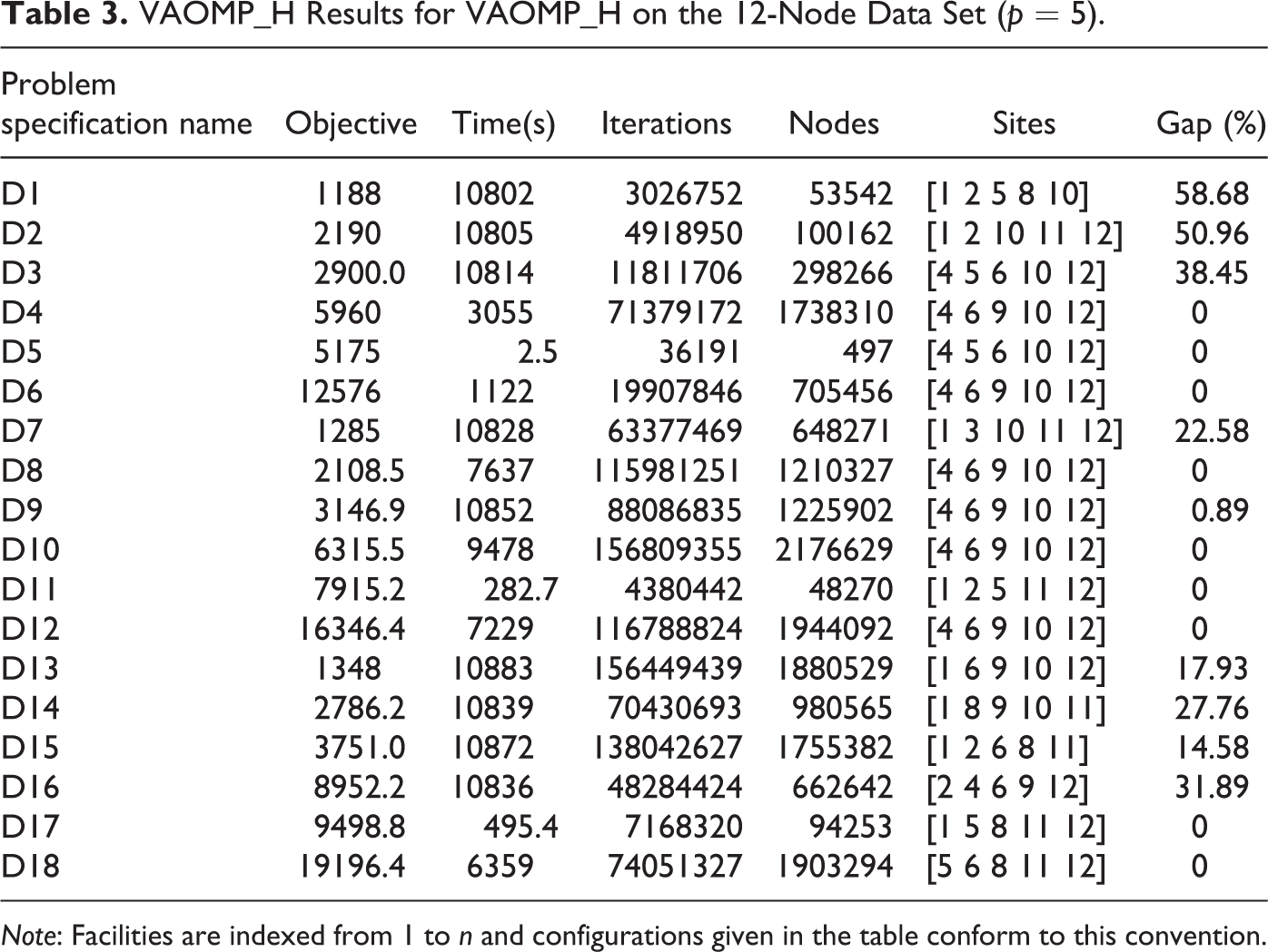
Note: Facilities are indexed from 1 to n and configurations given in the table conform to this convention.
First, we compare the objective values. For the problems with the same assignment vector, we can observe that the objective values increase when the number of nonzero entries in the rank vector λ increases. However, the average service level for each demand, which is measured by the objective value divided by the number of 1 entries in λ, decreases with an increasing number of 1 entries in λ. For example, when θ = [1 0], the average service rank for the rank vectors in D1, D2, D3, and D5 is 1188, 1095, 966.7, and 431.25, respectively. This is in accordance with the fact that this sequence of λ vectors correspond to a transition from a worst case analysis to an average case one. Similar trends can be observed for θ = [0.7 0.3] (D6 through D12) and θ = [0.4 0.6] (D13 through D18). Next, if we fix a rank vector λ, we can observe (e.g., by comparing D1, D7, and D13) that the objective values increase when the assignment vector has increasingly greater values on the second component. This can be explained by the fact that heavier weights on higher order components of an assignment vector incur greater assignment distances.
Second, we make some observations on computational time. From the third column, we can see that the computational times for all but three problem instances are very long. The three instances with short computational times are the ones that are equivalent to VAPMP instances. All other problem instances with complicated rank vectors take thousands of seconds to solve even for this 12-node data set, and more than half of the instances cannot be solved to optimality within the given time limit. This is indicative of the complexity associated with the minimax structure (and in this case, a mixed/vector assignment minimax structure).
We have also tested the VAOMP_A formulation, but they result in much longer solution times (often one magnitude longer than the corresponding VAOMP_H formulation). The longer computational times of the assignment formulation may be attributed to the large number of assignment variables. While the VAOMP_H formulation has O(Ln2) assignment variables, the VAOMP_A formulation has O(Ln3) of them.
To assess the impact of the multilevel CA constraints on the complexity of the formulation, we also tested a version VAOMP_H formulation in which the MLCA constraints are dropped. The results are shown in Table 4. Comparing Table 4 with Table 3, we can see that there is some improvement in computational times, for example, for the median type problems D5, D11, and D17. The optimality gap for those problem instances that did not solve to optimally also tends to be smaller. Another interesting observation is that for the θ = [0.4 0.6] (i.e., D17 and D18), the VAOMP_H formulation produces incorrect optimal objective values when the MLCA constraints are dropped. The optimal objective becomes lower than the true optimal. This shows the necessity of MLCA constraints whenever the assignment vector is not non-increasing.
VAOMP_H (Without Closest Assignment) on the 12-Node Data Set (p = 5).
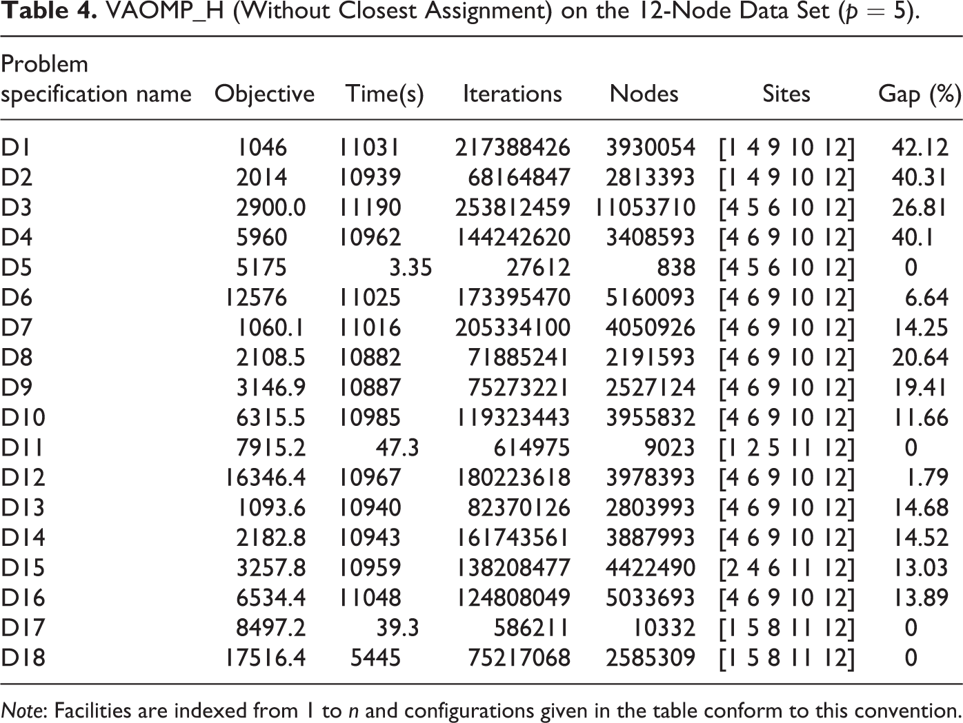
Note: Facilities are indexed from 1 to n and configurations given in the table conform to this convention.
Table 5 presents computational results for the VAOMP_H2 formulation. From this table, we can observe that the VAOMP_H2 formulation is significantly slower than VAOMP_H. For one instance (D12), no feasible solution was found within 3 hr. With few exceptions, the VAOMP_H2 formulation either involves longer solution times or larger optimality gaps than the VAOMP_H formulation.
VAOMP_H2 Results on the 12-Node Data Set (p = 5).
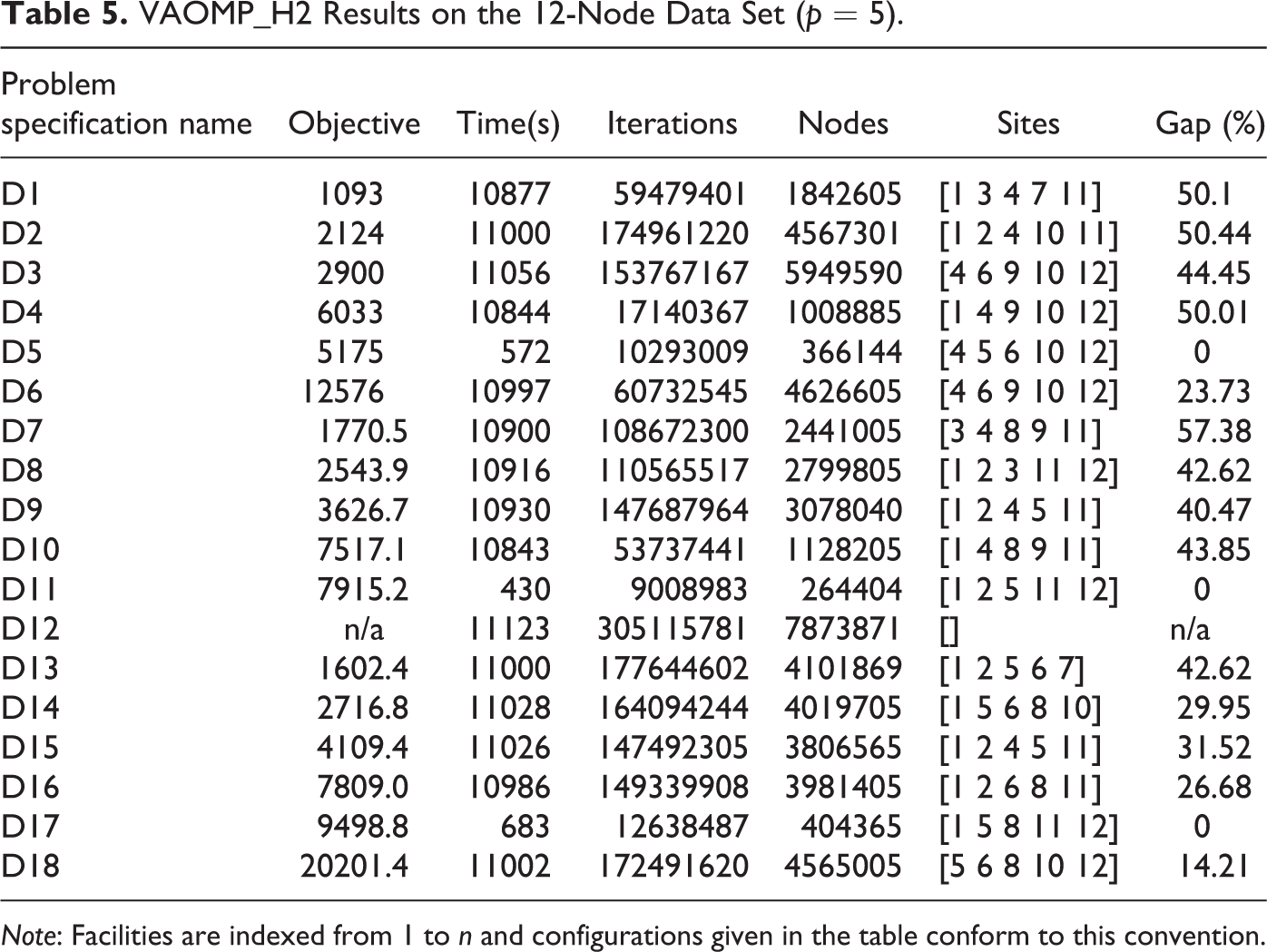
Note: Facilities are indexed from 1 to n and configurations given in the table conform to this convention.
Overall, the computational experiments in this section show that the VAOMP problem has a very high complexity. Among the general formulations tested above, VAOMP_H outperforms the other two formulations. Next, we test the special-case formulation VAOMP_C, which is suitable for problem instances with non-decreasing rank vectors. It should be noted, however, that this special-case model covers the “distance minimizing” problems involving a combination of worst case and average case analysis, which probably represents what is more commonly used in location problems.
Table 6 presents computational results for running the VAOMP_C results on the 12-node data set. Comparing this table with Tables 3 and 4, we can see a significant improvement in computation times. All problem instances are solved to optimality within less than a second. Except for the “median” problem instances D5, the solution times for the VAOMP_C formulation are at least three orders of magnitudes lower than that of the VAOMP_H and VAOMP_H2 formulations. This is in accordance with findings in prior work (see e.g., Nickel and Puerto 2005) that such problems are easier to solve than the general OMP. The improved efficiency of the VAOMP_C formulation is also evident from the significantly lower numbers of iterations and expanded nodes.
VAOMP_C Results on the 12-Node Data Set (p = 5).
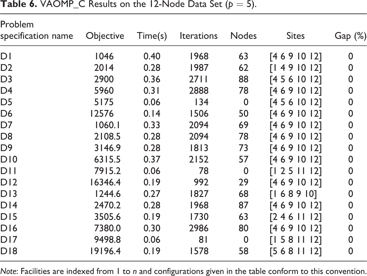
Note: Facilities are indexed from 1 to n and configurations given in the table conform to this convention.
We also tested the VAOMP_C formulation on the (unweighted) Swain 55 node data set which is widely used in location science for testing median, center, and other problems, and the results are presented in Table 7. We can see from this table that even for this medium sized data set, all problem instances from D1 through D18 can be solved to optimality within less than 45 min. Most instances can be solved in less than 15 min, with the exception of the center-type or center-like problems (D1, D2, and D7).
VAOMP_C Results on the Swain 55-node Data Set (p = 5).
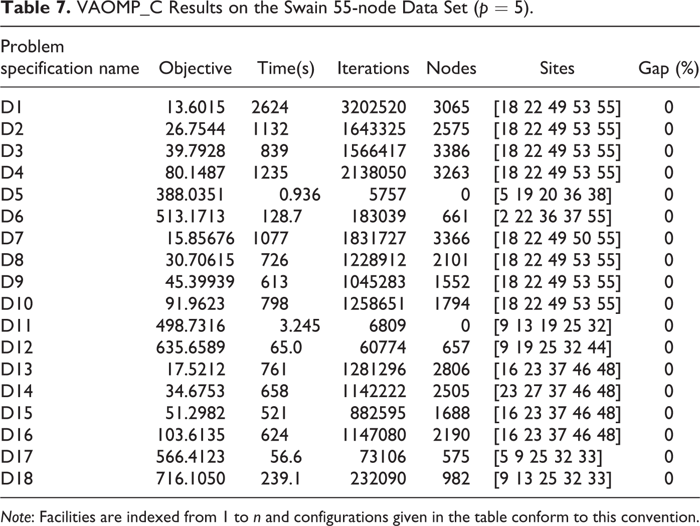
Note: Facilities are indexed from 1 to n and configurations given in the table conform to this convention.
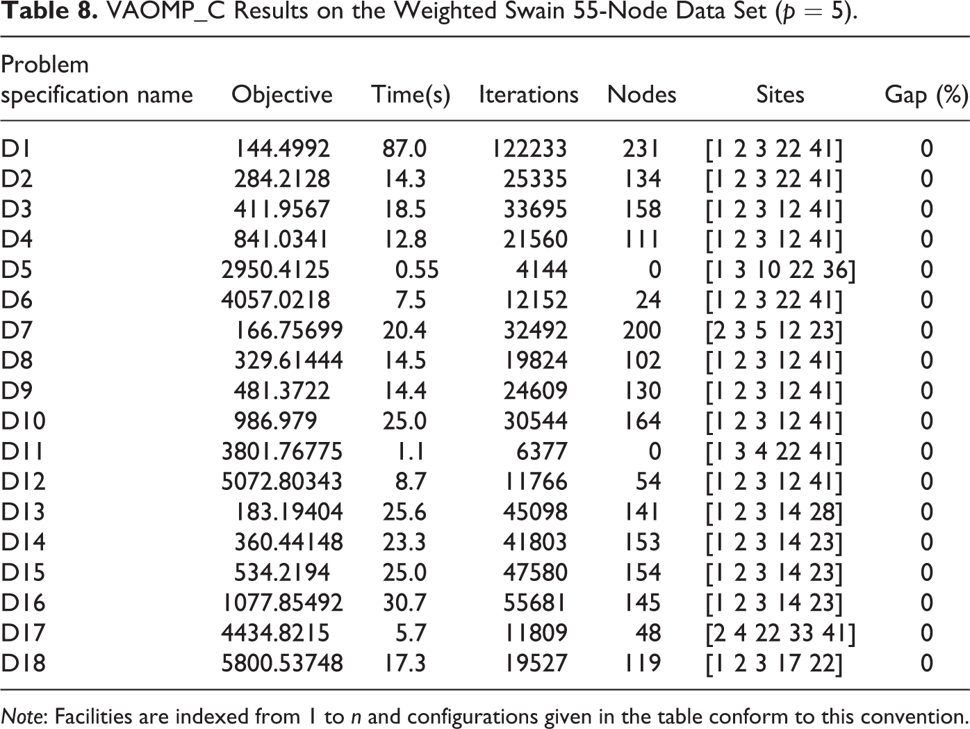
Since the p-median problem and many other location problems are often posed with population on the demands, we also tested the VAOMP_C formulation on the original Swain data set with the weight data in order to facilitate comparison with known results in the literature. The VAOMP_C results are presented in Table 8. We can see from this table that (at least for this data set) the computational times for the weighted problem are significantly less (by about one or two orders of magnitudes) than the unweighted case.
VAOMP_C Results on the Weighted Swain 55-Node Data Set (p = 5).
Note: Facilities are indexed from 1 to n and configurations given in the table conform to this convention.
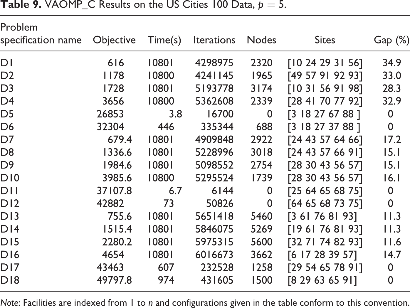
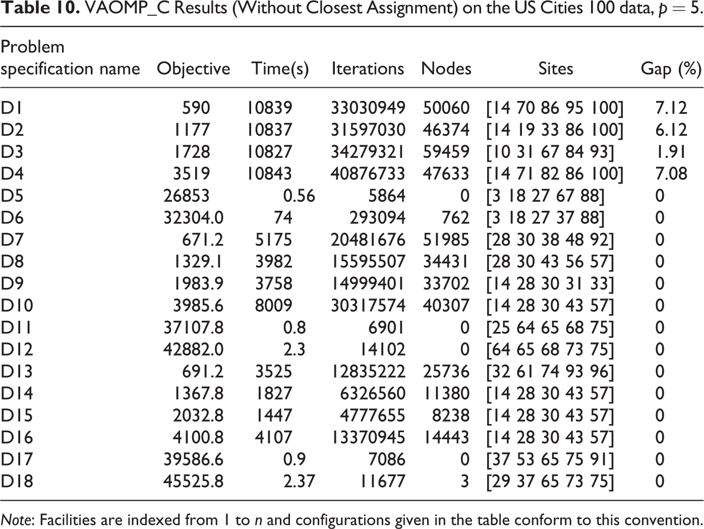
We also used a larger US Cities 100 data set, which contains the first 100 cities from the US Cities data set in Daskin (1995), to test the performance of the VAOMP_C formulation. Weights on demands were again not used. The computational results are presented in Table 9. We can observe that the Vector Assignment-PMP and “center-dian” problems, namely, D5, D6, D11, D12, D17, and D18, can be solved optimally, with solution times ranging from a few seconds to 15 min. All other problem instances (i.e., the VA-center and k-centrum problems) could not be solved optimally within the 3-hr time limit. The optimality gaps ranged from 11 percent to 35 percent. As observed earlier, the CA constraints can be dropped when the assignment vector is non-increasing. Table 10 presents computational results for solving a variant of the VAOMP_C formulation which did not include CA constraints. We can observe that dropping CA constraints significantly improved the performance of the formulation. While only six of the eighteen problems in Table 9 could be solved optimally, fourteen of the eighteen problems in Table 10 could be solved. The maximum optimality gap was reduced from 35 percent to about 7 percent. Again, it is important to note that for problems D13 through D18, dropping CA conditions leads to incorrect solutions as the assignment vector is not non-increasing.
VAOMP_C Results on the US Cities 100 Data, p = 5.
Note: Facilities are indexed from 1 to n and configurations given in the table conform to this convention.
VAOMP_C Results (Without Closest Assignment) on the US Cities 100 data, p = 5.
Note: Facilities are indexed from 1 to n and configurations given in the table conform to this convention.
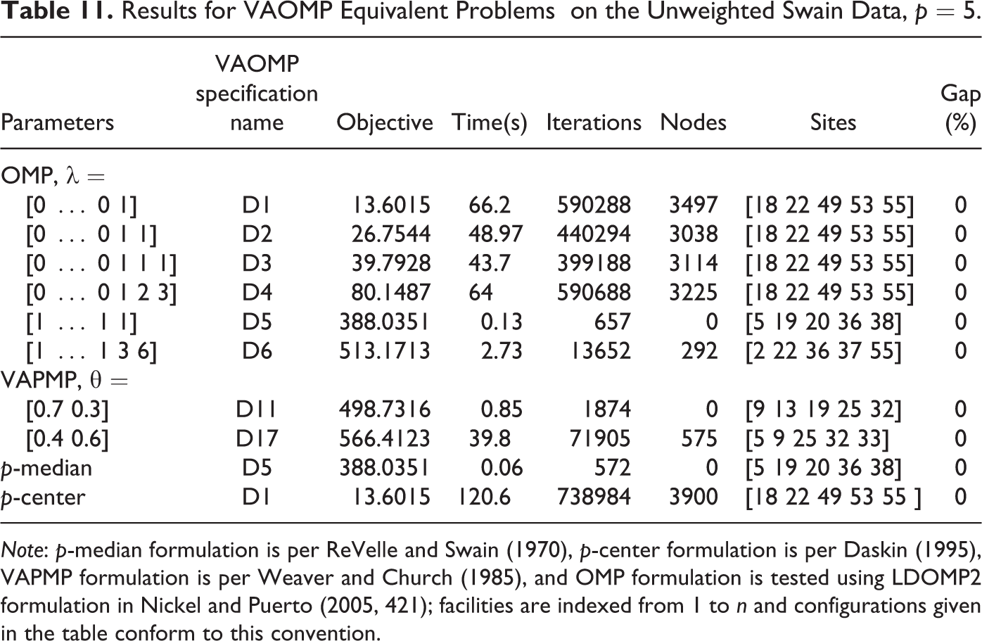
Finally, we compare the performances of the VAOMP model to those of the formulations specifically designed to solve the special cases problems noted in Table 2, namely, the OMP, the VAPMP, and p-median problem and the p-center problem. The OMP is implemented according to an OMP formulation in Nickel and Puerto (2005, 421). The VAPMP formulation is implemented according to Weaver and Church (1985) except that MLCA constraints in Lei and Church (2011a) were added. The p-median problem and the p-center problems were implemented according to the formulations in ReVelle and Swain (1970) and Daskin (1995) respectively. Table 11 presents results for solving the special case problems on the unweighted Swain data set. Problem specific parameters and the corresponding VAOMP specification names were listed in columns 1 and 2, respectively.
Results for VAOMP Equivalent Problems on the Unweighted Swain Data, p = 5.
Note: p-median formulation is per ReVelle and Swain (1970), p-center formulation is per Daskin (1995), VAPMP formulation is per Weaver and Church (1985), and OMP formulation is tested using LDOMP2 formulation in Nickel and Puerto (2005, 421); facilities are indexed from 1 to n and configurations given in the table conform to this convention.
Comparing Table 11 with Table 7, we can observe that the formulations specifically designed for the special-case problems are faster than VAOMP_C. The OMP formulation is 8 to 50 times faster than VAOMP_C. The VAPMP formulation was slightly faster than VAOMP_C in solving equivalent problems. While it took VAOMP_C 3.2 and 57 s to solve D11 and D17 problems, the VAPMP formulation took only 0.9 and 40 s, respectively. This shows that the overhead of VAOMP_C over VAPMP is not large. By comparison, the p-median formulation is 10 times and 50 times faster than the VAPMP and VAOMP_C formulations, respectively. The p-center formulation is about 20 times faster than VAOMP_C. Table 12 shows a similar comparison of VAOMP_C and special case formulations for the weighted Swain data set. The OMP formulation is 5 to 50 times faster than VAOMP_C. The p-median formulation is about 10 times faster and the VAPMP formulation is slightly faster than VAOMP_C. This difference is hardly surprising because all tested special-case problems except the VAPMP requires CA constraints.
To summarize the computational experiments in this section, we can see that the VAOMP problem is a very difficult problem to solve in general. General formulations such as VAOMP_H involve long solution times even for a very small 12-node data set. On the other hand, the VAOMP_C formulation is suitable for a special-case (yet also very general) VAOMP problem, confirming prior results (see e.g., Nickel and Puerto 2005) about the effectiveness of similar formulations for the OMP. It can be solved within short computation times even for a median sized problem. The computation times for different special cases of VAOMP vary. In general, our results show that the center-type or center-like problems are clearly harder to solve, as what has been experienced in the literature.
Results for VAOMP Equivalent Problems on the Weighted Swain Data, p = 5.
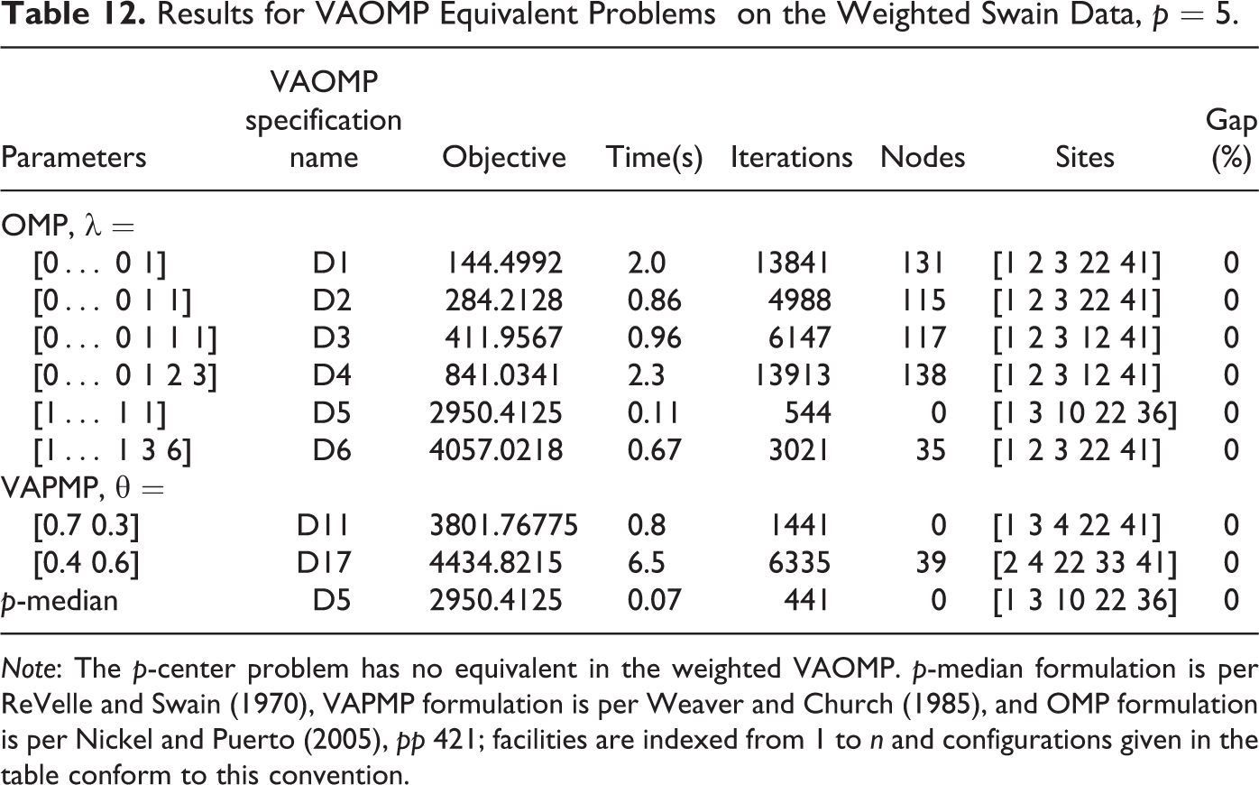
Note: The p-center problem has no equivalent in the weighted VAOMP. p-median formulation is per ReVelle and Swain (1970), VAPMP formulation is per Weaver and Church (1985), and OMP formulation is per Nickel and Puerto (2005), pp 421; facilities are indexed from 1 to n and configurations given in the table conform to this convention.
Conclusions
Past research work has proposed several generalized constructs; among these are the OMP and the VAPMP. In this article, we have proposed a general problem that subsumes both constructs into one general framework, called VAOMP (vector assignment ordered median problem). In this article, we have presented several formulations for VAOMP. These new models are sensitive to distance and integrate explicit constraints which can enforce CA under various special case conditions of the general problem. We have shown that VAOMP is a very general model structure that can subsume as special cases a large number of location-allocation problems including ordered median, reliability location problems, multilevel covering, fault-tolerant location, and interdiction.
The ILP formulations developed in this article can be solved directly by off-the-shelf solvers. We have also analyzed the VAOMP and identified the conditions under which certain constraint structures can be omitted from the formulation.
We tested four different formulations of the VAOMP problem. Our experiments show that it takes a significant amount of computation time in finding optimal solutions for the general form of the problem. However, in the special case where the rank vector λ is non-decreasing and non-negative, the VAOMP_C formulation can solve almost all the tested problem instances in a relatively short amount of time, even for a medium-sized problem. A number of research directions involving VAOMP are possible and may be quite fruitful. This includes, for example, the development of effective heuristic or approximate algorithms for the general VAOMP, the design of branch and bound algorithms, and using externally derived bounds to tighten the VAOMP formulations by fixing variables and adding valid inequalities.
Footnotes
Appendix A
Distance Matrix for the 12-Node Data Set.
| ATL | DEN | DFW | JFK | LAX | MIA | MSP | ORD | PHX | SEA | SFO | STL |
|---|---|---|---|---|---|---|---|---|---|---|---|
| 0 | 1926 | 1175 | 1222 | 3126 | 959 | 1459 | 976 | 2549 | 3505 | 3435 | 778 |
| 1926 | 0 | 1032 | 2609 | 1385 | 2748 | 1092 | 1426 | 968 | 1646 | 1553 | 1236 |
| 1175 | 1032 | 0 | 2235 | 1983 | 1802 | 1373 | 1291 | 1394 | 2668 | 2352 | 886 |
| 1222 | 2609 | 2235 | 0 | 3974 | 1757 | 1651 | 1188 | 3458 | 3887 | 4152 | 1432 |
| 3126 | 1385 | 1983 | 3974 | 0 | 3763 | 2468 | 2802 | 595 | 1537 | 543 | 2558 |
| 959 | 2748 | 1802 | 1757 | 3763 | 0 | 2418 | 1930 | 3168 | 4379 | 4154 | 1721 |
| 1459 | 1092 | 1373 | 1651 | 2468 | 2418 | 0 | 537 | 2052 | 2245 | 2552 | 722 |
| 976 | 1426 | 1291 | 1188 | 2802 | 1930 | 537 | 0 | 2313 | 2762 | 2964 | 415 |
| 2549 | 968 | 1394 | 3458 | 595 | 3168 | 2052 | 2313 | 0 | 1782 | 1046 | 2027 |
| 3505 | 1646 | 2668 | 3887 | 1537 | 4379 | 2245 | 2762 | 1782 | 0 | 1093 | 2745 |
| 3435 | 1553 | 2352 | 4152 | 543 | 4154 | 2552 | 2964 | 1046 | 1093 | 0 | 2787 |
| 778 | 1236 | 886 | 1432 | 2558 | 1721 | 722 | 415 | 2027 | 2745 | 2787 | 0 |
Declaration of Conflicting Interests
The author(s) declared no potential conflicts of interest with respect to the research, authorship, and/or publication of this article.
Funding
The author(s) received no financial support for the research, authorship, and/or publication of this article.